Power law correlations in galaxy distribution and finite volume effects from the Sloan Digital Sky Survey Data Release Four

We discuss the estimation of galaxy correlation properties in several volume limited samples, in different sky regions, obtained from the Fourth Data Release of the Sloan Digital Sky Survey. The small scale properties are characterized through the determination of the nearest neighbor probability distribution. By using a very conservative statistical analysis, in the range of scales [0.5,$\sim$ 30] Mpc/h we detect power-law correlations in the conditional density in redshift space, with an exponent $\gamma=1.0\pm 0.1$. This behavior is stable in all different samples we considered thus it does not depend on galaxy luminosity. In the range of scales [$\sim$ 30,$\sim$ 100] Mpc/h we find evidences for systematic unaveraged fluctuations and we discuss in detail the problems induced by finite volume effects on the determination of the conditional density. We conclude that in such range of scales there is an evidence for a smaller power-law index of the conditional density. However we cannot distinguish between two possibilities: (i) that a crossover to homogeneity (corresponding to $\gamma=0$ in the conditional density) occurs before 100 Mpc/h, (ii) that correlations extend to scales of order 100 Mpc/h (with a smaller exponent $0<\gamma<1$). We emphasize that galaxy distributions in these samples present large fluctuations at the largest scales probed, corresponding to the presence of large scale structures extending up to the boundaries of the present survey. Finally we discuss several differences between the behavior of the conditional density in mock galaxy catalogs built from cosmological N-body simulations and real data. We discuss some theoretical implications of such a fact considering also the super-homogeneous features of primordial density fields.

1 Introduction

One of the main open problems in modern cosmology is represented by the statistical characterization and the physical understanding of large scale galaxy structures. The first question in this context concerns the studies of galaxy correlation properties. Particularly two-point properties are useful to determine correlations and their spatial extension. There are different ways of measuring two-point properties and, in general, the most suitable method depends on the type of correlations, strong or weak, characterizing a given point distribution in a certain sample.

For example, Hogg et al. (2005) have recently measured the conditional average density in a sample of Luminous Red Galaxies (LRG) from a data release of the Sloan Digital Sky Survey (SDSS). Such a statistics is very useful to determine correlation properties in the regime of strong clustering and the spatial extension of strong fluctuations in a given sample. This was firstly introduced by Pietronero (1987) and then measured in many samples by Sylos Labini et al. (1998). We refer the reader to Baryshev & Teerikorpi (2005) for a review of the measurements of the reduced and complete correlation functions by different authors in the various angular and three-dimensional samples.

The conditional density gives the average density of points in a spherical volume (or a spherical shell) centered around a galaxy (see Gabrielli et al. 2004 for a discussion about this method). The results obtained by Hogg et al. (2005) can be summarized as follows:

(i) A simple power-law scaling corresponding to a correlation exponent $\gamma\approx 1$ gives a very good fit to the data up to at least $20$ Mpc/h, over approximately a decade in scale. We note that these results are in good agreement with those obtained by Sylos Labini et al. (1998) through the analyses of many smaller samples and more recently by Vasilyev, Baryshev and Sylos Labini (2006) in the 2dFGRS.

(ii) The second important result of Hogg et al. (2005) is that at larger scales (i.e. $r>30$ Mpc/h) the conditional density continues to decrease, but less rapidly, until about $\sim 70$ Mpc/h, above which it seems to flatten up to the largest scale probed by the sample ($100$ Mpc/h). The transition between the two regimes is slow, in the sense that the conditional density at $\sim 20$ Mpc/h is about twice the asymptotic mean density. Joyce et al. (2005) have discussed the basic implications of these results noticing, for example, that the possible convergence to a well defined homogeneity in a volume equivalent to that of a sphere of radius 70 Mpc/h, place in doubt previous detections of “luminosity bias” from measures of the amplitude of the reduced correlation function $\xi(r)$. They emphasized that the way to resolve these issues is to first use, in volume limited (VL) samples corresponding to different ranges of luminosity, the conditional density to establish the features of galaxy space correlations. Note that Sylos Labini et al. (1998) found evidences for a continuation of the small scale power-law to distances of order hundreds of Mpc/h, although with a weaker statistics, which seems to be not confirmed by Hogg et al. (2005).

In this paper we continue the analysis of galaxy distributions previously applied to the 2dFGRS data (Vasilyev et al. 2006) to the so-called “main galaxy sample” of SDSS Data Release (DR4), in the spirit of the tests discussed above. In a companion paper we will discuss the properties of the LRG sample of the SDSS DR4, which can be directly compared with the results of Hogg et al. (2005) and Eiseinstein et al. (2005).

The paper is organized as follows. In Section 2 we describe the data and the way we have constructed the VL samples. We also discuss the determination of the nearest neighbor (NN) distribution, and of the average distance between nearest galaxies, which allows us to define the lower cut-off for the studies of correlations. In addition we discuss the determination of the radial counts in different VL samples, emphasizing that large variations for this quantity are found in the different samples. Such fluctuations, which seem to be persistent up to the sample boundaries, correspond to the large scales structures observed in these catalogs. The quantitative characterization of the correlation properties of these fluctuations is presented in Section 3, where we discuss the determination of the conditional average density in the different VL samples. In particular we present several tests useful to clarify the effect of systematic fluctuations at scales of order of the samples size.

In Section 4 we discuss the differences between the galaxy conditional density, measured in these samples and the conditional density of point-particles in cosmological N-body simulations. We show that by using this statistics, together with a study of the NN probability distribution, two-point properties of observed galaxies of different luminosity and mock galaxy catalogs constructed using particles lying in region with different local density in cosmological N-body simulations, present different behaviors. Finally in Section 5 we draw our main conclusions.

2 The data

The SDSS (http://www.sdss.org) is currently the largest spectroscopic survey of the extragalactic objects and one of the most ambitious observational programs ever undertaken in astronomy. It will measure about 1 million redshifts, giving a complete mapping of the local universe up to a depth of several hundreds of Mpc. In this paper we consider the data from the latest public data release (SDSS DR4) which is accessible at http://www.sdss.org/dr4 (Adelman-McCarthy et al. 2005) containing redshifts for more than 565 thousands of galaxies and 67 thousands of quasars. There are two independent parts of the galaxy survey in the SDSS: the main galaxy sample and the LRG sample. Here we discuss the former only. The spectroscopic survey covers an area of 4783 square degrees of the celestial sphere. The apparent magnitude limit for the galaxies is 17.77 in the $r$-filter and photometry for each galaxy is available in five different bands, of which we consider the ones in the $r$ and $g$ filters.

2.1 Definition of the samples

We have used the following criteria to query the SDSS DR4 database. First of all we constrain the flags indicating the type of object so that we select only the objects from the main galaxy sample. We then consider galaxies in the redshift interval $10^{-4}\leq z\leq 0.3$ and with the redshift confidence parameter larger than $0.95$. In addition we apply the filtering condition $r<17.77$, thus taking into account the target magnitude limit for the main galaxy sample in the SDSS DR4. With the respect to the listed conditions we have selected 321516 objects totally.

The angular coverage of the survey is not uniform but observations have been done in different sky regions. For this reason we have considered three rectangular angular fields (named R1, R2 and R3) in the SDSS internal angular coordinates $(\eta,\lambda)$: in such a way we do not have to consider the irregular boundaries of the survey mask, as we have cut such boundaries to avoid uneven edges of observed regions. In Tab.1 we report the parameters of the three angular regions we have considered. In addition we do not use corrections neither for the redshift completeness mask nor for the fiber collision effects. Completeness varies mostly nearby the current survey edges which are excluded in our samples. Fiber collisions in general do not represent a problem for measurements of galaxy correlations (see discussion in, e.g., Strauss et al., 2002).

Region name	$\eta_{1}$	$\eta_{2}$	$\lambda_{1}$	$\lambda_{2}$	$\Omega$
R1	9.0	36.0	-47.0	8.0	0.41
R2	-33.5	-16.5	-54.0	-24.0	0.12
R3	-36.0	-26.5	2.5	43.0	0.11

Table 1: Main properties of the angular regions considered: The limits in degrees of the cuts are chosen using the intrinsic coordinates of the survey $\eta$ and $\lambda$ (in degrees). The last column $\Omega$ gives the solid angle of three angular regions in steradians.

2.2 Construction of VL samples

To construct VL samples which are unbiased for the selection effect related to the cut in the apparent magnitude, we have applied a standard procedure (see e.g. Zehavi et al., 2004): First of all we compute metric distances as

$$r(z)=\frac{c}{H_{0}}\int_{\frac{1}{1+z}}^{1}{\frac{dy}{y\cdot\left(\Omega_{M}/y+\Omega_{\Lambda}\cdot y^{2}\right)^{1/2}}}\;,$$ (1)

where we have used the standard cosmological parameters $\Omega_{M}=0.3$ and $\Omega_{\Lambda}=0.7$ with $H_{0}=100h$ km/sec/Mpc.

We use Petrosian apparent magnitudes in the $r$ filter $m_{r}$ which are corrected for galactic absorption. The absolute magnitudes can be computed as

$$M_{r}=m_{r}-5\cdot\log_{10}\left[r(z)\cdot(1+z)\right]-K_{r}(z)-25.$$ (2)

where $K_{r}(z)$ is the K-correction. As the redshift range considered is small from a cosmological point of view (i.e. $z\leq 0.3$), to estimate the K-corrections $K_{r}(z)$ (linearly proportional to $z$ and thus small in this context) we have used the simple interpolating formula

$$K_{r}(z)=(2.61\cdot(m_{g}-m_{r})-0.64)\cdot z\;,$$ (3)

where $m_{g}$ is the apparent magnitude in the $g$ filter. This corresponds to the calculated K-corrections in Blanton et al. (2001 — see their Fig.4). By knowing the intrinsic $g-r$ color and the redshift one may directly estimate the K-correction term.

We have considered 4 different VL samples (named VL1, VL2, VL3 and VL4) defined by two chosen limits in absolute magnitude and metric distance, whose parameters are reported in Tab.2. While VL1 and VL2 actually contain relatively faint galaxies in the local universe, VL3 sample covers a wide range of distances, and VL4 consists of bright galaxies at distances up to 600 Mpc/h. Considering the three different rectangular areas (described above), in summary we have $4\times 3=12$ VL subsamples whose characteristics are reported in Tab.3. The comparison between VL samples with the same magnitude and distance cuts, in different sky regions, will allow us to test the statistical stationarity of galaxy distributions in these samples and to estimate sample-to-sample fluctuations.

VL sample	$r_{min}$	$r_{max}$	$M_{min}$	$M_{max}$	$\langle\Lambda\rangle$
VL1	50	135	-19.0	-18.0	1.7
VL2	50	200	-21.0	-19.0	1.3
VL3	100	500	-23.0	-21.0	2.9
VL4	150	600	-23.0	-22.0	6

Table 2: Main properties of the obtained VL samples: $r_{min}$, $r_{max}$ (in Mpc/h) are the chosen limits for the metric distance; ${M_{min},\,M_{max}}$ define the interval for the absolute magnitude in each sample. The quantity $\langle\Lambda\rangle$ (in Mpc/h) is the average distance between nearest-neighbor galaxies.

VL Sample	N	$R_{c}$
R1VL1	3130	15
R1VL2	15181	21
R1VL3	27975	54
R1VL4	6742	65
R2VL1	790	10
R2VL2	3912	15
R2VL3	8586	38
R2VL4	1923	42
R3VL1	790	9
R3VL2	2895	12
R3VL3	7584	30
R3VL4	1503	36

Table 3: Number of galaxies in each of the VL sample. Names are given according to the discussion in the text. The scale $R_{c}$ (in Mpc/h) is discussed in Sect.3.2 below.

2.3 Nearest neighbor distribution

The NN distance probability distribution depends on the cut in absolute magnitude of a given VL sample. We expect this function not to be dependent on the angular sky cuts if the distribution is statistically stationary in the different VL samples. As discussed in Vasilyev, Baryshev & Sylos Labini (2006) space correlations introduce a deviation from the case of a pure Poisson distribution: particularly the average distance $\langle\Lambda\rangle$ between NN is expected to be smaller than for the Poisson case in the same sample and with the same number of points. The measurements in the data, obtained by simple pair-counting, are shown in Figs.1-4. When a VL sample includes fainter galaxies (e.g. VL1,VL2) $\langle\Lambda\rangle$ is smaller (see Tab.2) than for the case when only brighter galaxies are inside (e.g. VL3,VL4). This is because brighter galaxies are sparser than fainter ones. This corresponds to the exponential decay of the galaxy luminosity function at the bright end (see discussion in Gabrielli et al., 2004)

Figure 1: Nearest Neighbor distribution in VL1 sample: different symbols correspond to different angular regions. The average distance between nearest galaxies is $\langle\Lambda\rangle=1.7$ Mpc/h. For reference the solid line represents the NN distribution for a Poisson configuration with the same $\langle\Lambda\rangle$: one may notice that the tails of this function decay more rapidly.

Figure 2: As Fig.1 but for the VL2 samples. The average distance between galaxies is $\langle\Lambda\rangle=1.3$ Mpc/h.

Figure 3: As Fig.1 but for the VL3 samples. The average distance between nearest galaxies is $\langle\Lambda\rangle=2.9$ Mpc/h.

Figure 4: As Fig.1 but for the VL4 samples.The average distance between nearest galaxies is $\langle\Lambda\rangle=6$ Mpc/h.

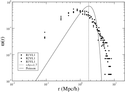
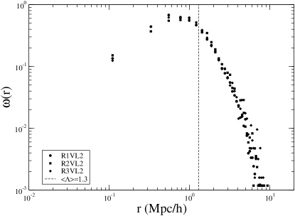
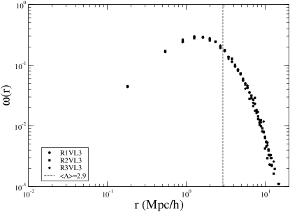
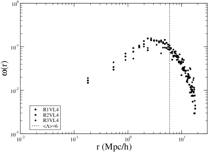
Note that Zehavi et al. (2004) have estimated that at scale of order $1\div 2$ Mpc/h there is a departure from a power law behavior in the reduced correlation function. At the light of the discussion above we stress that this change occurs in a range of scales where NN correlations are dominant in all samples considered. For the interpretation of this behavior one may consider the relation between the conditional density, or the reduced correlation function, and the NN probability distribution (see Baertschiger & Sylos Labini 2004 for a discussion of this point). In this respect, in the comparison of galaxy data with N-body simulations, one has to be careful in that these small-scale properties can be determined by sampling, sparseness and other more subtle finite size effects related to the precision of a given N-body simulation (Baertschiger & Sylos Labini 2004).

We have then studied the effect of the fiber collisions on the NN statistic: about $6\%$ of galaxies that satisfy the selection criteria of the main galaxy sample are not observed because they have a companion closer than the 55 arc-sec minimum separation of spectroscopic fibers (Strauss et al., 2002). However not all 55-arc-sec pairs are affected by fiber collisions, because some of the SDSS were observed spectroscopically more than once. We have identified all $<=55$ arc-sec pairs for which both galaxies have redshifts, and we have randomly removed one of those redshifts in each case to make a new sample with an even more severe fiber collision problem than the existing sample. Because of the very small number of galaxy pairs with angular separation $<=55$ arc-sec (of order of few percent in all the volume limited samples we have considered) there is no sensible effect of the results. In fact, for galaxies in the main sample the average redshift $z\sim 0.1$, and hence the angular distance 55 arc-sec corresponds to the linear separation $r\sim 0.1$ Mpc/h which is marginally outside the scales interval we have studied the NN distribution, i.e. $r>0.2$ Mpc/h. Hence we expect that the fiber collision effect does not influence our results as indeed we find.

2.4 Number counts in VL samples

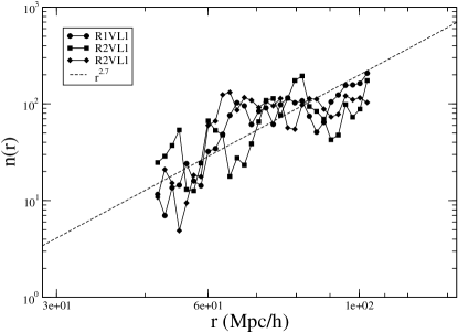
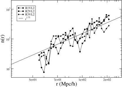
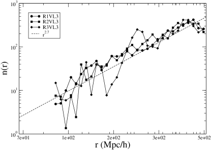
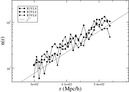
A simple statistics which can be easily computed in VL samples is represented by the differential number counts. This gives us a first indication about (i) the slope of the counts and (ii) the nature of fluctuations (see e.g. Gabrielli et al. 2004). In general we may write that the number of points counted from a given point chosen as origin (in this case the Earth) grows as

$$N(r)\sim r^{D}\;.$$ (4)

This represents the radial counts in a spherical volume of radius $r$ around the observer (or in a portion of a sphere). In the case $D=3$ the distribution is uniform and $D<3$ if it is, for example, fractal or if there is a systematic effect of depletion of points as a function of distance. In this situation we neglect relativistic effects, which are anyway small in the range of redshift considered. However as noticed by Gabrielli et al. (2004) these corrections may change the slope of the counts but not the intrinsic fluctuations.

Given that a VL sample is defined by two cuts in distance we compute

$$n(r)=\frac{dN(r)}{dr}\sim r^{D-1}\;,$$ (5)

i.e. the differential number counts in shells. Simply stated we expect the exponent in Eq.5 to be 2 when the distribution is uniform; in this case we also expect to see small (normalized) fluctuations generally decaying as the volume or faster for the case of super-homogeneous case (i.e. for standard cosmological density fields — see discussion in Gabrielli et al., 2004)

Results in the samples considered are shown in Figs.5-8, where for each sample we have normalized the counts to the solid angle of the corresponding angular region. One may note that the best fit exponent (reported in the figures) fluctuates, and in several case it is larger than 2. This means that there are large fluctuations as evidenced by the non-smooth behaviors of $n(r)$ in the different samples. A similar evidence of the effect of large scale structures in these samples on other statistical quantities has been recently pointed out by Nichol et al. (2006).

This is a first rough indication that the question of uniformity at scales of order 100 Mpc/h is not simple to be sorted out in these samples. These large fluctuations in slope and amplitude correspond to the presence of large scale galaxy structures extending up to the boundaries of the various samples considered. We do not present a more quantitative discussion of these behaviors as the statistics is rather weak.

Figure 5: Differential number counts as a function of distance in the VL1 sample in different angular regions normalized to their own solid angle

Figure 6: The same as Fig.5 but for the VL2 samples

Figure 7: The same as Fig.5 but for the VL3 samples

Figure 8: The same as Fig.5 but for the VL4 samples

3 Correlation properties of galaxy distributions

We study now the behavior of the conditional average density in the various VL samples discussed in the previous section. We use the full-shell estimator, discussed extensively in Gabrielli et al. (2004) and recently in Vasilyev, Baryshev & Sylos Labini (2006). This estimator has the advantage of making no assumption in the treatment of boundary conditions and it is the more conservative one among estimators of two-pint correlations (see discussion in Kerscher,1999). Briefly the conditional density in spheres $\langle n(r)^{*}\rangle_{p}$ is defined for an ensemble of realizations of a given point process, as

$$\langle n(r)^{*}\rangle_{p}=\frac{\langle{N(r)}\rangle_{p}}{V(r)}.$$ (6)

This quantity measures the average number of points $\langle{N(r)}\rangle_{p}$ contained in a sphere of volume $V(r)=\frac{4}{3}\pi{r}^{3}$ with the condition that the center of the sphere lies on an occupied point of the distribution (and $\langle{...}\rangle_{p}$ denotes the conditional ensemble average). Such a quantity can be estimated in a finite sample by a volume average (supposing ergodicity of the point distribution)

$$\langle n(r)^{*}\rangle_{p}=\frac{1}{N_{c}(r)}\sum_{i=1}^{N_{c}(r)}{\frac{N_{i}(r)}{V(r)}},$$ (7)

where $N_{c}(r)$ — the number of points for which, when chosen as centers of a sphere of radius $r$, this is fully contained in the sample volume — averaging by the sample points. (The estimation of the conditional density in shells $\langle n(r)\rangle_{p}$ proceeds in the same way, except for the fact of considering spherical shells instead of spheres centered on the points — see e.g. Vasilyev, Baryshev & Sylos Labini 2006).

Therefore this full-shell estimator has an important constraint: it is measured only in spherical volumes fully included in the sample volume. In this situation the number of centers $N_{c}(r)$ over which the average Eq.7 is performed, becomes strongly dependent on the scale $r$ when $r\rightarrow R_{s}$, being $R_{s}$ the sample size. In this context such a length scale can be defined as the radius of the largest sphere fully included in the sample volume: the center of such a sphere lies in the middle of the sample volume.

Thus, when approaching the scale $R_{s}$ there are two sources of fluctuations which increase the variance of the measurements. From the one hand the number of points over which the average is performed decreases very rapidly and from the other hand the remaining points are concentrated toward the center of the sample. In such a way systematic fluctuations may affect the estimation, given that these are not averaged out by the volume average. An estimation of the scale beyond which systematic effects become strong and thus important.

The following subsection is focused to the discussion of the measurements of $\langle n(r)^{*}\rangle_{p}$ in the different VL samples, while Sect.3.2 is devoted to the problem of the determination of the maximum scale up to which the volume average is properly performed, and thus beyond which systematic unaveraged fluctuations may affect the behavior of the conditional density.

3.1 Estimation of the conditional density

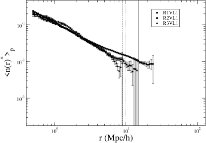
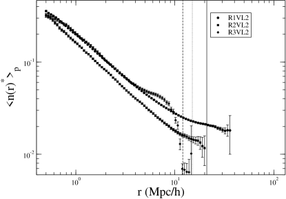
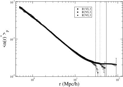
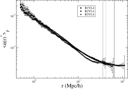
The results of the measurements in redshift space of the conditional density by the full-shell estimator, in VL samples with the same cuts in absolute magnitude and distance but in different angular regions, are reported in Figs.9-12. The formal statistical error, reported in the figures, for the determination of $\langle n(r)^{*}\rangle_{p}$ at each scale, can be simply derived from the dispersion of the average

$$\Sigma^{2}(r)=\frac{1}{N_{c}(r)}\sum_{i=1}^{N_{c}(r)-1}\frac{\left(n(r)_{i}^{*}-\langle n(r)^{*}\rangle_{p}\right)^{2}}{N_{c}(r)-1}\;,$$ (8)

where $n(r)_{i}^{*}$ represents the determination from the $i^{th}$ point. One may see that such an error is very small, except for the last few points. However, as discussed below, when $r\rightarrow R_{s}$ systematic fluctuations can be more important than statistical ones.

One may note the following behaviors:

• In the three VL1 samples the signal is approximately the same up to 10 Mpc/h, where the conditional density has a power-law behavior

  $$\langle n(r)^{*}\rangle_{p}\sim r^{-\gamma}$$ (9)

  with exponent $\gamma=1.0\pm 0.1$. The sample R3VL1 has an $R_{s}$ of order 10 Mpc/h, while the sample R1VL1 about 25 Mpc/h and R2VL1 about 15 Mpc/h. In these two former samples the signal is different in the range of scale 10-20 Mpc/h and clearly affected by large systematic fluctuations.

• For the three VL2 samples the situation is similar to the previous one. There is a difference in the amplitude of R1VL2 and R2VL2 of about a factor 2. Nevertheless the power-index is very similar in all the three samples and $\gamma=1.0\pm 0.1$. All samples present a deviation from a power-law at their respective $R_{s}=35,\;20,\;15$ Mpc/h. These deviations are again a sign of finite size effects, reflecting systematic unaveraged fluctuations, as they occur at different scales in the three samples, but always at scales comparable to the samples size.

• For the case of VL3 samples the behavior of the conditional density is smoother at small scales: up to 30 Mpc/h all the three samples present the same power-law correlation with an index $\gamma=1.0\pm 0.1$. Thus the exponent is the same as in VL1 and VL2, but, given that $R_{s}$ for these samples is larger than for VL1 and VL2, it extends to larger scales. The amplitude of the conditional density is almost the same in the there samples up to $\sim\;$30$\div\;$40 Mpc/h. Beyond such a scale we note that R1VL3 shows a flatten behavior, similar to the case R2VL3 although in this case there is a deviation at large scales (from about 40 Mpc/h). Finally the sample size for R3VL3 is about 30 Mpc/h and thus does not give any information on the larger scales. We may anticipate that in the following section we are going to present several tests to clarify whether the crossover to homogeneity which seems to be clear in the sample R1VL3 is stable in different samples and whether systematic fluctuations are negligible.

• The sample VL4 is the deepest one and the behavior measured is similar to VL3 although there is a clear difference at large scales and fluctuations are more evident. Up to 30 Mpc/h the exponent is again $\gamma=1.0\pm 0.1$, i.e. like VL1 and VL2 at smaller scales, and VL3 at the same scales.

Note that the different in amplitude of the conditional density in the different samples VL1, VL2 and VL3 is simply explained by considering the effect of the luminosity function in the selection of the galaxies (see Gabrielli et al., 2004 for a detailed treatment of this point).

From this discussion we may draw our main conclusion: the correlation properties are independent on galaxy luminosity and they are characterized by a power-law index in the behavior of the conditional density $\gamma=1.0\pm 0.1$ up to 30 Mpc/h. At larger scales, as shown for example in the two samples R1VL4 and R2VL4 the situation is less clear: fluctuations are more important because they are not smoothed out by the volume average. In the next subsection we define the range where the volume average is properly performed.

Figure 9: Conditional density in spheres in the VL1 sample in the angular region R1, R2, R3. Here and in Figs.10-12 we report, for each sample, a vertical line corresponding to the distance scale $R_{c}$ discussed in Sect.3.2 and shown in Tab.4 (solid-line for R1, dotted-line for R2 and dashed-line for R3)

Figure 10: As for Fig.9 but for VL2 sample

Figure 11: As for Fig.9 but for VL3 sample

Figure 12: As for Fig.9 but for VL4 sample

3.2 Finite volume effects

In order to quantify the finite volume effects previously mentioned, we have divided each of the VL samples of the R1 field into two non-overlapping contiguous angular regions, and we have recomputed the conditional density in each of the $2\times 4$ samples. The properties of these subsamples are listed in Tab.4. In Figs.13-16 we show the results.

Region name	$\eta_{1}$	$\eta_{2}$	$\lambda_{1}$	$\lambda_{2}$	$N$
R1$\_$1VL1	9.0	22.5	-47.0	8.0	1585
R1$\_$2VL1	22.5	36.0	-47.0	8.0	1545
R1$\_$1VL2	9.0	22.5	-47.0	8.0	7684
R1$\_$2VL2	22.5	36.0	-47.0	8.0	7497
R1$\_$1VL3	9.0	22.5	-47.0	8.0	13982
R1$\_$2VL3	22.5	36.0	-47.0	8.0	13993
R1$\_$1VL4	9.0	22.5	-47.0	8.0	3343
R1$\_$2VL4	22.5	36.0	-47.0	8.00	3399

Table 4: Main properties of the different subsamples considered in the R1 region. The angular limits of the cuts in the intrinsic coordinates of the survey $\eta$ and $\lambda$ (in degrees). The last column gives the number of points in the sample.

Figure 13: Conditional density in spheres in the R1VL1 sample and in the 2 subsamples defined by the angular cut performed as discussed in the text. The lines labeled with $N_{c}$ represent the behavior of the number of centers used in the average (Eq.7) arbitrarily normalized.

Figure 14: As Fig.13 but for the R1VL2 sample

Figure 15: As Fig.13 but for the R1VL3 sample

Figure 16: As Fig.13 but for the R1VL4 sample

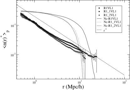
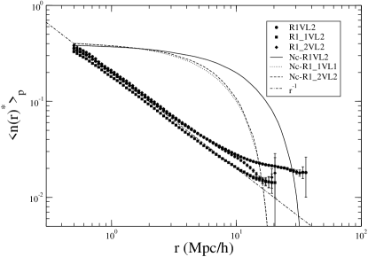
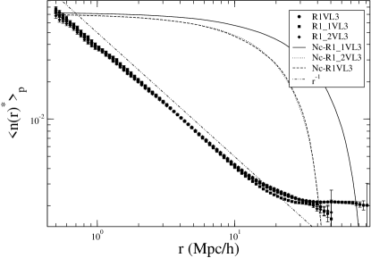
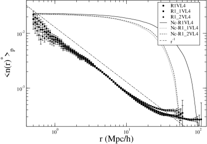
Let us now discuss the situation in some details. As already mentioned the average computed by Eq.7 is made by changing, at each scale $r$ the number $N_{c}(r)$ of points which do contribute. This scale-dependency follows from the requirement that only those points for which, when chosen as centers of a sphere of radius $r$, the volume does not overlap or intersect the boundaries of the sample. In this way, in a sample of size $R_{s}$, when $r\ll R_{s}$ almost all points will contribute to the average, while when $r\rightarrow R_{s}$ only those points lying close to the center of the volume will be taken into account in the average. Hence at large scales the average is performed on a number of points which exponentially decays when $r\rightarrow R_{s}$. In Figs.13-16 we show the behavior of the number of centers $N_{c}(r)$ as function of scale, normalized to an arbitrary factor for seek of clarity. The normalization is simple because at small scales $N_{c}(r)=N$ where $N$ is the number of points contained in a given VL sample: in fact at such small scales all points contribute to the statistics. One may note at a scale comparable but smaller than the sample size there is an abrupt decay of this quantity: this means that only few points contribute to the average at large scales.

That systematic fluctuations are more important than statistical ones, can be noticed from the behavior of the conditional density in Figs.13-16 by comparing the behaviors in the original sample (e.g. R1VL1) and in the two separate subsamples (e.g. R1$\_$1VL1 and R1$\_$2VL1). When the distance scale approaches the boundaries of the samples one may note that there are systematic variations which are larger than the (small) error bars derived from Eq.8. As already mentioned, in some cases there is an evidence for a more flatter behavior while in other cases instead the conditional density show a decay up to the sample boundaries which is slower than at smaller scales. This situation puts a serious warning for the interpretation of the large scale tail of the conditional density. The question is how to quantify the regime where systematic fluctuations are important and may affect the behavior of the conditional density.

One may define a criterion for the statistical robustness of the volume average, by imposing for example $N_{c}(r)$ to be larger than a certain value. While this can certainly give an useful indication, the problem of the volume average is more subtle. In fact when $r\rightarrow R_{s}$ there can be sufficiently enough points for $N_{c}(r)$ to be larger than a given pre-defined value: however it may happen that all these points lie, for example, in a cluster located close to the sample center. In this situation the volume average is not properly performed, in the sense that all points “see” almost the same volume.

A possibility to clarify such a situation has been proposed by Joyce et al. (1999). One may compute the average distance between the $N_{c}(r)$ centers at the scale $r$:

$$R_{c}(r)=\frac{1}{N_{c}(r)(N_{c}(r)-1)}\sum_{i,j=1}^{N_{c}(r)}|\@vec{r}_{i}-\@vec{r}_{j}|$$ (10)

where $\@vec{r}_{i}$ and $\@vec{r}_{j}$ are two of the $N_{c}(r)$ points. A criterion for statistical validity of the volume average is then

$$R_{c}\geq 2\times r$$ (11)

which implies that the average distance between sphere centers if larger than twice the scale at which the conditional density is computed, assuring in this way the independence of the different terms in the average. The values of $R_{c}$ for the different samples is reported in Tab.3 and this length-scale is indicated as a vertical line in Figs.9-12. In practice all samples show an $R_{c}$ smaller than 40 Mpc/h with the exception of R1VL3 and R1VL4 for which $R_{c}=54,\ 65;$ Mpc/h respectively. Hoverer in these two samples the conditional density does behave differently at large scales (see Fig.17), in the sense that the change of slope occurs at different scales and thus at a different value average density.

Figure 17: Conditional density in spheres in the R1VL3 and R1VL4 samples, normalized to have the same amplitude at 1 Mpc/h. One may see that the large scale behavior ($r>$30 Mpc/h) is different due to the effect of systematic fluctuations.

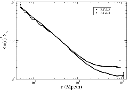
Thus it is very hard to conclude about the correlation properties at such large scales.

However we note that there is enough evidence that the signal is smoother on scales $>$ 40 Mpc/h and that sample-to-sample fluctuations or the variations in radial counts (discussed in Section 2) are smaller, thus indicating a tendency toward a more uniform distribution. However these data do not support unambiguously a clear evidence in favor of homogeneity at scales of order $70$ Mpc/h, as Hogg et al. (2005) found by analyzing the LRG sample, because the change in correlation properties occurs at scales comparable to the scales $R_{s}$ and $R_{c}$. We conclude that these data support an evidence for a change of slope, with a clear tendency for $\gamma<1$, but with undefined value.

These tests indicate that the availability of larger samples, provided, for example, by DR5, will allow one to understand these systematic variations. Particularly we may see that to study scales of order 100 Mpc/h, samples with $R_{s}\approx$ 300 Mpc/h are needed. However the full SDSS data will provide us with such large and complete catalogs.

4 Correlation properties of cosmological N-body simulations

Gravitational clustering in the regime of strong fluctuations is usually studied through gravitational N-body simulations. The particles are not meant to describe galaxies but collision-less dark-matter mass tracers. During gravitational evolution complex non-linear dynamics make non-linear structures at small scales, while at large scales it occurs a linear amplification according to linear perturbation theory. Thus, while on large scales correlation properties do not change from the beginning — a part a simple linear scaling of amplitudes — at small scales non-linear correlations are built. Typically in these simulations non-linear clustering is formed up to scales of order of few Mpc.

At late times one can identify subsamples of points which trace the high density regions, and these would represent the sites for galaxy formation, whose statistical properties are ultimately compared with the ones found in galaxy samples.

In order to study this problem we consider the GIF galaxy catalog (Kauffmann et al. (1999)) constructed from a $\Lambda$CDM simulation run by the Virgo consortium (Jenkins et al. (1998)). The way in which this is done is to firstly identify the halos, which represent almost spherical structures with a power-law density profile from their center. The number of galaxies belonging to each halo is set proportional to the total number of points belonging to the halo to a certain power. This procedure identifies points lying in high density regions of the dark-matter particles. One may assign to each point a luminosity and a color on the basis of a certain criterion which is not relevant for what follows (see Sheth et al. (2001) and reference therein). The resulting catalog is divided into two subsamples based on “galaxy” color B-I as in Sheth et al. (2001): (brighter) red galaxies (for which B-I is redder than 1.8) and (fainter) blue galaxies (B-I bluer than 1.8).

In summary four samples of points may be considered: (i) the original dark matter particles with $N$=$256^{3}$ particles (ii) all galaxies with $N$=15445 (iii) blue galaxies with $N$=11023 and (iv) red galaxies with $N$=4422.

In order to understand the correlation properties in the sampled point distributions it is useful to study the behavior of the conditional density which, as already discussed, has a straightforward interpretation in terms of correlations: results are shown in Fig.18.

Figure 18: Conditional density for the four samples of points selected in the simulation: the original dark matter (DM) field, all “galaxies” (ALL), blue galaxies (BLUE) and red galaxies (RED). The conditional density for dark matter particles (DM) has been normalized arbitrarily. The reference dashed-dotted line has a slope $\gamma=1.7$. The dashed line with $\gamma=1$, corresponding to the slope measured in the galaxy samples is also reported.

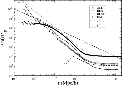
The red galaxies are responsible for the strong correlations observed in the full sample as the conditional density is almost the same as for all galaxies at small scales. At large scales there is instead a fast decrease as the sample average of red galaxies is smaller than the one of all galaxies (there are less objects). For red galaxies the sampling is local, i.e. their conditional density is (almost) invariant at small scales. Clearly, as there are globally less objects, the sample density of red galaxies is smaller than that of all galaxies. On the other hand blue galaxies present only some residual correlations at small scales, and they are more numerous than red galaxies.

The small scale properties of these distributions can be studied by analyzing the NN probability distribution (see Fig.19).

Figure 19: Nearest neighbors probability distribution for three point sets selected in the simulation (see discussion in the text): all “galaxies” (ALL), blue galaxies (BLUE) and red galaxies (RED).

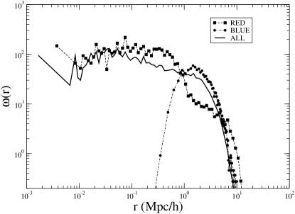
One may note that blue galaxies have a bell-shaped distribution, typical of the case where correlation are very weak. Instead red and all galaxies present almost the same function, with a long small-scale tail, which is the typical feature indicating the presence of strong two-point correlations (see discussion in Baertschiger and Sylos Labini, 2002). This situation is different from the one detected in the samples of DR4 as shown in Figs.1-4, where the NN probability distribution has the same shape for all different samples considered.

The main points we stress are the following:

• The slope of the conditional density in all the artificial samples considered here is different from $\gamma=1.0\pm 0.1$ measured in the real galaxy data. In particular for those mock samples (red galaxies, all galaxies and dark matter particles) where correlations are power-law, the slope is $\gamma=1.7\pm 0.1$ in the range [0.01,5] Mpc/h while a clear transition toward homogeneity occurs at scales of order 10 Mpc/h. These different slopes can be originated by the fact that we compare a measure in redshift space, in the case of real data, which can be affected by redshift distortions, with the mock catalogs where the conditional density has been measured in real space. We will examine this point in more detail in a forthcoming paper.

• Small scales properties, as detected by the NN probability distribution, are different in the real and artificial samples.

• The conditional densities of mock blue and red galaxies are different at all scales and blue galaxies show almost no correlations.

• Both mock red and blue galaxies show a well-defined transition to homogeneity at a scale of oder 10 Mpc/h. As we have already mentioned, this is not the behavior observed in the data. Particularly the range of non-linear structures seem to be much larger in the real data than in the simulations.

In conclusion, while the comparison between correlation properties of real galaxies and mock galaxy catalogs constructed from points selected in N-body simulations is usually performed by the analysis of the reduced two-point correlation function, here we have presented the comparison of the conditional density and of the NN probability distributions. We find that some important disagreement between data and simulations are evident when the behavior of these statistical quantities are considered. This is not the same conclusion that one may reach by analyzing the reduced correlation function $\xi(r)$: the reason is that in the estimation of $\xi(r)$ one uses the estimation of the sample average which introduces a finite-size effect which may affect both the amplitude and slope of this function (see e.g. Gabrielli et al., 2004 for a detailed discussion of this point). The estimation of the conditional density is less affected by finite-volume effects and the comparison between different sample is straightforward.

Note that the data are analyzed in redshift space and the simulations in real space. However given that velocities are typically smaller than $500$ km/s the difference between real and redshift space cannot be accounted by the effects of peculiar velocities on scales larger than 5 Mpc/h. The problem of the relation between real and redshift space, considering the finite size effects present when strong correlation characterize the data, has been discussed in Vasilyev, Baryshev & Sylos Labini (2006).

5 Discussion and Conclusions

Our main results are the following:

(i) In all VL samples we find that in the range of scales $0.5\leq r\mathrel{\hbox to0.0pt{\lower 3.0pt\hbox{$\mathchar 536\relax$}\hss}\raise 2.0pt\hbox{$\mathchar 316\relax$}}30$ Mpc/h the conditional density shows power-law correlation with a power-law index $\gamma=1.0\pm 0.1$. This result is in good agreement with the behavior found in other smaller samples by Sylos Labini et al. (1998), Joyce et al. (1999) and in the SDSS LRG sample by Hogg et al. (2005), and with the correlation properties measured by Vasilyev, Baryhsev & Sylos Labini (2006) in the 2dFGRS.

Note that we do not confirm the results of Zehavi et al. (2004) who found a departure from a power-law in the galaxy correlation function at a scale of order 1 Mpc/h: their analysis has been performed in real space while ours is in redshift space. In this range of scales nearest-neighbor correlation dominate the behavior of the conditional density and thus also of the reduced correlation function and for a detailed understanding of this regime a study of the nearest-neighbor is shown to be necessary.

In addition we do not find either a luminosity or color dependence of the galaxy the conditional density in the regime where the statistics is robust. In this respect Zehavi et al. (2005) have considered the behavior of the reduced two-point correlation function, and concluded that there is a color (luminosity) dependence of galaxy correlations. This apparent disagreement can be understood by considering that the reduced two-point correlation function can be strongly affected by finite-size effects in the regime where the conditional density presents power-law correlations (see discussion, e.g. in Joyce et al., 2005). Moreover results by Zehavi et al. (2005) have been obtained in real space: in Vasilyev, Baryhsev & Sylos Labini (2006) we discussed the kind of finite size effects which perturb the estimation of $\xi(r)$ when the conditional density has power-law correlations.

(ii) In the range $30\mathrel{\hbox to0.0pt{\lower 3.0pt\hbox{$\mathchar 536\relax$}\hss}\raise 2.0pt\hbox{$\mathchar 316\relax$}}r\mathrel{\hbox to0.0pt{\lower 3.0pt\hbox{$\mathchar 536\relax$}\hss}\raise 2.0pt\hbox{$\mathchar 316\relax$}}100$ Mpc/h the situation is less clear: as we discussed finite volume effects are important in this range of scales and systematic unaveraged fluctuations may affect the results. We have presented several tests to show the role of finite volume effects and to determine the range of scales where they perturb the estimation of the conditional density, finding that in all but two samples the volume average is properly performed up to $R_{c}\approx 40$ Mpc/h. In the remaining two samples we have shown that systematic fluctuations persist up to their boundaries $R_{s}$.

Thus in the range $30\mathrel{\hbox to0.0pt{\lower 3.0pt\hbox{$\mathchar 536\relax$}\hss}\raise 2.0pt\hbox{$\mathchar 316\relax$}}r\mathrel{\hbox to0.0pt{\lower 3.0pt\hbox{$\mathchar 536\relax$}\hss}\raise 2.0pt\hbox{$\mathchar 316\relax$}}100$ Mpc/h we find evidences for more uniform distribution and hence a smaller power law index ($\gamma<1$) in the conditional density. This is a stable result in all samples considered. However a detailed analysis of the behavior of the conditional density in all samples does not allow us to conclude neither that there is definitive crossover to homogeneity at a scales of order 70 Mpc/h as Hogg et al. (2005) have concluded by considering the LRG sample, nor that there is a change of power-law index beyond 30 Mpc/h which remain stable up to samples limit, i.e. up to 100 Mpc/h. Both possibilities are still open and will be clarified by forthcoming data releases of SDSS as the solid angle is going to sensibly grow.

(iii) The comparison of mock galaxy catalogs constructed from particle distributions extracted from cosmological N-body simulations with real galaxy data outlines a problematic situation. From the one hand we have discussed the fact that the slope of the conditional density in latter case is different from the one measured in real catalogs. On the other hand we have also stressed that when constructing artificial galaxy samples from dark matter particles in N-body simulations, there are different behaviors in the conditional density according to the different selection criteria used, and thus on the different way to assign “luminosity” and “color” to the artificial galaxies. In any case, this behavior is not in agreement with the data, as in all samples here analyzed, the same slope in the conditional density is measured. The same situation is present when the NN probability distribution is considered. Then in N-body simulations structures are sensibly smaller than in real data, as shown by the definitive crossover to homogeneity at about 10 Mpc/h found in N-body particle distribution, contrary to the galaxy case where the crossover may happen on much larger scales of order 100 Mpc/h.

It is worth noticing that we have used a very conservative statistical analysis which introduces an important constraints on the way we treat the data. For example if the distribution would have been uniform on scales smaller than the actual sample sizes, the conditional density estimation can be done for all points in the sample, even on large scales, not just the points near the center of the sample, because it can be assumed that volume outside the survey region is statistically similar to volume inside. This is the standard approach with conventional two-point statistics in the literature. On the other hand we have used, for example, periodic boundary conditions in the analysis of artificial simulations, as in this case the distribution is periodic, beyond the simulation box, by construction. However, as we do not know whether this is case for galaxy distribution, and actually we would like to test this point, we have used more conservative statistics to analyze the real data. This, instead of being a limitation, allow us to derive results about galaxy correlation properties which are unbiased by finite size effects. Indeed, when using less conservative methods, one is implicitly making the assumption that finite size effects, induced by long range correlations in the galaxy distribution, are negligible. Here we instead test that this is the case in the data we consider and actually we find evidence that, because of the long range nature of galaxy correlations, there are subtle finite size effects which should then put a serious warning on the use of less conservative statistical methods. Having used a more conservative statistics we are able to obtain results which are less biased by finite size effects (which ultimately appear from the presence of large fluctuations represented by large scale structures) with respect to the ones derived by a statistical analysis which makes use of some untested assumptions to derive its results. For example we get that the exponent of the conditional density is -1 instead of -1.7 as derived through a more “relaxed” analysis, at the same scales. The measurements of the conditional density has been performed in real space in the mock catalogs and in redshift space in the real samples, and this can be the origin of the different values of the correlation exponents. Whether this is case, or a finite size effect is playing a crucial role will be studied in a forthcoming paper.

Finally we would like to briefly discuss our results in relation to theoretical models of fluctuations in standard cosmologies. It has been shown (see e.g. Gabrielli et al. 2004) that the only feature of the primordial correlations, defined in theoretical models like the cold dark matter (CDM) one, which can be detected in galaxy data is represented by the large scale tail of the reduced correlation function. In fact, in terms of correlation function $\xi(r)$ CDM models presents the following behavior: it is positive at small scales, it crosses zero at a certain scale and then it is negative approaching zero with a tail which goes as $r^{-4}$ in the region corresponding to $P(k)\sim k$ (see e.g. Gabrielli et al. 2004). The super-homogeneity (or Harrison-Zeldovich) condition says that the volume integral over all space of the correlation function is zero

$$\int_{0}^{\infty}d^{3}r\xi(r)=0\;.$$ (12)

This means that there is a fine tuned balance between small-scale positive correlations and large-scale negative anti-correlations. This is the behavior that one would like to detect in the data in order to confirm inflationary models. Up to now this search has been done through the analysis of the galaxy power spectrum (PS) which should scale as $P(k)\sim k$ at small $k$ (large scales). No observational test of this behavior has been provided yet. However for this case one should consider an additional complication.

In standard models of structure formation galaxies result from a sampling of the underlying CDM density field: for instance one selects only the highest fluctuations of the field which would represent the locations where galaxy will eventually form. It has been shown that sampling a super-homogeneous fluctuation field changes the nature of correlations (Durrer et al., 2003). The reason for this can be found in the property of super-homogeneity of such a distribution: the sampling necessarily destroys the surface nature of the fluctuations, as it introduces a volume (Poisson-like) term in the mass fluctuations, giving rise to a Poisson-like PS on large scales $P(k)\sim$ constant. The “primordial” form of the PS is thus not apparent in that which one would expect to measure from objects selected in this way. This conclusion should hold for any generic model of bias and its quantitative importance has to be established in any given model (Durrer et al., 2003).

On the other hand one may show (Durrer et al., 2003) that the negative $r^{-4}$ tail in the correlation function does not change under sampling: on large enough scales, where in these models (anti) correlations are small enough, the biased fluctuation field has a correlation function which is linearly amplified with respect to the underlying dark matter correlation function. For this reason the detection of such a negative tail would be the main confirmation of models of primordial density field. This will be possible if firstly a clear determination of the homogeneity scale will be obtained, and then if the data will be statistically robust enough to allow the determination of the correlation when it is $\xi(r)\ll 1$. While Eiseinstein et al. (2005) claimed to have measured that $\xi(r)\approx 0.01$ at scales of order 100 Mpc/h in a sample of SDSS LRG galaxies, here we cannot confirm these results as our analysis does not extend to such large scales with a robust statistics. However from the large fluctuations observed, for example in the behavior of the radial counts and in sample-to-sample variations of the conditional density at such large scales, we conclude that this result deserves more studies, and perhaps much larger samples, to be confirmed.

References

- (1) Adelman-McCarthy J.K. et al. astro-ph/0507711
- (2) Baryshev, Yu., Teerikorpi P., 2005, Bull. Special Astrophys. Obs in print astro-ph/0505185
- Baertschiger & Sylos Labini (2004) Baertschiger T. & Sylos Labini F., 2004, Phys.Rev.D, 69, 123001-1
- (4) Blanton, M.R., et al., 2001, AJ 121 2358
- Durrer et al. (2003) Durrer, R., Gabrielli, A., Joyce, M., Sylos Labini, F., 2003, ApJ 585, L1
- Eisenstein et al. (2005) Eisenstein, D.J., et al., 2005, ApJ 633, 560
- (7) Gabrielli A., Sylos Labini F., Joyce M., Pietronero L., Statistical physics for cosmic structures, Springer Verlag (2004)
- (8) Kerscher, M., A&A, 1999, 343, 333,
- (9) Hogg, D.W., Eistenstein, D.J., Blanton M.R., Bahcall N.A, Brinkmann, J., Gunn J.E., Schneider D.P. 2005 ApJ, 624, 54
- Kauffmann et al. (1999) Kauffmann G., Colberg J., Diaferio A., White S.D.M., 1999, MNARS, 303, 188
- Jenkins et al. (1998) Jenkins, A., et al., 1998, ApJ, 499, 20
- (12) Joyce, M., Montuori, M., Sylos Labini, F., 1999, ApJ, 514, L5
- (13) Joyce, M., Sylos Labini, F., Gabrielli, A., Montuori, M., Pietronero, L., 2005 A&A 443, 11
- (14) Nichol, R.C., et al. astro-ph/0602548
- Pietronero (1987) Pietronero, L., 1987, Physica A, 144, 257
- Sheth et al. (2001) Sheth, R.K., Diaferio, A., Hui, L., Scoccimarro, R., 2001 MNRAS, 326, 463
- (17) Strauss, M.A. et al. 2002, AJ, 124, 1810
- Sylos Labini, Montuori & Pietronero (1998) Sylos Labini, F., Montuori, M. & Pietronero, L., 1998, Phys.Rep.,293, 66
- (19) Vasilyev, N.L., Baryshev, Yu. V., Sylos Labini, F., 2006 A&A 447, 431
- Zehavi et al. (2004) Zehavi, I., et al. 2004 ApJ, 608, 16
- Zehavi et al. (2005) Zehavi, I., et al. 2005 ApJ, 630, 1