BETOCS using the 157 gold SNe Ia Data : Hubble is not humble

Abstract

The type Ia supernovae observational data is one of the most important in observational cosmology nowadays. Here we present the first public version of BETOCS (BayEsian Tools for Observational Cosmology using SNe Ia), which is a powerful and high productivity tool aimed to help the theoretical physicist community investigate cosmological models using type Ia supernovae (SNe Ia) observational data. BETOCS is applied to the generalized Chaplygin gas model (GCGM), traditional Chaplygin gas model (CGM) and $\Lambda$CDM, ranging from 5 to 3 free parameters, respectively. The “gold sample” of 157 supernovae data is used. It is shown that the Chaplygin gas scenario is viable (in most cases the $\Lambda$CDM is disfavoured) and the quartessence scenario (that unifies the description for dark matter and dark energy) is favoured. The Hubble parameter ($H_{0}$) is important and should not be fixed and it can be estimated or marginalized with or without the Hubble Space Telescope prior.

PACS number(s): 98.80.Bp, 98.80.Es, 04.60.Gw

1 Introduction

The type Ia supernovae (SNe Ia) observational data has forced us to discard or change the majority of theoretical cosmological models supposed to be correct until the second half of the last decade [1, 2]. The crossing of the SNe Ia statistics with other observational data, like the anisotropy of the cosmic microwave background radiation (CMBR) [3], gravitational lensing [4, 5], the X-ray gas mass fraction of galaxy clusters [6], etc, leads to a scenario where the matter content of the Universe is described by an unclustered component of negative pressure, the dark energy, and a clustered component of zero pressure, the cold dark matter.

There are many candidate for dark energy, the most natural seems to be the cosmological constant [7], since it can be connected with the vacuum energy in quantum field theory [8], but the small value resulting from observations for the energy density of the cosmological constant term yields a discrepancy of about $120$ orders of magnitude with the theoretically predicted value [9]. Among many other possibilities, for example there is the quintessence model with scalar fields [10, 11].

Here we will focus on the Chaplygin gas models (CGM) [12, 13, 14, 15]. It is based on a string inspired configuration that leads to a specific equation of state where pressure is negative and varies with the inverse of the density [16]. This model has been generalized, giving birth to the generalized Chaplygin gas model (GCGM), where now the pressure varies with a power of the inverse of the density [15]. These proposals have many advantages, among which we can quote the following: in spite of presenting a negative pressure, the sound velocity is positive, what assures stability [17]; these models can unify the description of dark energy and dark matter, since the fluid can clusters at small scale, remaining a smooth component at large scales [15]; the CGM has an interesting connection with string theory [16]. Some criticisms have been addressed to the GCGM (CGM) mainly connected with its features related to the power spectrum for the agglomerated matter [18]. However, in our opinion, this specific criticism is not conclusive, since the introduction of baryons may alleviate the objections presented against the cosmological scenarios based on the GCGM (GCM) [19].

The GCGM (Generalized Chaplygin Gas Model) is defined as a perfect fluid with an equation of state given by

$$p=-\frac{A}{\rho^{\alpha}}\quad,$$ (1)

where $A$ and $\alpha$ are constants. When $\alpha=1$ we re-obtain the equation of state for the CGM (Chaplygin Gas Model), the traditional Chaplygin gas model. See refs. [20, 21, 22] for more detailed definitions of the Chaplygin gas models used in the present work.

All free parameters for each model are considered. In the case of the GCGM there are five free parameter: the Hubble constant $H_{0}$; the equation of state parameter $\alpha$; the “sound velocity” related parameter $\bar{A}$; the density parameter for the pressureless matter $\Omega_{m0}$; the density parameter for the Chaplygin gas $\Omega_{c0}$ (or alternatively the density parameter for the curvature density of the Universe $\Omega_{k0}$). For the CGM, the number of parameters reduce to four, since $\alpha=1$. We also consider the $\Lambda$CDM, where the number of parameters reduce to three: $H_{0}$, $\Omega_{m0}$ and $\Omega_{c0}$ (alternatively, $\Omega_{k0}$).

One important point is how to perform this statistical analysis: the final conclusions may, in some cases, depend on the statistical framework (Bayesian, frequentist, etc.), as well as on the parameters that are allowed to be free, and how these parameters are constrained (through a joint probability for two parameters, minimizing the error function or through a marginalization of all parameters excepted one, etc.). In some cases, the different procedures adopted may lead to quite different conclusions on the best value for a given set of parameters. The choice of the observational data sample may of course be important as well.

The present work is intended to :

1. Announce the first public version of BETOCS (BayEsian Tools for Observational Cosmology using SNe Ia [23]), which is a powerful and high productivity tool aimed to help the theoretical physicist community investigate cosmological models using type Ia supernovae (SNe Ia) observational data. BETOCS is a freeware and open source tool written in the Mathematica [24] language. The Mathematica notebooks of BETOCS contain documentation, source code and practical examples with textual and graphical outputs.

2. Emphasize that fixing $H_{0}$ is not acceptable, yielding arbitrary parameter estimations and usually bad best-fittings. On the other hand, the HST (Hubble Space Telescope) prior [25] for $H_{0}$ implies minor effects on all best-fittings and parameter estimations (as shown here comparing the tables with flat and HST priors for $H_{0}$), so its use is just a matter of choice. Nevertheless, it is recommended to use the HST prior as it is standard when using other observational cosmological data (X-ray gas mass fraction, etc).

3. Continue the work of refs. [20, 21, 22] and show a very complete view and analysis of the Chaplygin gas models (generalized and traditional) using SNe Ia. The present work specially fixes an error on ref. [20] when calculating the best-fittings and parameter estimations for non-flat Universes ( $\Omega_{k0}\neq 0$), due to an earlier version of BETOCS with wrong optimization code. B$\frac{{}}{{}}$ut the side-effects of this error were not critical, just worsening some positive features.

The best-fitting parameters and the parameter estimations were calculated for each case of GCGM, CGM or $\Lambda$CDM using a corresponding BETOCS (BayEsian Tools for Observational Cosmology using SNe Ia [23]) notebook (written in Mathematica [24] language) containing the : definitions of the theoretical cosmological model, reading of the observational SNe Ia data, $\chi^{2}$ definition, Bayesian tools library, calculation of the Bayesian PDF, global maximization of PDF, PDF visualization in $3$ dimensions (if available), PDF visualization and analysis in $2$ dimensions and finally PDF visualization in $1$ dimension with parameter estimation. This article does not include all the graphics and analyses of the BETOCS notebooks, but some of them are available on the Internet site of the BETOCS project [23].

This paper is organized as follows. In section 2 we detail the best-fitting analysis using BETOCS, with many results presented in tables. Section 3 explains how the parameter estimations are made using BETOCS, such that a detailed Bayesian analysis is performed for each independent and dependent parameter, with the results shown in many tables and figures. The conclusions are discussed in section 4.

2 Best-fitting parameters using BETOCS

In order to compare the theoretical results with the observational data, the first step in this sense is to compute the quality of the fitting through the least squared fitting quantity $\chi^{2}$. In the case of flat priors for all independent parameters of the theoretical cosmological model, we get

$$\chi^{2}=\sum_{i}\frac{\left(\mu_{0,i}^{o}-\mu_{0,i}^{t}\right)^{2}}{\sigma_{\mu_{0},i}^{2}}\quad.$$ (2)

In this expression, $\mu_{0,i}^{o}$ is the distance moduli observationaly measured for each supernova of the $157$ gold SNe Ia dataset [26], $\mu_{0,i}^{t}$ is the value calculated through the theoretical cosmological model, $\sigma_{\mu_{0},i}^{2}$ is the measurement error and includes the dispersion in the distance modulus due to the dispersion in galaxy redshift due to peculiar velocities, following ref. [26]. It is useful to define $\chi_{\nu}^{2}$ : $\chi^{2}$ divided by the number of degrees of freedom of the observational data, i.e., the number of SNe Ia, here $157$.

As we also want to compare the fitting and estimation of the parameters without priors and with the HST (Hubble Space Telescope) prior [25] for $H_{0}$, then the $\chi^{2}$ used for the calculations with the HST prior is simply

$$\chi^{2}=\sum_{i}\frac{\left(\mu_{0,i}^{o}-\mu_{0,i}^{t}\right)^{2}}{\sigma_{\mu_{0},i}^{2}}+\frac{(H_{0}-72)^{2}}{8^{2}}\quad.$$ (3)

GCGM					$k=0$,	$k=0$,
with		$k=0$	$\Omega_{m0}=0$	$\Omega_{m0}=0.04$	$\Omega_{m0}=0$	$\Omega_{m0}=0.04$
$\chi_{\nu}^{2}$	$1.1075$	$1.1094$	$1.1075$	$1.1081$	$1.1094$	$1.1096$
$\alpha$	$7.70$	$2.83$	$7.53$	$7.75$	$2.83$	$3.07$
$H_{0}$	$65.03$	$65.12$	$65.03$	$64.98$	$65.12$	$65.09$
$\Omega_{k0}$	$0.177$	$0$	$0.173$	$0.153$	$0$	$0$
$\Omega_{m0}$	$0.000$	$0.000$	$0$	$0.04$	$0$	$0.04$
$\Omega_{c0}$	$0.823$	$1.000$	$0.827$	$0.807$	$1$	$0.96$
$\bar{A}$	$0.996$	$0.929$	$0.996$	$0.998$	$0.929$	$0.949$
$t_{0}$	$13.53$	$13.55$	$13.53$	$13.53$	$13.55$	$13.55$
$q_{0}$	$-0.819$	$-0.893$	$-0.822$	$-0.785$	$-0.893$	$-0.866$
$a_{i}$	$0.786$	$0.753$	$0.786$	$0.777$	$0.753$	$0.751$

Table 1: The best-fitting parameters, i.e., when $\chi_{\nu}^{2}$ is minimum, for each type of spatial section and matter content of the generalized Chaplygin gas model. $H_{0}$ is given in $km/M\!pc.s$, $\bar{A}$ in units of $c$, $t_{0}$ in $Gy$ and $a_{i}$ in units of $a_{0}$.

GCGM					$k=0$,	$k=0$,
with		$k=0$	$\Omega_{m0}=0$	$\Omega_{m0}=0.04$	$\Omega_{m0}=0$	$\Omega_{m0}=0.04$
$\chi_{\nu}^{2}$	$1.1122$	$1.1140$	$1.1122$	$1.1129$	$1.1140$	$1.1143$
$\alpha$	$7.73$	$2.96$	$7.27$	$7.57$	$2.96$	$3.22$
$H_{0}$	$65.11$	$65.20$	$65.11$	$65.06$	$65.20$	$65.17$
$\Omega_{k0}$	$0.170$	$0$	$0.162$	$0.143$	$0$	$0$
$\Omega_{m0}$	$0.000$	$0.000$	$0$	$0.04$	$0$	$0.04$
$\Omega_{c0}$	$0.830$	$1.000$	$0.838$	$0.817$	$1$	$0.96$
$\bar{A}$	$0.996$	$0.935$	$0.995$	$0.997$	$0.935$	$0.954$
$t_{0}$	$13.53$	$13.54$	$13.52$	$13.53$	$13.54$	$13.54$
$q_{0}$	$-0.826$	$-0.902$	$-0.832$	$-0.794$	$-0.902$	$-0.874$
$a_{i}$	$0.785$	$0.754$	$0.784$	$0.776$	$0.754$	$0.752$

Table 2: The best-fitting parameters, i.e., when $\chi_{\nu}^{2}$ is minimum, for each type of spatial section and matter content of the generalized Chaplygin gas model using the HST prior. $H_{0}$ is given in $km/M\!pc.s$, $\bar{A}$ in units of $c$, $t_{0}$ in $Gy$ and $a_{i}$ in units of $a_{0}$.

CGM					$k=0$,	$k=0$,
with		$k=0$	$\Omega_{m0}=0$	$\Omega_{m0}=0.04$	$\Omega_{m0}=0$	$\Omega_{m0}=0.04$
$\chi_{\nu}^{2}$	$1.1119$	$1.1141$	$1.1119$	$1.1121$	$1.1141$	$1.1147$
$H_{0}$	$64.96$	$64.73$	$64.96$	$64.95$	$64.73$	$64.70$
$\Omega_{k0}$	$-0.149$	$0$	$-0.149$	$-0.160$	$0$	$0$
$\Omega_{m0}$	$0.000$	$0.000$	$0$	$0.04$	$0$	$0.04$
$\Omega_{c0}$	$1.149$	$1.000$	$1.149$	$1.120$	$1$	$0.96$
$\bar{A}$	$0.806$	$0.811$	$0.806$	$0.825$	$0.811$	$0.834$
$t_{0}$	$13.91$	$14.01$	$13.91$	$13.92$	$14.01$	$14.03$
$q_{0}$	$-0.815$	$-0.717$	$-0.815$	$-0.807$	$-0.717$	$-0.701$
$a_{i}$	$0.702$	$0.699$	$0.702$	$0.699$	$0.699$	$0.695$

Table 3: The best-fitting parameters, i.e., when $\chi_{\nu}^{2}$ is minimum, for each type of spatial section and matter content of the traditional Chaplygin gas model. $H_{0}$ is given in $km/M\!pc.s$, $\bar{A}$ in units of $c$, $t_{0}$ in $Gy$ and $a_{i}$ in units of $a_{0}$.

CGM					$k=0$,	$k=0$,
with		$k=0$	$\Omega_{m0}=0$	$\Omega_{m0}=0.04$	$\Omega_{m0}=0$	$\Omega_{m0}=0.04$
$\chi_{\nu}^{2}$	$1.1167$	$1.1193$	$1.1167$	$1.1170$	$1.1193$	$1.1200$
$H_{0}$	$65.04$	$64.80$	$65.04$	$65.02$	$64.80$	$64.76$
$\Omega_{k0}$	$-0.158$	$0$	$-0.158$	$-0.170$	$0$	$0$
$\Omega_{m0}$	$0.000$	$0.000$	$0$	$0.04$	$0$	$0.04$
$\Omega_{c0}$	$1.158$	$1.000$	$1.158$	$1.130$	$1$	$0.96$
$\bar{A}$	$0.808$	$0.813$	$0.808$	$0.827$	$0.813$	$0.836$
$t_{0}$	$13.91$	$14.02$	$13.91$	$13.93$	$14.02$	$14.04$
$q_{0}$	$-0.824$	$-0.720$	$-0.824$	$-0.816$	$-0.720$	$-0.703$
$a_{i}$	$0.701$	$0.697$	$0.701$	$0.698$	$0.697$	$0.693$

Table 4: The best-fitting parameters, i.e., when $\chi_{\nu}^{2}$ is minimum, for each type of spatial section and matter content of the traditional Chaplygin gas model using the HST prior. $H_{0}$ is given in $km/M\!pc.s$, $\bar{A}$ in units of $c$, $t_{0}$ in $Gy$ and $a_{i}$ in units of $a_{0}$.

	$\Lambda CDM$		$\Lambda CDM$ :		$\Lambda CDM$ :		$\Lambda CDM$ :
			$k=0$		$\Omega_{m0}=0$		$\Omega_{m0}=0.04$
$H_{0}$ Prior	$flat$	$HST$	$flat$	$HST$	$flat$	$HST$	$flat$	$HST$
$\chi_{\nu}^{2}$	$1.1149$	$1.1199$	$1.1279$	$1.1337$	$1.2002$	$1.2068$	$1.1882$	$1.1946$
$H_{0}$	$64.85$	$64.93$	$64.32$	$64.39$	$63.78$	$63.86$	$63.90$	$63.98$
$\Omega_{k0}$	$-0.437$	$-0.447$	$0$	$0$	$0.803$	$0.795$	$0.692$	$0.684$
$\Omega_{m0}$	$0.459$	$0.460$	$0.309$	$0.306$	$0$	$0$	$0.04$	$0.04$
$\Omega_{\Lambda}$	$0.978$	$0.987$	$0.691$	$0.694$	$0.197$	$0.205$	$0.268$	$0.276$
$t_{0}$	$14.83$	$14.85$	$14.87$	$14.88$	$16.85$	$16.88$	$16.10$	$16.13$
$q_{0}$	$-0.749$	$-0.757$	$-0.537$	$-0.540$	$-0.197$	$-0.205$	$-0.248$	$-0.256$
$a_{i}$	$0.617$	$0.615$	$0.607$	$0.605$	$0$	$0$	$0.421$	$0.417$

Table 5: The best-fitting parameters, i.e., when $\chi_{\nu}^{2}$ is minimum, for each type of spatial section and matter content of the $\Lambda$CDM model using flat and HST priors. $H_{0}$ is given in $km/M\!pc.s$, $t_{0}$ in $Gy$ and $a_{i}$ in units of $a_{0}$.

In tables 1 and 2 the values of the parameters for the minimum $\chi_{\nu}^{2}$ ($\chi^{2}$ divided by the number of SNe Ia) are given for the GCGM with five free parameters $(\alpha,H_{0},\Omega_{m0},\Omega_{c0},\bar{A})$ and for other cases where the pressureless mater, the curvature or both are fixed, respectively using the flat prior for $H_{0}$ and the HST (Hubble Space Telescope) prior for $H_{0}$. Analogously, the same estimations are presented in tables 3 and 4 for the CGM, for up to four free parameters $(H_{0},\Omega_{m0},\Omega_{c0},\bar{A})$, and in table 5 for the $\Lambda$CDM, for up to three free parameters $(H_{0},\Omega_{m0},\Omega_{\Lambda})$.

It is important to emphasize that, for each case, all free independent parameters are considered simultaneously to obtain the minimum of $\chi_{\nu}^{2}$. So, for example assuming the GCGM, if we ask for the best simultaneous values of $(\alpha,H_{0},\Omega_{m0},\Omega_{c0},\bar{A})$ then the answer is given by the first column of table 1. However, in this example, asking for the best value of $\alpha$ by weighing (marginalizing or integrating) all possible values of $(H_{0},\Omega_{m0},\Omega_{c0},\bar{A})$ yields the estimation in the first column of table 6, whose peak of $0.59$ for $\alpha$ is totally different from $7.70$ as best-fitting parameter ! The parameter estimation issue is addressed by the Bayesian statistics of the next section, not by best-fitting in $n$-dimensional parameter space.

Each column of these best-fitting tables was calculated using a corresponding BETOCS [23] notebook. The minimization of $\chi_{\nu}^{2}$ is obtained in the following way : the initial global minimum taken from the $n$-dimensional discrete parameter space (see next section) is used as initial value to search for the local minimum of $\chi_{\nu}^{2}$ by using the function FindMinimum of the software Mathematica [24].

Note that the minimum values for $\chi^{2}$ using the “gold sample” are worse (i.e., higher, from $1.11$ to $1.20$) than the corresponding ones (between $0.74$ and $0.77$) using the restricted sample of $26$ supernovae [21, 22] (which have excellent quality). While the minima for $\chi^{2}$ are always slightly higher when the HST prior is used (because the HST prior peak is far from the best-fitting $H_{0}$), yielding best-fitting parameter values with minor changes. Other important results : the parameter $\alpha$ is usually much bigger than $1$, $\bar{A}$ is often near unity, $\Omega_{k0}$ is not far from $0$ suggesting a flat spatial section (except for $\Lambda$CDM), $\Omega_{m0}$ being null recovers the quartessence [13, 27] scenario (except for $\Lambda$CDM), $q_{0}$ and $a_{i}$ point to an accelerating Universe today with an age $t_{0}$ of approximately $14$ Gy. But these results must be compared with a more complete statistical analysis to be presented below.

3 Parameter estimations using BETOCS

Following the previous works [20, 21, 22], the Bayesian statistical analysis is employed here instead of the more usual frequentist (or standard or traditional) statistics. The Bayesian statistics emphasizes considering only the (observational) data you have, rather than simulating an infinite space of data, which is an advantage. On the other hand, the Bayesian marginalization process is computationally time-consuming if the number of parameters of the theoretical model is large. For the case here, with a maximum of five free parameters and low number of data points (157 SNe Ia), the Bayesian approach is better suited than the frequentist statistics. See Refs. [28, 29, 30, 31] for discussions about the frequentist versus Bayesian statistics and some applications in physics.

The probability of the set of distance moduli $\mu_{0}$ conditional on the values of a set of parameters $\{p_{i}\}$ is given by the Gaussian :

$$p(\mu_{0}|\{p_{i}\})\propto\exp\biggr{(}-\frac{\chi^{2}}{2\,}\biggl{)}\quad.$$ (4)

This probability distribution must be normalized. Evidently, when, for a set of values of the parameters, the $\chi^{2}$ is minimum the probability is maximum. This is a valuable information but is not enough to constraint the parameters.

From the probability distribution (4), a joint probability distribution for any subset of parameters can be obtained by integrating (marginalizing) on the remaining parameters, see refs. [21, 22]. So, in order to properly estimate a single parameter, the probability distribution must be marginalized on all other parameters, usually yielding a quite different result if we try to estimate the parameter in a two or three-dimensional parameter space. The reason is that, in such multidimensional parameter space, if a parameter has a large probability density but in a narrow region, the total contribution of this region may be quite small compared to other large regions which have small probability: in the marginalization process, this kind of high PDF region contributes little to the estimation of a given parameter.

Hence the estimation of a given parameter will be made by marginalizing on all other ones. A detailed Bayesian analysis of the independent and dependent parameters is shown in tables 6, 8 and 10 for GCGM, CGM and $\Lambda$CDM with flat prior for $H_{0}$, and in tables 7, 9 and 11 for GCGM, CGM and $\Lambda$CDM with the HST (Hubble Space Telescope) prior for $H_{0}$. Each column of these tables was calculated using a corresponding BETOCS [23] notebook (including the best-fitting calculations for the specific model).

The following estimation analyses will focus on the tables 6–11 and the accompanying figures.

3.1 Estimation of $H_{0}$ : Hubble is not humble

The predicted value of the Hubble constant today $H_{0}$ is the most robust one, with minor changes for the different models (GCGM, CGM and $\Lambda$DCM) and cases of fixed parameters. When comparing with ref. [20], $H_{0}$ is now slightly smaller.

Figure 1: The one-dimensional PDF for $H_{0}$. The thin line shows the HST (Hubble Space Telescope) prior, with the $1\sigma$ ($68.27\%$), $2\sigma$ ($95.45\%$) and $3\sigma$ ($99.73\%$) regions delimited by red, blue and green lines, respectively. The thick line shows a typical $H_{0}$ estimation from SNe Ia analysis in this article, clearly showing that the HST prior has much larger dispersion and its $2\sigma$ region includes the $H_{0}$ estimation from SNe Ia.

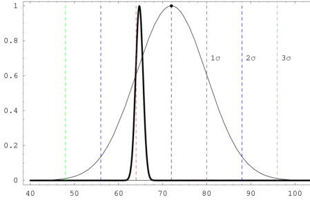
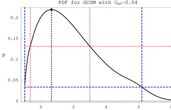
Figure 1 shows a typical $H_{0}$ estimation from SNe Ia analysis in this article, and the HST (Hubble Space Telescope) prior [25] for $H_{0}$, which has a much larger dispersion. The effect of the HST prior on the $H_{0}$ estimation is small : it slightly changes the shape PDF for $H_{0}$, the PDF peak moves increases (moves to the right) and there are some very  small changes on the left and right dispersions.

The minor effect of the HST prior can also be verified by comparing tables 6, 8 and 10 for GCGM, CGM and $\Lambda$CDM with flat prior for $H_{0}$ with tables 7, 9 and 11 for GCGM, CGM and $\Lambda$CDM with the HST (Hubble Space Telescope) prior for $H_{0}$.

It is important to emphasize that fixing $H_{0}$ is not acceptable as the n-dimensional PDF quite depends on the $H_{0}$ parameter. For $\Lambda$CDM as an example : $\chi_{\nu}^{2}$ is very high ($1.563$), $\Omega_{k0}=-0.890_{-0.241}^{+0.286}$ and many other totally different parameter estimations.

3.2 Estimation of $\alpha$

With respect to ref. [20], the peak values of $\alpha$ are slightly increased and the dispersion is also a little larger, for example, the GCGM now gives $\alpha=-0.59_{-0.41}^{+5.27}$. Imposing that the space is flat or fixing the pressureless matter lead to positive best values for $\alpha$. For example, the quartessence [13, 27] scenario ($\Omega_{m}=0$) predicts $\alpha=0.90^{+5.52}_{-1.83}$.

GCGM					$k=0$,	$k=0$,
with		$k=0$	$\Omega_{m0}=0$	$\Omega_{m0}=0.04$	$\Omega_{m0}=0$	$\Omega_{m0}=0.04$
$\alpha$	$-0.59_{-0.41}^{+5.27}$	$1.18_{-2.18}^{+4.22}$	$0.90_{-1.83}^{+5.52}$	$0.64_{-1.64}^{+5.55}$	$1.57_{-1.95}^{+5.09}$	$1.52_{-1.97}^{+4.76}$
$H_{0}$	$64.68_{-1.69}^{+1.73}$	$64.52_{-1.57}^{+1.64}$	$64.73_{-1.72}^{+1.74}$	$64.70_{-1.72}^{+1.75}$	$64.93_{-1.66}^{+1.55}$	$64.84_{-1.62}^{+1.54}$
$\Omega_{k0}$	$-0.251_{-0.694}^{+0.605}$	$0$	$0.065_{-0.833}^{+0.509}$	$0.025_{-0.827}^{+0.496}$	$0$	$0$
$\Omega_{m0}$	$0.000_{-0.000}^{+0.499}$	$0.000_{-0.000}^{+0.301}$	$0$	$0.04$	$0$	$0.04$
$\Omega_{c0}$	$1.012_{-0.489}^{+0.667}$	$1.000_{-0.301}^{+0.000}$	$0.935_{-0.509}^{+0.833}$	$0.935_{-0.496}^{+0.827}$	$1$	$0.96$
$\bar{A}$	$1.000_{-0.348}^{+0.000}$	$0.989_{-0.245}^{+0.011}$	$0.987_{-0.388}^{+0.012}$	$0.988_{-0.382}^{+0.012}$	$0.987_{-0.293}^{+0.013}$	$0.987_{-0.278}^{+0.012}$
$t_{0}$	$14.42_{-1.77}^{+2.51}$	$13.74_{-0.96}^{+1.76}$	$13.77_{-1.08}^{+2.39}$	$13.77_{-1.06}^{+2.82}$	$13.56_{-0.83}^{+1.34}$	$13.60_{-0.76}^{+1.40}$
$q_{0}$	$-0.730_{-0.328}^{+0.352}$	$-0.717_{-0.247}^{+0.305}$	$-0.750_{-0.399}^{+0.392}$	$-0.750_{-0.372}^{+0.399}$	$-0.928_{-0.114}^{+0.394}$	$-0.886_{-0.106}^{+0.369}$
$a_{i}$	$0.626_{-0.123}^{+0.184}$	$0.740_{-0.179}^{+0.073}$	$0.735_{-0.262}^{+0.121}$	$0.740_{-0.294}^{+0.108}$	$0.760_{-0.147}^{+0.069}$	$0.752_{-0.151}^{+0.072}$
$p(\alpha>0)$	$66.74\,\%$	$87.82\,\%$	$87.92\,\%$	$85.40\,\%$	$96.46\,\%$	$95.61\,\%$
$p(\alpha=1)$	$40.81\,\%$	$91.09\,\%$	$95.94\,\%$	$85.17\,\%$	$70.44\,\%$	$73.19\,\%$
$p(\Omega_{k0}<0)$	$79.05\,\%$	$-$	$49.21\,\%$	$55.18\,\%$	$-$	$-$
$p(\Omega_{k0}=0)$	$45.70\,\%$	$-$	$82.48\,\%$	$93.06\,\%$	$-$	$-$
$p(\bar{A}\neq 1)$	$0\,\%$	$59.15\,\%$	$100\,\%$	$100\,\%$	$100\,\%$	$100\,\%$
$p(q_{0}<0)$	$5.14\,\sigma$	$7.07\,\sigma$	$100\,\%$	$100\,\%$	$100\,\%$	$100\,\%$
$p(a_{i}<1)$	$5.26\,\sigma$	$7.49\,\sigma$	$100\,\%$	$5.56\,\sigma$	$100\,\%$	$100\,\%$

Table 6: The estimated parameters for the generalized Chaplygin gas model (GCGM) and some specific cases of spatial section and matter content. We use the Bayesian analysis to obtain the peak of the one-dimensional marginal probability and the $2\,\sigma$ credible region for each parameter. $H_{0}$ is given in $km/M\!pc.s$, $\bar{A}$ in units of $c$, $t_{0}$ in $Gy$ and $a_{i}$ in units of $a_{0}$.

GCGM					$k=0$,	$k=0$,
with		$k=0$	$\Omega_{m0}=0$	$\Omega_{m0}=0.04$	$\Omega_{m0}=0$	$\Omega_{m0}=0.04$
$\alpha$	$-0.57_{-0.43}^{+5.23}$	$1.24_{-2.24}^{+4.19}$	$0.93_{-1.85}^{+5.46}$	$0.67_{-1.66}^{+5.45}$	$1.63_{-1.96}^{+5.04}$	$1.57_{-1.98}^{+4.71}$
$H_{0}$	$64.78_{-1.70}^{+1.70}$	$64.61_{-1.57}^{+1.63}$	$64.83_{-1.74}^{+1.72}$	$64.80_{-1.74}^{+1.72}$	$65.00_{-1.65}^{+1.54}$	$64.92_{-1.62}^{+1.52}$
$\Omega_{k0}$	$-0.261_{-0.687}^{+0.602}$	$0$	$0.055_{-0.825}^{+0.503}$	$0.015_{-0.819}^{+0.491}$	$0$	$0$
$\Omega_{m0}$	$0.000_{-0.000}^{+0.499}$	$0.000_{-0.000}^{+0.297}$	$0$	$0.04$	$0$	$0.04$
$\Omega_{c0}$	$1.022_{-0.485}^{+0.661}$	$1.000_{-0.297}^{+0.000}$	$0.945_{-0.503}^{+0.825}$	$0.945_{-0.491}^{+0.819}$	$1$	$0.96$
$\bar{A}$	$1.000_{-0.345}^{+0.000}$	$0.989_{-0.240}^{+0.011}$	$0.987_{-0.384}^{+0.012}$	$0.988_{-0.378}^{+0.012}$	$0.987_{-0.286}^{+0.013}$	$0.987_{-0.271}^{+0.012}$
$t_{0}$	$14.43_{-1.78}^{+2.50}$	$13.74_{-0.95}^{+1.76}$	$13.77_{-1.09}^{+2.37}$	$13.77_{-1.06}^{+2.80}$	$13.48_{-0.66}^{+1.37}$	$13.49_{-0.62}^{+1.45}$
$q_{0}$	$-0.741_{-0.324}^{+0.351}$	$-0.717_{-0.251}^{+0.296}$	$-0.757_{-0.400}^{+0.386}$	$-0.764_{-0.366}^{+0.397}$	$-0.931_{-0.112}^{+0.385}$	$-0.888_{-0.104}^{+0.361}$
$a_{i}$	$0.623_{-0.120}^{+0.185}$	$0.740_{-0.179}^{+0.073}$	$0.733_{-0.257}^{+0.123}$	$0.740_{-0.292}^{+0.105}$	$0.760_{-0.144}^{+0.068}$	$0.752_{-0.149}^{+0.071}$
$p(\alpha>0)$	$66.99\,\%$	$88.41\,\%$	$88.15\,\%$	$85.64\,\%$	$96.74\,\%$	$95.92\,\%$
$p(\alpha=1)$	$40.97\,\%$	$88.41\,\%$	$96.96\,\%$	$86.08\,\%$	$67.80\,\%$	$70.64\,\%$
$p(\Omega_{k0}<0)$	$80.04\,\%$	$-$	$50.58\,\%$	$56.64\,\%$	$-$	$-$
$p(\Omega_{k0}=0)$	$43.41\,\%$	$-$	$85.01\,\%$	$95.86\,\%$	$-$	$-$
$p(\bar{A}\neq 1)$	$0.00\,\%$	$61.57\,\%$	$100\,\%$	$100\,\%$	$100\,\%$	$100\,\%$
$p(q_{0}<0)$	$5.20\,\sigma$	$7.12\,\sigma$	$100\,\%$	$100\,\%$	$100\,\%$	$100\,\%$
$p(a_{i}<1)$	$5.32\,\sigma$	$7.53\,\sigma$	$100\,\%$	$5.62\,\sigma$	$100\,\%$	$100\,\%$

Table 7: The estimated parameters using the HST prior for the generalized Chaplygin gas model (GCGM) and some specific cases of spatial section and matter content. We use the Bayesian analysis to obtain the peak of the one-dimensional marginal probability and the $2\,\sigma$ credible region for each parameter. $H_{0}$ is given in $km/M\!pc.s$, $\bar{A}$ in units of $c$, $t_{0}$ in $Gy$ and $a_{i}$ in units of $a_{0}$.

CGM					$k=0$,	$k=0$,
with		$k=0$	$\Omega_{m0}=0$	$\Omega_{m0}=0.04$	$\Omega_{m0}=0$	$\Omega_{m0}=0.04$
$H_{0}$	$64.73_{-1.70}^{+1.72}$	$64.48_{-1.53}^{+1.53}$	$64.76_{-1.72}^{+1.74}$	$64.74_{-1.73}^{+1.74}$	$64.67_{-1.52}^{+1.53}$	$64.64_{-1.51}^{+1.52}$
$\Omega_{k0}$	$-0.228_{-0.508}^{+0.552}$	$0$	$-0.099_{-0.486}^{+0.564}$	$-0.112_{-0.481}^{+0.552}$	$0$	$0$
$\Omega_{m0}$	$0.000_{-0.000}^{+0.448}$	$0.000_{-0.000}^{+0.292}$	$0$	$0.04$	$0$	$0.04$
$\Omega_{c0}$	$1.030_{-0.467}^{+0.448}$	$1.000_{-0.292}^{+0.000}$	$1.099_{-0.564}^{+0.486}$	$1.072_{-0.552}^{+0.481}$	$1$	$0.96$
$\bar{A}$	$0.860_{-0.069}^{+0.140}$	$0.857_{-0.072}^{+0.141}$	$0.804_{-0.070}^{+0.071}$	$0.823_{-0.068}^{+0.076}$	$0.812_{-0.071}^{+0.057}$	$0.834_{-0.072}^{+0.056}$
$t_{0}$	$13.93_{-0.65}^{+0.97}$	$14.07_{-0.62}^{+0.78}$	$13.95_{-0.63}^{+0.82}$	$13.96_{-0.63}^{+0.81}$	$13.95_{-0.60}^{+0.69}$	$13.97_{-0.61}^{+0.70}$
$q_{0}$	$-0.769_{-0.309}^{+0.358}$	$-0.665_{-0.108}^{+0.169}$	$-0.768_{-0.339}^{+0.390}$	$-0.780_{-0.320}^{+0.406}$	$-0.708_{-0.098}^{+0.101}$	$-0.693_{-0.090}^{+0.099}$
$a_{i}$	$0.689_{-0.078}^{+0.060}$	$0.689_{-0.073}^{+0.064}$	$0.702_{-0.051}^{+0.053}$	$0.705_{-0.061}^{+0.051}$	$0.704_{-0.047}^{+0.053}$	$0.702_{-0.51}^{+0.53}$
$p(\Omega_{k0}<0)$	$78.91\,\%$	$-$	$61.83\,\%$	$64.12\,\%$	$-$	$-$
$p(\Omega_{k0}=0)$	$39.84\,\%$	$-$	$70.90\,\%$	$66.80\,\%$	$-$	$-$
$p(\bar{A}\neq 1)$	$88.96\,\%$	$96.00\,\%$	$100\,\%$	$3.67\,\sigma$	$100\,\%$	$100\,\%$
$p(q_{0}<0)$	$6.13\,\sigma$	$100\,\%$	$100\,\%$	$100\,\%$	$100\,\%$	$100\,\%$
$p(a_{i}<1)$	$6.10\,\sigma$	$100\,\%$	$100\,\%$	$100\,\%$	$100\,\%$	$100\,\%$

Table 8: The estimated parameters for the traditional Chaplygin gas model (CGM) and some specific cases of spatial section and matter content. We use the Bayesian analysis to obtain the peak of the one-dimensional marginal probability and the $2\,\sigma$ credible region for each parameter. $H_{0}$ is given in $km/M\!pc.s$, $\bar{A}$ in units of $c$, $t_{0}$ in $Gy$ and $a_{i}$ in units of $a_{0}$.

CGM					$k=0$,	$k=0$,
with		$k=0$	$\Omega_{m0}=0$	$\Omega_{m0}=0.04$	$\Omega_{m0}=0$	$\Omega_{m0}=0.04$
$H_{0}$	$64.83_{-1.72}^{+1.69}$	$64.53_{-1.51}^{+1.53}$	$64.84_{-1.72}^{+1.72}$	$64.83_{-1.72}^{+1.73}$	$64.74_{-1.52}^{+1.52}$	$64.70_{-1.51}^{+1.51}$
$\Omega_{k0}$	$-0.238_{-0.504}^{+0.548}$	$0$	$-0.109_{-0.483}^{+0.558}$	$-0.124_{-0.477}^{+0.547}$	$0$	$0$
$\Omega_{m0}$	$0.000_{-0.000}^{+0.448}$	$0.000_{-0.000}^{+0.289}$	$0$	$0.04$	$0$	$0.04$
$\Omega_{c0}$	$1.040_{-0.463}^{+0.446}$	$1.000_{-0.289}^{+0.000}$	$1.109_{-0.558}^{+0.483}$	$1.084_{-0.547}^{+0.477}$	$1$	$0.96$
$\bar{A}$	$0.860_{-0.068}^{+0.140}$	$0.858_{-0.072}^{+0.139}$	$0.806_{-0.068}^{+0.069}$	$0.824_{-0.066}^{+0.074}$	$0.814_{-0.071}^{+0.056}$	$0.836_{-0.070}^{+0.056}$
$t_{0}$	$13.93_{-0.67}^{+0.99}$	$14.08_{-0.63}^{+0.78}$	$13.95_{-0.64}^{+0.81}$	$13.96_{-0.63}^{+0.81}$	$13.94_{-0.58}^{+0.70}$	$13.96_{-0.60}^{+0.71}$
$q_{0}$	$-0.780_{-0.305}^{+0.357}$	$-0.665_{-0.111}^{+0.164}$	$-0.778_{-0.336}^{+0.387}$	$-0.789_{-0.318}^{+0.400}$	$-0.711_{-0.097}^{+0.101}$	$-0.697_{-0.088}^{+0.100}$
$a_{i}$	$0.687_{-0.077}^{+0.060}$	$0.687_{-0.072}^{+0.064}$	$0.700_{-0.050}^{+0.053}$	$0.704_{-0.060}^{+0.051}$	$0.702_{-0.046}^{+0.053}$	$0.700_{-0.051}^{+0.053}$
$p(\Omega_{k0}<0)$	$80.14\,\%$	$-$	$63.57\,\%$	$65.87\,\%$	$-$	$-$
$p(\Omega_{k0}=0)$	$37.48\,\%$	$-$	$67.57\,\%$	$63.47\,\%$	$-$	$-$
$p(\bar{A}\neq 1)$	$89.22\,\%$	$96.14\,\%$	$100\,\%$	$3.69\,\sigma$	$100\,\%$	$100\,\%$
$p(q_{0}<0)$	$6.19\,\sigma$	$100\,\%$	$100\,\%$	$100\,\%$	$100\,\%$	$100\,\%$
$p(a_{i}<1)$	$6.15\,\sigma$	$100\,\%$	$100\,\%$	$100\,\%$	$100\,\%$	$100\,\%$

Table 9: The estimated parameters using the HST prior for the traditional Chaplygin gas model (CGM) and some specific cases of spatial section and matter content. We use the Bayesian analysis to obtain the peak of the one-dimensional marginal probability and the $2\,\sigma$ credible region for each parameter. $H_{0}$ is given in $km/M\!pc.s$, $\bar{A}$ in units of $c$, $t_{0}$ in $Gy$ and $a_{i}$ in units of $a_{0}$.

	$\Lambda$CDM	$\Lambda$CDM :	$\Lambda$CDM :	$\Lambda$CDM :
		$k=0$	$\Omega_{m0}=0$	$\Omega_{m0}=0.04$
$H_{0}$	$64.75_{-1.68}^{+1.68}$	$64.29_{-1.51}^{+1.53}$	$63.75_{-1.45}^{+1.58}$	$63.86_{-1.55}^{+1.61}$
$\Omega_{k0}$	$-0.439_{-0.499}^{+0.636}$	$0$	$0.802_{-0.168}^{+0.188}$	$0.729_{-0.159}^{+0.180}$
$\Omega_{m0}$	$0.459_{-0.230}^{+0.196}$	$0.309_{-0.072}^{+0.082}$	$0$	$0.04$
$\Omega_{\Lambda}$	$0.976_{-0.426}^{+0.333}$	$0.691_{-0.082}^{+0.072}$	$0.198_{-0.188}^{+0.168}$	$0.231_{-0.180}^{+0.159}$
$t_{0}$	$14.81_{-0.76}^{+0.87}$	$14.80_{-0.77}^{+0.92}$	$16.79_{-0.89}^{+1.16}$	$16.03_{-0.82}^{+0.98}$
$q_{0}$	$-0.746_{-0.271}^{+0.332}$	$-0.532_{-0.116}^{+0.121}$	$-0.187_{-0.183}^{+0.170}$	$-0.213_{-0.158}^{+0.183}$
$a_{i}$	$0.620_{-0.059}^{+0.060}$	$0.604_{-0.070}^{+0.083}$	$0$	$0.448_{-0.159}^{+0.204}$
$p(\Omega_{k0}<0)$	$90.60\,\%$	$-$	$0\,\%$	$0\,\%$
$p(\Omega_{k0}=0)$	$15.44\,\%$	$-$	$0\,\%$	$0\,\%$
$p(q_{0}<0)$	$7.24\,\sigma$	$100\,\%$	$100\,\%$	$99.26\,\%$
$p(a_{i}<1)$	$7.24\,\sigma$	$100\,\%$	$100\,\%$	$99.38\,\%$

Table 10: The estimated parameters for the $\Lambda$CDM model and some specific cases of spatial section and matter content. We use the Bayesian analysis to obtain the peak of the one-dimensional marginal probability and the $2\,\sigma$ credible region for each parameter. $H_{0}$ is given in $km/M\!pc.s$, $t_{0}$ in $Gy$ and $a_{i}$ in units of $a_{0}$.

	$\Lambda$CDM	$\Lambda$CDM :	$\Lambda$CDM :	$\Lambda$CDM :
		$k=0$	$\Omega_{m0}=0$	$\Omega_{m0}=0.04$
$H_{0}$	$64.82_{-1.66}^{+1.68}$	$64.36_{-1.50}^{+1.52}$	$63.83_{-1.46}^{+1.58}$	$63.94_{-1.55}^{+1.60}$
$\Omega_{k0}$	$-0.449_{-0.496}^{+0.631}$	$0$	$0.794_{-0.170}^{+0.191}$	$0.683_{-0.185}^{+0.210}$
$\Omega_{m0}$	$0.460_{-0.228}^{+0.195}$	$0.306_{-0.071}^{+0.081}$	$0$	$0.04$
$\Omega_{\Lambda}$	$0.985_{-0.423}^{+0.330}$	$0.694_{-0.081}^{+0.071}$	$0.206_{-0.191}^{+0.170}$	$0.277_{-0.210}^{+0.185}$
$t_{0}$	$14.83_{-0.77}^{+0.86}$	$14.83_{-0.78}^{+0.92}$	$16.82_{-0.92}^{+1.16}$	$16.06_{-0.83}^{+0.98}$
$q_{0}$	$-0.755_{-0.267}^{+0.330}$	$-0.537_{-0.115}^{+0.121}$	$-0.197_{-0.182}^{+0.176}$	$-0.256_{-0.186}^{+0.211}$
$a_{i}$	$0.620_{-0.060}^{+0.058}$	$0.604_{-0.072}^{+0.081}$	$0$	$0.380_{-0.095}^{+0.215}$
$p(\Omega_{k0}<0)$	$91.28\,\%$	$-$	$0\,\%$	$0\,\%$
$p(\Omega_{k0}=0)$	$14.27\,\%$	$-$	$0\,\%$	$0\,\%$
$p(q_{0}<0)$	$7.29\,\sigma$	$100\,\%$	$100\,\%$	$99.50\,\%$
$p(a_{i}<1)$	$7.29\,\sigma$	$100\,\%$	$100\,\%$	$99.57\,\%$

Table 11: The estimated parameters using the HST prior for the $\Lambda$CDM model and some specific cases of spatial section and matter content. We use the Bayesian analysis to obtain the peak of the one-dimensional marginal probability and the $2\,\sigma$ credible region for each parameter. $H_{0}$ is given in $km/M\!pc.s$, $t_{0}$ in $Gy$ and $a_{i}$ in units of $a_{0}$.

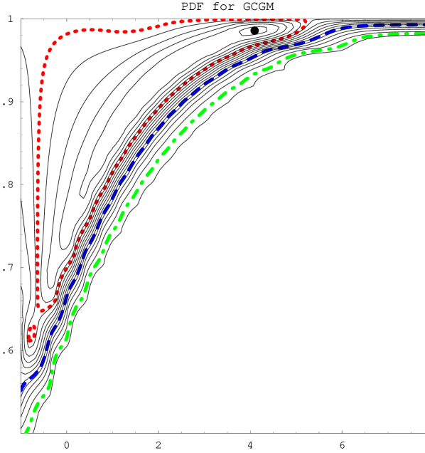
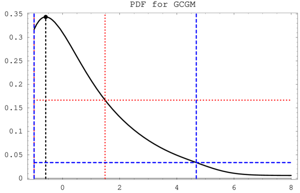
Note that the marginalized estimations differs substantially from those extracted from the minimization of $\chi^{2}$, which gives a large positive best value $\alpha$, but the dispersion is quite high, so even large positive values are not excluded, at least at $2\sigma$ level. And figure 2 for the joint probabilities for $\alpha$ and $\bar{A}$ and figures 3 and 4 for $\alpha$ and $\bar{A}$, respectively, clearly show that the marginalization process changes the peak values and credible regions depending on the number of dimensions.

Figure 2: The graphics of the joint PDF as function of $(\alpha,\bar{A})$ for the generalized Chaplygin gas model. The joint PDF peak is shown by the large dot, the credible regions of $1\,\sigma$ ($68,27\%$) by the red dotted line, the $2\,\sigma$ ($95,45\%$) in blue dashed line and the $3\,\sigma$ ($99,73\%$) in green dashed-dotted line. The cases for $\Omega_{m0}=0$ are not shown here because they are similar to the ones with $\Omega_{m0}=0.04$. The cases for $k=0$ are shown in figure $2$ of ref. [20].

Figure 3: The PDF of $\alpha$ for the generalized Chaplygin gas model. The solid lines are the PDF, the $1\sigma$ ($68.27\%$) regions are delimited by red dotted lines and the $2\sigma$ ($95.45\%$) credible regions are given by blue dashed lines. The cases for $\Omega_{m0}=0$ are not shown here because they are similar to the ones with $\Omega_{m0}=0.04$. The cases for $k=0$ are shown in figure $3$ of ref. [20].

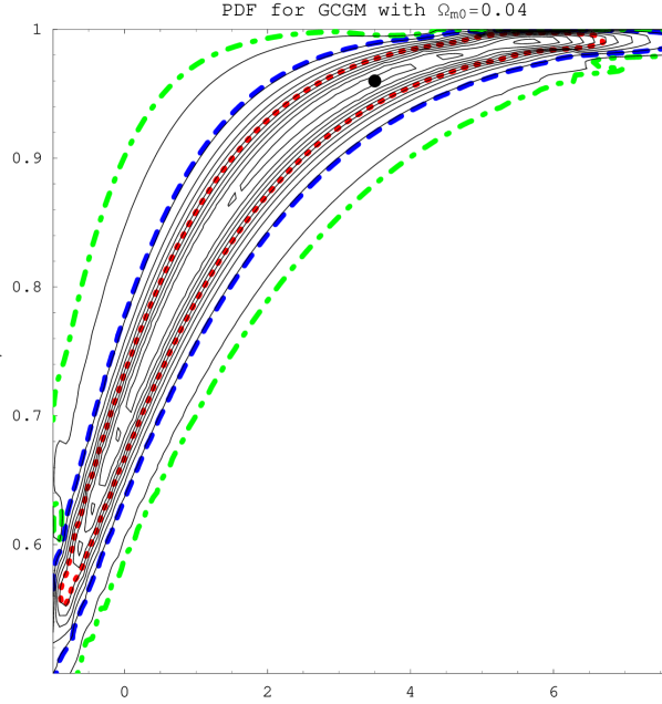
Of course, the CGM is obtained when $\alpha$ is fixed to unity. From the analysis of the GCGM it can be inferred that $p(\alpha=1)=40.81\%$, i.e., the CGM is favoured with a probability of $40.81\%$. Restricting to null curvature or fixing the pressureless matter density increases considerably this value, from $68.22\%$ to $91.09\%$. Analogously, the probability to have $\alpha>0$ (with more physical meaning) is $66.74\%$ and this value is quite increased when one or two parameters are fixed. Both $p(\alpha=1)$ and $p(\alpha>0)$ are increased with respect to ref. [20].

3.3 Estimation of $\bar{A}$

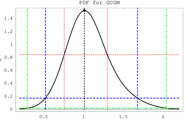
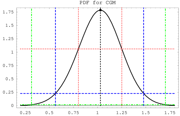
Like ref. [20], the results indicate that the value of $\bar{A}$ is close to unity, but now the dispersion is slightly smaller. In the case of GCGM with no fixed parameters, the marginalization of the remaining four other parameters leads to $\bar{A}=1.000_{-0.348}^{+0.000}$. Again, this could suggest the conclusion that $\Lambda$CDM ($\bar{A}=1$) model is favoured. However, the accuracy of the computation, due to the step (between $0.01$ and $0.02$) used in the evaluation of the parameter, does not allow this conclusion. Instead, it means the peak happens for $0.98<\bar{A}\leqslant 1$. In fact, fixing the curvature or the pressureless matter, the preferred value differs slightly from unity, for example the quartessence scenario, $\Omega_{m}=0$, yields $\bar{A}=0.987_{-0.3888}^{+0.012}$. But, differently from ref. [20], the CGM now predicts a best value for $\bar{A}$ smaller than unity, $\bar{A}=0.860_{-0.069}^{+0.140}$, and the best value becomes smaller when one or two parameters are fixed.

Figure 4: The one-dimensional PDF of $\bar{A}$ for the generalized and traditional Chaplygin gas model. The solid lines are the PDF, the $1\sigma$ ($68.27\%$) regions are delimited by red dotted lines, the $2\sigma$ ($95.45\%$) credible regions are given by blue dashed lines and the $3\sigma$ ($99.73\%$) regions are delimited by green dashed-dotted lines. The cases for $\Omega_{m0}=0$ are not shown here because they are similar to the ones with $\Omega_{m0}=0.04$. The cases for $k=0$ are shown in figures $4$ and $5$ of ref. [20].

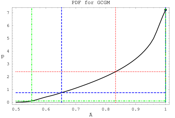
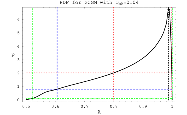
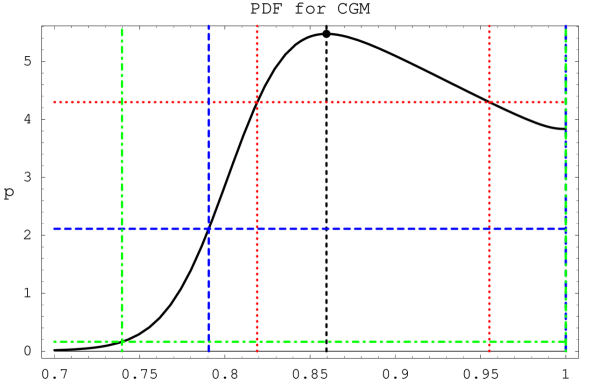
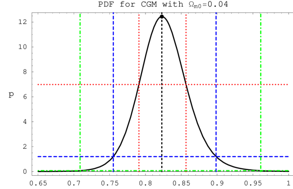
In figure 4 the PDF for $\bar{A}$ is displayed, both for the GCGM and the CGM, where the marginalization is made in all other parameters. Note that the probability to have $\bar{A}\neq 1$ (meaning how much the $\Lambda$CDM is rule out) is zero only for the GCGM (due to the step used in the evaluation of $\bar{A}$), but this probability varies from about $60\%$ to $100\%$ for other cases.

In figure 2 the joint probabilities for $\alpha$ and $\bar{A}$ are displayed, with a non-Gaussian shape. Comparing with ref. [20], the peak values now happen for large values of $\alpha$ and $\bar{A}$. This figure, compared to figures 3 and 4, is an illustration of the importance of the marginalization process because it changes the peak values and credible regions depending on whether two or one-dimensional parameter space is used.

3.4 Estimation of $\Omega_{m0}$ and $\Omega_{c0}$

Figure 5: The graphics of the joint PDF as function of $(\Omega_{m0},\Omega_{c0})$ for the generalized Chaplygin gas model, GCGM (traditional Chaplygin gas model, CGM), where $p(\Omega_{m0},\Omega_{c0})$ is a integral of $p(\alpha,H_{0},\Omega_{m0},\Omega_{c0},\bar{A})$ ($p(H_{0},\Omega_{m0},\Omega_{c0},\bar{A})$) over the $(\alpha,H_{0},\bar{A})$ ($(H_{0},\bar{A})$) parameter space. The joint normalized PDF peak has the value $4.624$ ($5.158$) for $(\Omega_{m0},\Omega_{c0})=(0.000,0.943)$ ($(\Omega_{m0},\Omega_{c0})=(0.000,1.099)$) shown by the large dot, the credible regions of $1\,\sigma$ ($68,27\%$, shown in red dotted line), $2\,\sigma$ ($95,45\%$, in blue dashed line) and $3\,\sigma$ ($99,73\%$, in green dashed-dotted line) have PDF levels of $1.577$, $0.345$ and $0.038$ ($2.191$, $0.439$ and $0.040$), respectively. As $\Omega_{k0}+\Omega_{m0}+\Omega_{c0}=1$, the probability for a spatially flat Universe is on the line $\Omega_{m0}+\Omega_{c0}=1$, above it we have the region for a closed Universe ($k>0$, $\Omega_{k0}<0$), and below, the region for an open Universe ($k<0$, $\Omega_{k0}>0$).

Figure 6: The graphics of the joint PDF as function of $(\Omega_{m0},\Omega_{c0})$ for the $\Lambda$CDM model model, where $p(\Omega_{m0},\Omega_{c0})$ is a integral of $p(H_{0},\Omega_{m0},\Omega_{c0})$ over the $H_{0}$ parameter space. The joint normalized PDF peak has the value $14.71$ for $(\Omega_{m0},\Omega_{c0})=(0.460,0.981)$ (shown by the large dot), the credible regions of $1\,\sigma$ ($68,27\%$, shown in red dotted line), $2\,\sigma$ ($95,45\%$, in blue dashed line) and $3\,\sigma$ ($99,73\%$, in green dashed-dotted line) have PDF levels of $4.634$, $0.675$ and $0.056$, respectively. As $\Omega_{k0}+\Omega_{m0}+\Omega_{c0}=1$, the probability for a spatially flat Universe is on the line $\Omega_{m0}+\Omega_{c0}=1$, above it we have the region for a closed Universe ($k>0$, $\Omega_{k0}<0$), and below, the region for an open Universe ($k<0$, $\Omega_{k0}>0$).

Figure 7: The one-dimensional PDF of $\Omega_{k0}$, $\Omega_{m0}$ and $\Omega_{c0}$ for the generalized Chaplygin gas model. The solid lines are the PDF, the $1\sigma$ ($68.27\%$) regions are delimited by red dotted lines, the $2\sigma$ ($95.45\%$) credible regions are given by blue dashed lines and the $3\sigma$ ($99.73\%$) regions are delimited by green dashed-dotted lines. The case for $\Omega_{m0}=0$ is not shown here because it is similar to the one with $\Omega_{m0}=0.04$. The case for $k=0$ is shown in figure $9$ of ref. [20]. As $\Omega_{c0}=1-\Omega_{k0}-\Omega_{k0}$, for $\Omega_{m0}=0$ we have $\Omega_{c0}=1-\Omega_{k0}$, for $\Omega_{m0}=0.04$ then $\Omega_{c0}=0.96-\Omega_{k0}$ and for $\Omega_{k0}=0$ we also have $\Omega_{c0}=1-\Omega_{m0}$.

Figure 8: The one-dimensional PDF of $\Omega_{k0}$, $\Omega_{m0}$ and $\Omega_{c0}$ for the traditional Chaplygin gas model. The solid lines are the PDF, the $1\sigma$ ($68.27\%$) regions are delimited by red dotted lines, the $2\sigma$ ($95.45\%$) credible regions are given by blue dashed lines and the $3\sigma$ ($99.73\%$) regions are delimited by green dashed-dotted lines. The case for $\Omega_{m0}=0$ is not shown here because it is similar to the one with $\Omega_{m0}=0.04$. The case for $k=0$ is shown in figure $10$ of ref. [20]. As $\Omega_{c0}=1-\Omega_{k0}-\Omega_{k0}$, for $\Omega_{m0}=0$ we have $\Omega_{c0}=1-\Omega_{k0}$, for $\Omega_{m0}=0.04$ then $\Omega_{c0}=0.96-\Omega_{k0}$ and for $\Omega_{k0}=0$ we also have $\Omega_{c0}=1-\Omega_{m0}$.

Figure 9: The one-dimensional PDF of $\Omega_{k0}$, $\Omega_{m0}$ and $\Omega_{c0}$ for the $\Lambda$CDM model. The solid lines are the PDF, the $1\sigma$ ($68.27\%$) regions are delimited by red dotted lines, the $2\sigma$ ($95.45\%$) credible regions are given by blue dashed lines and the $3\sigma$ ($99.73\%$) regions are delimited by green dashed-dotted lines. The case for $\Omega_{m0}=0$ is not shown here because it is similar to the one with $\Omega_{m0}=0.04$. The case for $k=0$ is shown in figure $11$ of ref. [20]. As $\Omega_{c0}=1-\Omega_{k0}-\Omega_{k0}$, for $\Omega_{m0}=0$ we have $\Omega_{c0}=1-\Omega_{k0}$, for $\Omega_{m0}=0.04$ then $\Omega_{c0}=0.96-\Omega_{k0}$ and for $\Omega_{k0}=0$ we also have $\Omega_{c0}=1-\Omega_{m0}$.

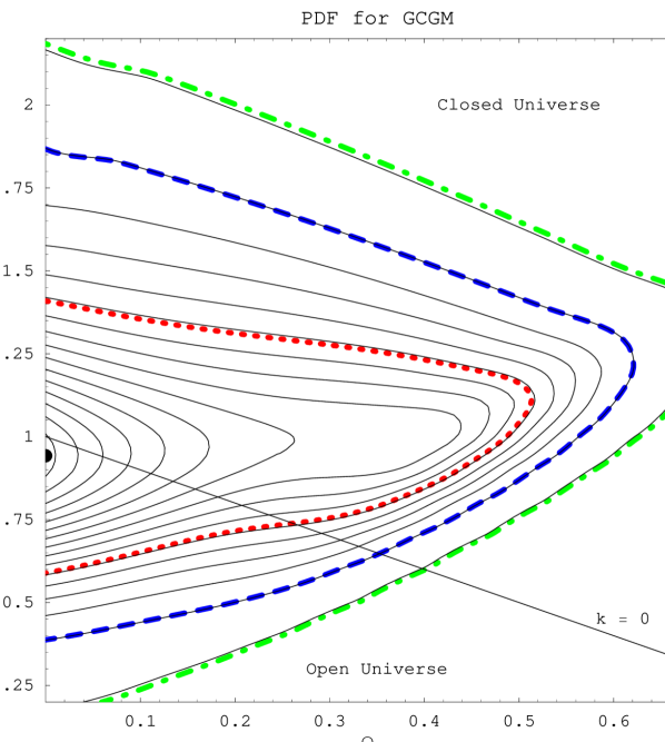
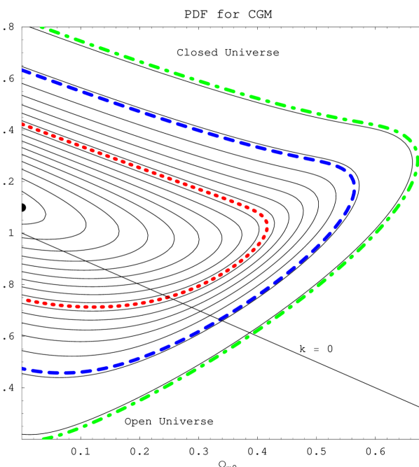
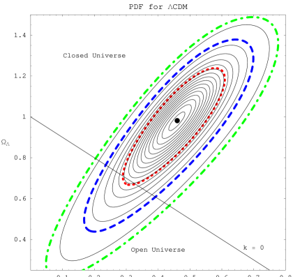
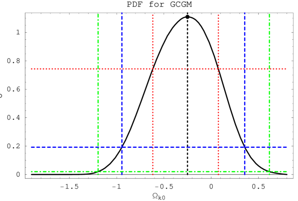
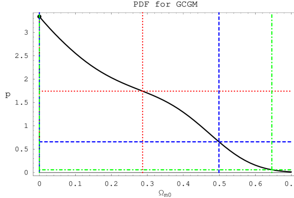
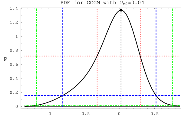
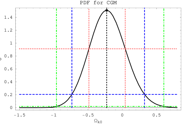
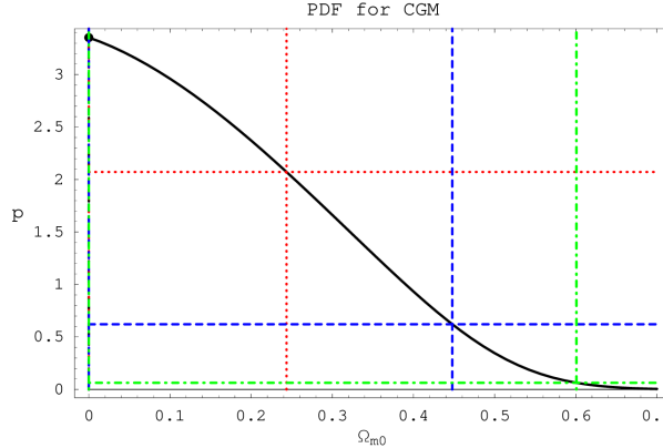
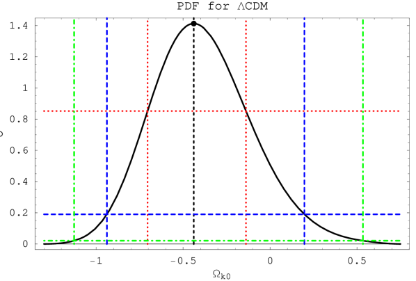
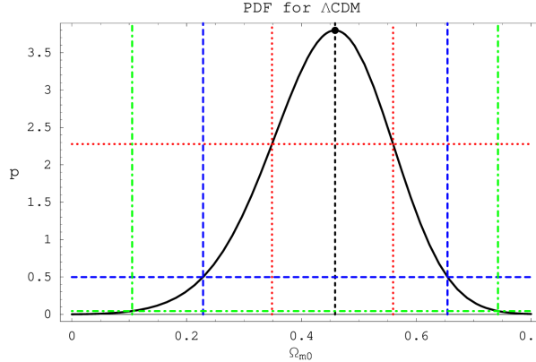
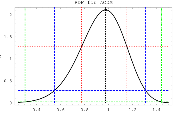
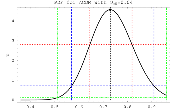
The unified scenario of quartessence, with no pressureless matter, is again favoured as, for example, the GCGM and CGM (without fixed parameters) predict $\Omega_{m0}=0.000_{-0.000}^{+0.499}$ and $\Omega_{m0}=0.000_{-0.000}^{+0.448}$, respectively. The same estimations from ref. [22], $\Omega_{m0}=0.00_{-0.00}^{+0.86}$, and ref. [21], $\Omega_{m0}=0.00_{-0.00}^{+0.82}$, show that the increased number of SNe Ia has substantially decreased the estimated error. Compared to ref. [20], the dispersion is also highly decreased, which once more favours the quartessence scenario. The case of flat Universe has an even smaller dispersion for the quartessence model. See figures 7 and 8.

Like ref. [20], the GCGM, the CGM and the $\Lambda$CDM remarkably lead to almost the same predictions concerning the dark energy component, $\Omega_{c0}$, when all parameters are free: $1.012^{+0.667}_{-0.489}$, $1.030^{+0.448}_{-0.467}$ and $0.976^{+0.333}_{-0.426}$, respectively. By comparing with ref. [20], now $\Omega_{c0}$ (which behaves as $\Omega_{\Lambda}$ for $\Lambda$CDM) has lower values and narrower dispersions, like $\Omega_{m0}$, see figures 7–9.

The joint probability for $\Omega_{m0}$ and $\Omega_{c0}$ is now smoother for the GCGM and the CGM cases (figure 5), with the $1\sigma$, $2\sigma$ and $3\sigma$ contours of figures 5 and 6 showing significantly smaller regions. So the analysis for $\Lambda$CDM is now quite in agreement with the results of ref. [26].

3.5 Estimation of $\Omega_{k0}$

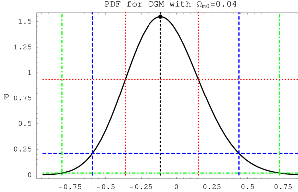
In comparison with ref. [20], a closed Universe is still clearly favoured, but with slightly smaller probability, i.e., $p(\Omega_{k0}<0)$. But more important, the dispersion for $\Omega_{k0}$ is now substantially narrowed, as shown by figures 7–9. The probability to have a flat Universe, $p(\Omega_{k0}=0)$, is now greater ($45.70\,\%$, $39.84\,\%$ and $15.44\,\%$ for GCGM, CGM and $\Lambda$CDM), and after setting the pressureless matter it increases, exception being the $\Lambda$CDM case.

With respect to refs. [21, 22] (using the selected 26 SNe Ia data), the dispersion has also significantly decreased, for example : $\Omega_{k0}=-0.251_{-0.694}^{+0.605}$ and $\Omega_{k0}=-0.228_{-0.508}^{+0.552}$ versus $\Omega_{k0}=-0.74_{-1.32}^{+1.42}$ [22] and $\Omega_{k0}=-0.84_{-1.23}^{+1.51}$ [21], for respectively GCGM and CGM.

3.6 Estimation of the age of the Universe, $t_{0}$

Due to the larger number of SNe Ia used here with respect to refs. [21, 22], the dispersions have been quite decreased. For example, $t_{0}=14.42_{-1.77}^{+2.51}\,Gy$ and $t_{0}=13.93_{-0.65}^{+0.97}\,Gy$ estimated here for the GCGM and CGM versus $t_{0}=15.3^{+4.2}_{-3.2}\,Gy$ [22] and $t_{0}=14.2^{+2.8}_{-1.5}\,Gy$ [21], respectively.

The predicted age of the Universe when no parameter is fixed has increased with respect to ref. [20], fortunately not anymore dangerously near the recent estimations age of the globular clusters [32], $t_{0}=12.6^{+3.4}_{-2.4}\,Gy$.

3.7 Estimation of the deceleration parameter $q_{0}$

The values for the deceleration parameter $q_{0}$ are increased (less negative) with respect to ref. [20]. The estimated errors are significantly smaller than the ones of refs. [21, 22], for example : $q_{0}=-0.730_{-0.328}^{+0.352}$ and $q_{0}=-0.769_{-0.309}^{+0.358}$ versus $q_{0}=0.80_{-0.62}^{+0.86}$ [22] and $q_{0}=0.98_{-0.62}^{+1.02}$ [21], for respectively GCGM and CGM.

In all cases, $p(q_{0}<0)$, the probability to have an accelerating Universe today, is equal to or very near $100\%$.

3.8 Estimation of the scale factor $a_{i}$ the Universe begins to accelerate from

Another useful quantity is the scale factor at the moment the Universe begins to accelerate, $a_{i}$, keeping in mind that the scale factor is normalized with its present value $a_{0}$ equal to unity. With respect to ref. [20], $a_{i}$ decreases when no parameter is fixed. As expected, the larger number of supernovae in comparison with ref. [22] yields smaller credible intervals for $a_{i}$, for example $a_{i}=0.626_{-0.123}^{+0.184}\,a_{0}$ estimated here for GCGM versus $a_{i}=0.67_{-0.37}^{+0.25}\,a_{0}$ of ref. [22].

The probability the Universe begins to accelerate before today, $p(a_{i}<1)$ in tables 6– 11, is essentially $100\%$, being approximately the same value of the probability to have an accelerating Universe today, i.e., $p(q_{0}<0)$. Theoretically they should be the same, so the fact that these independent probability calculations agree almost exactly shows the accuracy and reliability of the Bayesian probability analyses of this work.

4 Conclusions

The present work has performed the most extensive analysis of  the GCGM and CGM in what concerns the comparison of theoretical predictions with the type Ia supernovae data, using the 157 data of the “gold sample”. By using the high productivity of BETOCS (BayEsian Tools for Observational Cosmology using SNe Ia [23]), it was possible to make all the best-fittings, parameter estimations and figures shown here.

All positive features of GCGM and CGM were enhanced with respect to ref. [20] :

• the probability to have $\alpha>0$ (with more physical meaning) is increased, as well as both $p(\alpha=1)$ and $p(\alpha>0)$;

• value of $\bar{A}$ now has slightly smaller dispersion;

• the dispersion of $\Omega_{m0}$ and $\Omega_{c0}$ are also highly decreased, favouring even more the quartessence [13, 27] scenario;

• the dispersion for $\Omega_{k0}$ is now substantially narrowed, and the probability to have a flat Universe is now greater;

• predicted age of the Universe (when no parameter is fixed) has increased, fortunately not anymore dangerously near the recent estimations age of the globular clusters.

One important result concerns the Hubble parameter, $H_{0}$. It is not acceptable to fix its value because arbitrary parameter estimations and usually bad best-fittings are obtained. As the HST (Hubble Space Telescope) prior [25] for $H_{0}$ implies minor effects on all results, we can choose a flat or HST prior.

The CGM (traditional Chaplygin gas model), where $\alpha=1$, remains competitive and preferred in many cases : when the five parameters are considered, the probability is $40.81\%$, but increases as much as to $95.94\%$ for the quartessence scenario.

For the parameter $\bar{A}$, both GCGM and CGM cases of fixed curvature and matter densities shows a value near but small than $1$ as the best value of $\bar{A}$, such that the $\Lambda$CDM case ($\bar{A}=1$) is almost ruled out.

The results indicate that, for the GCGM, CGM and $\Lambda$CDM, a closed Universe is favoured. The GCGM and CGM favour the unified scenario (quartessence), where the pressureless matter density is essentially zero.

There are many current and future applications [20, 21, 22, 33] and developments of BETOCS : using different SNe Ia data sets (SNLS [34], etc), different priors, different cosmological models [35], etc. We plan to release variant versions for other observational cosmological data [36, 37, 38, 39], like BETOCX (BayEsian Tools for Observational Cosmology using X-ray gas mass fraction of galaxy clusters), so it will be possible to cross the estimations from different observational data.

Acknowledgments

The authors are also grateful by the received financial support during this work, from FACITEC/PMV (R. C. Jr.) and CNPq (R. G.).

References

- [1] A. Riess et al, Astron. J. 116, 1009 (1998);
- [2] S. Perlmutter et al, Astrophys. J. 517, 565 (1999);
- [3] D. N. Spergel et al, Astrophys. J. Suppl. 148, 175 (2003);
- [4] E. L. Turner, J. P. Ostriker, and J. R. Gott III, Astrophys. J. 284, 1 (1984).
- [5] M. Fukugita, T. Futamase, and M. Kasai, Mont. Not. R. Astron. Soc. 246, 24 (1990).
- [6] S.W. Allen et al., Monthly Notices of the Royal Astron. Society 353, 457 (2004);
- [7] Bagla J. S., Padmanabhan T., Narlikar J. V., 1996, Comments on Astrophysics 18, 275; astro-ph/9511102;
- [8] S. Weinberg, Rev. Mod. Phys. 61, 1 (1989);
- [9] S. M. Carroll, Living Rev. Rel. 4, 1 (2001);
- [10] R. R. Caldwell, R. Dave and P. J. Steinhardt, Phys. Rev. Lett. 80, 1582 (1998);
- [11] I. Zlatev, L. Wang and P. J. Steinhardt, Phys. Rev. Lett. 82, 896 (1999);
- [12] A. Kamenshchik, U. Moschella, and V. Pasquier, Phys. Lett. B 511, 265 (2001);
- [13] M. Makler, Gravitational Dynamics of Structure Formation in the Universe, PhD Thesis, Brazilian Center for Research in Physics (2001);
- [14] N. Bilić, G.B. Tupper, and R.D. Viollier, Phys. Lett. B 535, 17 (2002);
- [15] M.C. Bento, O. Bertolami, and A.A. Sen, Phys. Rev. D 66, 043507 (2002);
- [16] R. Jackiw, A particle field theorist’s lectures on supersymmetric, non-abelian fluid mechanics and d-branes, physics/0010042;
- [17] J. C. Fabris, S. V. B. Gonçalves and P. E. de Souza, Gen. Rel. Grav. 34, 53 (2002);
- [18] H. Sandvik, M. Tegmark, M. Zaldarriaga e I. Waga, Phys. Rev. D69, 123524 (2004);
- [19] L. M. G. Beça, P. P. Avelino, J. P. M. de Carvalho and C. J. A. P. Martins, Phys. Rev. D67, 101301 (2003);
- [20] R. Colistete Jr., J. C. Fabris, Class. Quantum Grav. 22, 2813 (2005);
- [21] R. Colistete Jr., J. C. Fabris, S. V. B. Gonçalves and P. E. de Souza, Int. J. Mod. Phys. D13, 669 (2004);
- [22] R. Colistete Jr., J. C. Fabris and S. V. B. Gonçalves, Int. J. Mod. Phys. D14, 775 (2005);
- [23] R. Colistete Jr., BayEsian Tools for Observational Cosmology using SNe (BETOCS), available on the Internet site http://www.RobertoColistete.net/BETOCS, (2006);
- [24] S. Wolfram, The Mathematica Book (Cambridge University Press), 1999.
- [25] W. Freedman, Astrophys. J. 553, 47 (2001).
- [26] A. G. Riess et al, Astrophys. J. 607, 665 (2004);
- [27] M. Makler, S. Q. Oliveira, and I. Waga, Phys. Lett. B, 555, 1 (2003).
- [28] T. J. Loredo, in ‘Maximum Entropy and Bayesian Methods’, ed. P.F. Fougere, Kluwer Academic Publishers, Dordrecht (1990) ;
- [29] T. J. Loredo, in ‘Statistical Challenges in Modern Astronomy’, ed. E.D. Feigelson and G.J. Babu, Springer-Verlag, New York (1992);
- [30] P. C. Gregory and T.J. Loredo, Astrophys. J. 398, 146 (1992);
- [31] M. E. Abroe et al., Mon. Not. R. A. Soc. 334, 11 (2002);
- [32] L.M. Krauss, The state of the Universe: cosmological parameters 2002, astro-ph/0301012;
- [33] F. Casarejos, J. C. Fabris, S. V. B. Gonçalves and J. F. Villas da Rocha, Constraining double component dark energy model using type Ia supernovae data, astro-ph/0606171;
- [34] P. Astier et al. (SNLS colaboration), Astron. Astrophys. 447, 31 (2006);
- [35] S. Nesseris and L. Perivolaropoulos, Phys. Rev. D 70, 043531, (2004);
- [36] H. K. Jassal, J. S. Bagla and T. Padmanabhan, The vanishing phantom menace, astro-ph/0601389;
- [37] S. Nesseris and L. Perivolaropoulos, Crossing the Phantom Divide: Theoretical Implications and Observational Status, astro-ph/0610092;
- [38] J. V. Cunha, J. S. Alcaniz and J. A. S. Lima, Phys. Rev. D69, 083501 (2004);
- [39] L. Amendola, M. Makler, R. R. R. Reis and I. Waga, Phys. Rev. D 74, 063524 (2006).