A limit on the presence of Earth-mass planets around a Sun-like star

Abstract

We present a combined analysis of all publicly available, visible HST observations of transits of the planet HD 209458b. We derive the times of transit, planet radius, inclination, period, and ephemeris. The transit times are then used to constrain the existence of secondary planets in the system. We show that planets near an Earth mass can be ruled out in low-order mean-motion resonance, while planets less than an Earth mass are ruled out in interior, 2:1 resonance. We also present a combined analysis of the transit times and 68 high precision radial velocity measurements of the system. These results are compared to theoretical predictions for the constraints that can be placed on secondary planets.

1 Introduction

The discovery of 51 Peg B (Mayor & Queloz, 1995) fulfilled a many-decade quest to discover extrasolar planets around main sequence stars. The discovery of the first transiting planet HD 209458b (Charbonneau et al., 2000; Henry et al., 2000) allowed the confirmation that radial velocity variations were indeed due to planets and not some other period stellar phenomenon. Currently ten transiting planets have been found, allowing a measurement of the mass-radius relation for short period extrasolar planets (Charbonneau et al., 2006). Besides confirming that radial velocity variations are due to real objects with the sizes and masses of planets, transiting planets have allowed a host of other questions to be addressed, for example, the planet atmospheric composition (Charbonneau et al., 2002), constraints on the presence of planetary satellites (Brown et al., 2001), detection of thermal emission from the planets (Deming et al., 2005; Charbonneau et al., 2005), and the size of the planet core as a function of stellar metallicity (Guillot et al., 2006).

In this paper we provide another application of transiting planetary systems: we place a constraint on the presence of terrestrial-mass planet companions in mean-motion resonance with HD 209458b. As shown in Agol et al. (2005), a planet in resonance induces a libration of the transiting planet with an amplitude $\sim 0.2j^{-1}(M_{2}/M_{1})P_{1}$, where $M_{1},P_{1}$ are the mass and period of the known transiting planet and $M_{2}$ is the mass of the companion planet in a $j$:$j+1$ resonance. For HD 209458b, this translates into a variation in the times of transit with a 3 minute amplitude and few month period for $M_{2}=m_{\oplus}$. Since this technique relies on a precise measurement of the times of transit, we use the highest precision photometry available for thirteen transits measured by the Hubble Space Telescope (Brown et al., 2001; Schultz et al., 2004; Knutson et al., 2006). We carry out an analysis of the transit times with a careful quantifying of the timing errors (§2). We use these results to constrain the transiting planet parameters (§3). We then use these derived times of transit to place a constraint on a secondary coplanar planet (§4). We finish up with a comparison of these results with those derived for the TrES-1 transiting planet system (§4.1) and a comparison with the constraints from radial-velocity measurements (§4.2).

2 Data Analysis

At least ten science observing programs with the Hubble Space Telescope have proposed to observe transits of the planet in the HD 209458 system. The five ultraviolet observations do not have enough photons to measure the transit lightcurve precisely, while four programs have made observations of the planetary transit in the optical, of which three are now publicly available: 8789, 9171 and 9447 (the other program, 10145, has not been fully made public yet). Two programs, Brown 8789 and Charbonneau 9447, utilized the STIS spectrograph as a CCD photometer. By spreading the light from the star with a grism, in an effort to capture as many photons as possible, their relative photometry is likely the most precise ever obtained (Brown et al., 2001; Knutson et al., 2006). The third program utilized the Fine Guidance Sensors to carry out rapid high precision photometry (Schultz et al., 2004). These programs give a total of thirteen transits observed with HST. The primary motivation for these observations was to constrain the planetary parameters, to detect absorption features in the planet’s atmosphere, and to search for satellites of the planet. However, these data are also useful for timing each transit to measure a precise ephemeris (Wittenmyer et al., 2005) and to look for deviations from exact periodicity. A summary of the observations is given in table 1.

Table 1: Overview of the HST observations of the HD 209458 system including the instrument, wavelength range, cadence, and date of observation.

Transit	Transit number	Orbits	Instrument	Filter/Grating	wavelength range	exposure/readout time	date
1	0	5	STIS	G750M	581.3-638.2 nm	60/20 sec	UT 2000 April 25
2	1	5	STIS	G750M	581.3-638.2 nm	60/20 sec	UT 2000 April 28-29
3	3	5	STIS	G750M	581.3-638.2 nm	60/20 sec	UT 2000 May 5-6
4	5	5	STIS	G750M	581.3-638.2 nm	60/20 sec	UT 2000 May 12-13
5	117	3	FGS	F550W	510-587.5 nm	0.025/0 sec	UT 2001 Jun 11
6	143	2	FGS	F550W	510-587.5 nm	0.025/0 sec	UT 2001 Sep 11
7	160	2	FGS	F550W	510-587.5 nm	0.025/0 sec	UT 2001 Nov 10
8	179	2	FGS	F550W	510-587.5 nm	0.025/0 sec	UT 2002 Jan 16
9	252	2	FGS	F550W	510-587.5 nm	0.025/0 sec	UT 2002 Sep 30
10	313	5	STIS	G430L	290-570 nm	22/20 sec	UT 2003 May 3
11	321	5	STIS	G750L	524-1027 nm	19/20 sec	UT 2003 May 31
12	328	5	STIS	G430L	290-570 nm	22/20 sec	UT 2003 Jun 25
13	331	5	STIS	G750L	524-1027 nm	19/20 sec	UT 2003 Jul 5-6

2.1 Reduction of pipeline data

We re-reduced these data from the pipeline calibrated products that are available in the archive. We followed the reduction procedures described in Brown et al. (2001) and Schultz et al. (2004), but summarize the most important steps for each data set here. For the STIS data we carried out the minimum reduction necessary to obtain precise photometry. We subtracted cosmic rays using a 5 sigma rejection of the time series for each pixel within an HST orbit, we binned the photons within 8 pixels of the spectrum peak (17 pixels wide) to derive the total counts for each frame, and assigned the midpoint of each exposure as the time for each frame. We discarded the first frame from each orbit. For the first transit observed in program 8789 we only used the data for which the spectrum centroid was greater than 4 pixels from the edge of the CCD (see discussion in Brown et al., 2001) and we did not utilize the first and last columns of the CCD which show larger errors. The 1-sigma errors on the flux are taken from the pipeline calibrated errors which are summed in quadrature. For the FGS data we took the sum of the four photometers, discarded data which deviated more than 3 sigma from a fourth order fit to the time series for each orbit, and binned the data to 80 second bins (10 second bins gave the same results) with the time stamp at the center of each bin. With these time series we then fit a model for the transiting planet and the flux sensitivity variations of Hubble, which we describe next.

2.2 Photometric Error bars

The errors computed from the pipeline include counting noise and, for the CCD data, read noise. We examined the scatter in the data compared to the computed error bars and found that the scatter was larger than the pipeline errors for the FGS data and second set of STIS data. This could not be attributed solely to cosmic rays and we were not able to identify the additional error source. Consequently, we estimated the errors for each transit individually by analyzing the out-of-transit data.

To account for the fluctuations in sensitivity of HST when we determine the size of the error bars, we fit a model to the out-of-transit data for each transit with two components: i) an $n$th order polynomial fit as a function of the orbital phase of HST ii) a linear fit as a function of time. We measured the standard deviation of the residuals of this fit in units of the statistical error of each point as a function of $n$, and measured the median of this standard deviation for all thirteen transits as a function of $n$. We found that between $n=5$ and $n=6$ the median of the standard deviation ratio was constant, indicating that including a 6th order term did not significantly improve the fit to the fluctuations in sensitivity as a function of the HST orbital phase. The residuals did not correlate with the HST orbital phase, so we then assigned the greater of the standard deviation of the residuals for $n=5$ or the statistical error. The first five transits (Table 1) had statistical errors nearly equal to the residuals, while the error bars of the remaining transits were increased by 20-50%. These changes to the error bars were used throughout the remainder of the analysis.

2.3 Planet orbit and transit model

We model the lightcurves by treating the planet and star as perfectly spherical, and by assuming that the planet is on a circular orbit (Laughlin et al., 2005; Deming et al., 2005). Thus, there are only three free parameters to describe the planet’s orbit: the ratio of the planet to star radius, $R_{p}/R_{s}$; the ratio of the relative velocity of the planet and star to the stellar radius, $v/R_{s}$; and the inclination of the planet’s orbit, $i$. In addition, we allowed the time of each transit to be a free parameter, giving thirteen transit times. From these is derived the period of the planet, $P$, which then gives the ratio of the semi-major axis to the stellar radius, $a/R_{s}=(v/R_{s})P/(2\pi)$, necessary for computing the relative position of the planet and star. In this approach the actual values of the planet and stellar radii cannot be determined, only their relative values (to determine the absolute values requires fitting the radial velocities and using a stellar mass-radius relation as in Cody & Sasselov, 2002; Knutson et al., 2006).

2.4 Limb darkening

If the lightcurves for each transit were only affected by Poisson noise and were continuously sampled, then assumptions about the shape of the transit lightcurve would be unnecessary: the mid-point of transit could be found by simply assuming the transit lightcurve was symmetric about mid-transit. However, the HST data are affected by sensitivity variations due to temperature changes in the telescope and by observing gaps, both due to Earth occultation. This fact forces us to choose a model for the transit lightcurve in order to solve for the transit time, i.e. time at transit midpoint. The primary uncertainty in the modeling is the shape of the stellar limb darkening. To test the robustness of the transit times to assumptions about limb-darkening, we modeled the limb-darkening of the star with two approaches: stellar atmosphere predictions and quadratic limb-darkening.

In the first case we used the computed limb-darkening from Phoenix NextGen stellar atmosphere models (Claret & Hauschildt, 2003). These models include an accurate, high-resolution treatment of the brightness at the limb using spherically-symmetric stellar models. We used an atmosphere of 6100 K and a surface gravity of $log(g)=4.5$, appropriate for HD 209458a (Valenti & Fischer, 2005). We convolved the wavelength-dependent limb-darkening with the number of photons detected at each wavelength (for the FGS we convolved the FGS sensitivity with a stellar atmosphere to estimate the relative number of photons detected as a function of wavelength). The resulting limb darkening is shown in Figure 1. There is only a gradual change in the limb darkening between the four different instrument/filter combinations, but given the timing precision required, these differences are significant. We then used a cubic spline interpolation of the limb darkening to integrate over the portion of the stellar disk occulted by the planet. The result is a more gradual ingress and egress than that predicted by analytic limb-darkening models which have a sharp edge.

Figure 1: Limb darkening for the four instrumental configurations - the vertical axis is the surface brightness of the star, $I$, as a function of $\mu=\cos{\theta}$, where $\theta$ is the polar angle measured from the line of sight to the star. Solid line is for STIS G750M, dotted line is for FGS F550W, dashed line is for STIS G430L, while dash-dot line is for STIS 750L.

In the second case we assumed that the limb-darkening was a quadratic function in the cosine of the polar angle measured from the line of sight. We utilized the routines from Mandel & Agol (2002) for computation of the lightcurves (this led to eight free parameters for the four filter/instruments combinations used in the data). We primarily used this case to check that the timing results are insensitive to the accuracy of the limb-darkening predicted from the atmosphere model, discussed more below.

2.5 HST flux sensitivity variations

Thermal fluctuations during the orbit of HST lead to changes in the sensitivity of each instrument at the 0.5% level. Fortunately these variations appear to be fairly reproducible during successive orbits (in addition to a smaller linear drift between successive orbits), but they are not reproducible on longer timescales. Following Brown et al. (2001) and Schultz et al. (2004) we phased the observations of each transit to the HST orbital period ($p_{h}$). We used two models for the variation of the flux sensitivity with orbital phase and two models for the “secular” variation with time over each transit, combined together giving a total of four models for the background variations. The orbital phase variation we modeled as i) a fifth-order polynomial, $\sum_{i=0}^{4}c_{i}\phi^{(i+1)}$, where $0\leq\phi<2\pi$ is the orbital phase of Hubble, or ii) as a linear and two harmonic functions of orbital phase, $c_{0}\phi+c_{1}\sin(\phi)+c_{2}\cos(\phi)+c_{3}\sin(2\phi)+c_{4}\cos(2\phi)$. The secular variation with time we modeled either as a linear function, $c_{5}f_{tran}(t)+c_{6}t$, where $f_{tran}$ is the transit lightcurve model normalized to unity outside transit, or a constant coefficient for each HST orbit, $c_{i+5}f_{tran,i}(t)$ where $i$ labels each HST orbit. The lightcurve model depends on sixteen non-linear parameters (the 3 planetary orbital parameters and 13 transit times). For the models of the HST flux sensitivity variations there are either $7\times 13=91$ or $5\times 13+51=116$ linear parameters. Coincidentally, the physically interesting parameters are non-linear, while the uninteresting parameters are linear.

To most efficiently find the best-fit for all 107 or 132 parameters, we used the following procedure:

1) We carried out a minimization over the 16 non-linear parameters using the MINPACK non-linear least squares routine (Cowell, 1984).

2) The model lightcurve for each transit we computed by carrying out a linear least-squares fit for the 91 or 116 linear parameters.

This procedure converged rapidly to the best $\chi^{2}$. We mapped the $\chi^{2}$ as a function of each non-linear parameter (while marginalizing over the other parameters), finding that the $\chi^{2}$ has a quadratic shape near the minimum, indicating that there is a unique solution.

2.6 Timing Error computation

The best-fit models have reduced chi-square in the range $\bar{\chi}^{2}=1.07-1.25$ for the four different flux sensitivity models. The reduced chi-squares for the FGS data (which contain fewer data points) were as high as 2.6 (for the 5th transit) indicating that the models were a poor fit to the data. We examined the residuals of the FGS data and found that some residuals within the transits were correlated. Thus our best fitting models were not a sufficiently good description of the data (either due to errors in the limb darkening or inaccuracies of the modeling of the HST flux sensitivity variations). Therefore, to obtain a better estimate of the error bars, taking into account these systematic effects, we used a Monte Carlo bootstrap simulation of the errors in which we shifted the residuals by a random number of points for each transit so that the correlations were maintained. We also reversed the residuals for each orbit and repeated the shift. We followed this procedure 200 times, added the shifted residuals to the best-fit model, and then re-fit using the same procedure that was applied to the original data described in the previous section. Our expectation is that this procedure gives an estimate of the errors due to inaccuracies in our assumed flux sensitivity models. We found that the resulting errors on non-linear model parameters, such as transit times, were larger by a factor of a few than if we simply used Poisson errors for the bootstrap or resampled the residuals randomly.

Although this process gives an indication of the size of the systematic errors, we also assessed the systematic errors by comparing the results from the four different HST flux sensitivity variation models. The differences in $\chi^{2}$ between the four different models was small - all had reduced $\chi^{2}$ near unity, so it is difficult to favor one particular sensitivity variation model. However, the differences between the derived transit times for each model was larger than the size of the error bars for a given model. We believe that this discrepancy is probably due to imperfections in all of the four flux sensitivity models, so we have taken the mean and standard deviations of all eight hundred Monte-Carlo simulations as an estimate of the transit times and their errors. Finally, to check the robustness of the stellar atmosphere limb-darkening we have used the quadratic limb-darkening law with the polynomial function of phase and linear secular term to fit the transit times. We find that these times agree within the errors with the times derived using the stellar atmosphere model and the same flux sensitivity model, so we conclude that the stellar atmosphere limb-darkening model provides an accurate estimate of the transit times of the data.

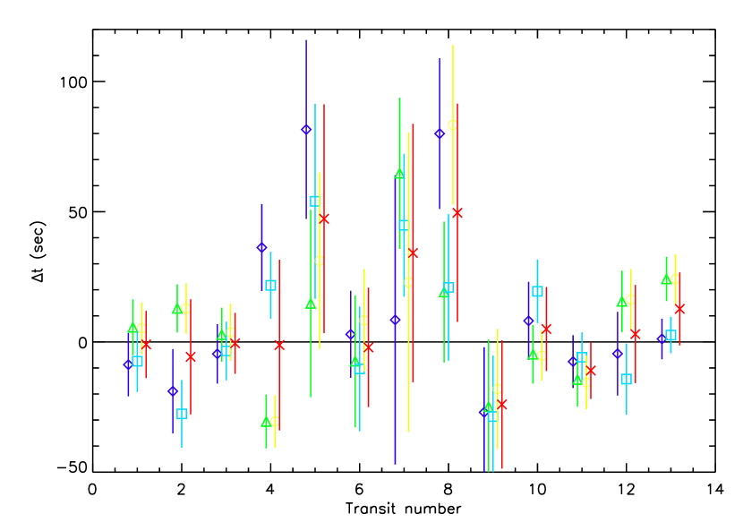
To these measured transit times we apply a correction for the motion of the Earth about the barycenter of the solar system (a heliocentric correction is insufficient as it differs from barycentric by up to 5 seconds). The motion of the Hubble Space Telescope about the Earth contributes a negligible timing error. The resulting transit times are reported in Table 2. We find from the Monte Carlo simulations that there is no significant correlation between the individual transit times so we report the standard deviation of each time without the full covariance matrix. Our fitted transit times agree well with those obtained by (Knutson et al., 2006), most being within 1/2 $\sigma$. The largest discrepancies are for transits 12 and 13 which disagree by 1.25 $\sigma$ and 0.75 $\sigma$ respectively. In the analysis by Knutson et al. (2006) it is these same transits which deviate most significantly from a constant period.

Table 2: Transit time and uncertainty in days and in seconds for the 13 observed transits.

Transit	Transit time	Error	Error
	(- 2450000 BJD)	(days)	(seconds)
1	1659.93678	0.00015	12
2	1663.46150	0.00025	21
3	1670.51102	0.00013	11
4	1677.56044	0.00037	31
5	2072.33284	0.00049	42
6	2163.97574	0.00028	24
7	2223.89685	0.00058	50
8	2290.86741	0.00051	44
9	2548.17311	0.00029	24
10	2763.18306	0.00018	15
11	2791.38087	0.00013	10
12	2816.05431	0.00021	18
13	2826.62867	0.00017	14

Figure 2: Differences of transit times from uniform period versus number of transit (each point is shifted horizontally slightly for clarity). Green/triangle- polynomial and linear; yellow/circle - harmonic and linear; dark blue/diamond - polynomial and flux offset for each orbit; light blue/square - harmonic and flux offset for each orbit. Red/cross points are mean and standard deviation of all four flux sensitivity models.

3 Results

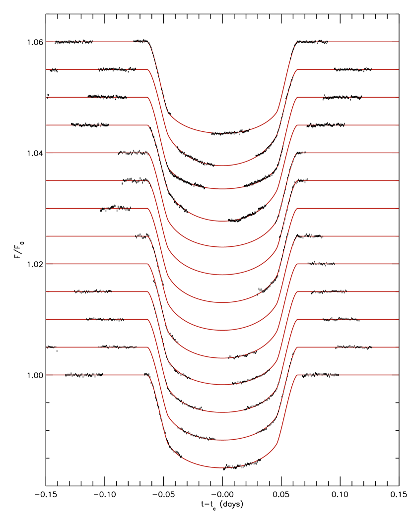
The results of the best fit models are shown in Figure 3.

Figure 3: Best-fit models overplotted with data (some data -0.15 days before mid-transit is off the plot). The data points are plotted with error bars, while the best-fit model is plotted as a red line. Each transit has been normalized to one out of transit and shifted by 0.05; the bottom is transit 1 and the top is transit 13.

3.1 Constraints on radius, inclination

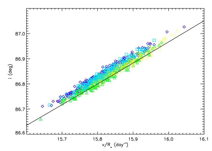
Since the data consist of a time series, the best constrained parameters are the period, $P$, and the duration of each transit, $T_{t}$. This leads to a degeneracy between the physical parameters: inclination and velocity. The relation between velocity and inclination is given by

$$v=R_{*}\left({T_{t}^{2}\over 4}+{P^{2}\over 4\pi^{2}}\cos^{2}{i}\right)^{-1/2}.$$ (1)

As long as $v$ and $i$ obey this relation, $P$ and $T_{t}$ are unchanged. Thus, for a very small uncertainty in $T_{t}$ and $P$, there can be a larger uncertainty in $i$ and $v/R_{*}$. The inclination is constrained by the shape of the limb-darkening and the duration of ingress and egress, which partially (but not completely) break the velocity-inclination degeneracy. In Figure 4 we show the results of our fitting for $\hat{v}=v/R_{*}$ and $i$. We plot the results of Monte Carlo simulations of each of the four models discussed above. The correlation between velocity and inclination follows equation 1 as expected.

We derive a radius of $R_{p}/R_{*}=0.1201\pm 0.0006$, consistent at 1$\sigma$ with the radius derived in Mandel & Agol (2002) (our derived error is larger since we have taken into account correlated photometric errors using the Monte Carlo analysis). We derive a velocity of $v/R_{*}=15.835\pm 0.065$ days^-1, which combined with the period gives the ratio of the size of the semi-major axis to the size of the star, $a/R_{*}=8.883\pm.036$. We derive an inclination of $i=1.5157\pm 0.00095$ or $i=86.845^{\circ}\pm 0.055^{\circ}$ which is consistent with that reported in Brown et al. (2001), although our derived error bar is smaller due to our using a fixed limb-darkening law. Since one can only derive dimensionless parameters or parameters with dimensions of time or flux directly from the lightcurve, we cannot measure the absolute size of the star, orbit, or planet.

Figure 4: Velocity versus inclination - Monte Carlo (green/triangles - polynomial and linear; yellow/circles - harmonic and linear; dark blue/diamonds - polynomial and flux offset for each HST orbit; light blue/squares - harmonic and flux offset for each HST orbit) and analytic expectation (black line).

3.2 Ephemeris

The accurate and realistic estimation of errors on the transit times allows for an accurate estimate of the ephemeris of the transiting planet. We find values of: $T_{0}=2451659.93677\pm 0.00009$ BJD (error is 8 seconds) and $P=3.5247484\pm 0.0000004$ days (error is 0.03 seconds). Our derived ephemeris is in good agreement with the ephemeris derived by Knutson et al. (2006), differing by less than 1/2 $\sigma$ for both $P$ and $T_{C}$. We note, however, that the small uncertainty in the period should be considered the uncertainty in the mean period that spans the modest time scale over which the data were obtained. Current constraints on secondary planets in this system cannot rule out bodies that could change either the mean period or the instantaneous period of HD209458b by more than the quoted error. These changes could happen over time scales longer than the span of the observations, such as a very small companion in a mean-motion resonance, or over shorter time scales, such as a companion on a large, highly eccentric orbit.

The period and zero-point of the ephemeris are anticorrelated with a correlation coefficient of -0.8; this is due to the fact that an increased zero point requires the period to shrink to go through the later data points. The anti-correlation decreases to -0.2 if the zeroth eclipse is chosen to be halfway between the first and last eclipses. Given the estimated statistical plus systematic errors, the chi-square is $\chi^{2}=6.0$ for eleven degrees of freedom (thirteen transits minus two fitting parameters). This indicates that the transit times are consistent with being uniform and that there may not be a second planet detectable with the current HST data, as concluded by Knutson et al. (2006). In the next section we use these data to constrain the masses of additional planets in the system.

4 Constraints on Secondary Planets

Following the procedure outlined in Steffen & Agol (2005) we use the measured transit times to constrain the presence of secondary planets in the HD209458 system. In brief, for a given value of the semimajor axis and eccentricity of a putative second coplanar planet we determine the maximum mass that a companion could have without causing a significant deviation (3-$\sigma$) from the data. Figures 5 and 6 show the maximum mass that a perturbing planet can have in this system for an interior perturbing planet and an exterior perturbing planet respectively.

Figure 5: Constraints on the mass of an interior, secondary planet in the HD209458 system as a function of semi-major axis ratio and eccentricity of the secondary planet. We assume that the known planet has an initial eccentricity of zero. The contours correspond to 100 (dotted), 10 (dashed), and 1 (solid) earth-masses. The dark region in the upper-left portion of the graph is where the orbits overlap.

Figure 6: Constraints on the mass of an exterior, secondary planet in the HD209458 system as a function of semi-major axis ratio and eccentricity of the secondary planet. We assume that the known planet has an initial eccentricity of zero. The contours correspond to 100 (dotted), 10 (dashed), and 1 (solid) earth-masses. The dark region in the upper-left portion of the graph is where the orbits overlap.

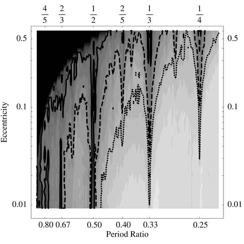
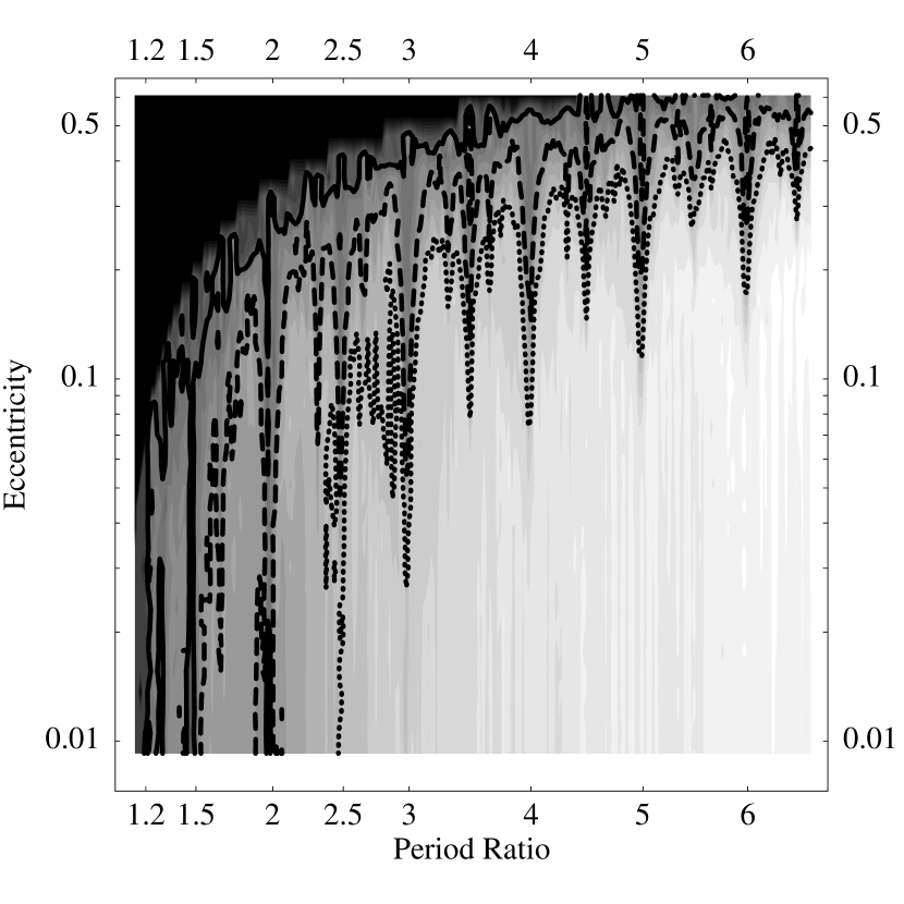
We see from these figures that near several mean-motion resonances, a secondary planet must be comparable to or less than the mass of the Earth for various values of the eccentricity. This is particularly manifest in the 2:1 and 3:2 mean motion resonances where this technique is most sensitive. Here, a secondary planet can be no larger than $5M_{\oplus}$ for an exterior perturber, $2M_{\oplus}$ for an interior perturber in the 3:2 resonance, and $<1M_{\oplus}$ for an interior perturber in the 2:1 resonance. These constraints are independent of the eccentricity of the perturber. For low initial eccentricity orbits ($e\sim 0.01$) the limits are as low as $0.2M_{\oplus}$, twice the mass of Mars.

We marginalized over eccentricity to compute limits on the presence of coplanar planetary companions in a 2:1 and 1:2 resonance with the transiting planet. Figure 7 shows the limits on planets within these resonances. Remarkably, the interior resonance can rule out at 3-$\sigma$ the presence of earth-mass bodies of any eccentricity within 0.5% of exact resonance (we have not included bodies with eccentricities large enough that their Hill spheres overlap with that of HD 209458b). The exterior resonance is slightly less sensitive, but can still rule out $\sim 2M_{\oplus}$ mass planets within 0.5% of resonance. We have checked for stability on timescales of several hundred orbits for resonant bodies, but have not carried out a longer timescale stability analysis.

Figure 7: Upper limit on the mass of any coplanar planetary companion present in the interior resonance (upper panel) or exterior (lower panel) 2:1 resonance with HD 209458b. The horizontal dashed line corresponds to an earth-mass plant.

4.1 Comparison with TrES-1 System

The first analysis of this sort was conducted for the TrES-1 planetary system (Steffen & Agol, 2005). That analysis used 11 transits observed with ground-based telescopes and was also able to probe for sub-earth mass planets. Those observations had an average timing uncertainty near 110 seconds–the most precise being 26 seconds. For this analysis of HD 209458b, being observed by HST, the average timing uncertainties are significantly smaller, with an average of 25 seconds (17 seconds for the STIS data).

The factor of four improvement in timing precision corresponds to a comparable improvement over the constraints on secondary planets in the HD209458 system. Figure 8 compares the limit on the mass of a companion planet for the TrES-1 system with that of the HD209458 system for perturbers with an eccentricity of 0.02. This figure shows that the constraint on the HD209458 system is similar in shape but markedly lower.

Figure 8: A comparison of the limits on a secondary planets obtained by TTV analysis for the TrES-1 system with 11 transits (upper curve) and the HD209458 system with 13 transits (lower curve). The primary distinction between the transit data for each system is that the ground-based TrES-1 observations have a timing uncertainty that is a factor of four, on average, larger than those of the HD209458 system, which were observed with HST.

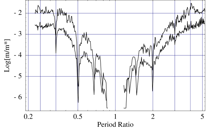
Though the space-based data can give tighter constraints for systems like TrES-1 and HD209458, figure 8 demonstrates the capacity that ground-based telescopes have to probe for secondary planets. The transit observations of the TrES-1 system were conducted on relatively modest telescopes (1m) and were not optimized for obtaining the time of transit. Even then, the best of the ground based observations (obtained using the 1.2m Fred Whipple telescope Charbonneau et al., 2005) have a timing precision that is essentially equal to the average uncertainty of the HST data. Thus, additional ground-based observations, with precision comparable to the best of those obtained for the TrES-1 system could readily probe for companions with masses less than that of the Earth that are trapped in low-order, mean-motion resonances.

4.2 Constraints Including Radial Velocity Measurements

Theoretical studies (Agol et al., 2005) indicate that high-precision radial velocity measurements should provide more stringent constraints than TTV for planets that are not in resonance. We therefore conducted a combined analysis that utilizes both the transit data and radial velocity data for this system. We used the radial velocity data that were published by Laughlin et al. (2005); discarding the data that they indicate were taken near transits.

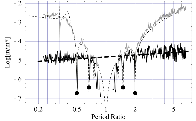
For this combined analysis we applied essentially the same algorithm that we used for the transit-only analysis and for the analysis of the TrES-1 system in Steffen & Agol (2005) with the difference that we compare the radial velocity data to a model with two Keplerian orbits with the parameters of the two planets. The change in the orbital elements of the planets due to non-resonant planet-planet interactions are small enough to not affect the radial velocities, justifying the use of Kepler’s equation. The results of our combined analysis are shown in Figure 9. We see from Figure 9 that our results are in good agreement with the theoretical predictions given in Agol et al. (2005) and Steffen & Agol (2005).

Figure 9: Limit on the mass of a low-eccentricity secondary planet in the HD209458 system. The solid, black curve is obtained from an analysis of transit times and radial velocity measurements simultaneously assuming that the orbits are initially circular. The gray curve is the result of an analysis of the transit times only, with the perturbing planet initially having an initial eccentricity of 0.02. The thin dashed curve is from a perturbation theory calculation and are given by equations (A7) and (A8) in Agol et al. (2005). The large dots are from equation (33) in Agol et al. (2005), although without the factor of 4.5 which is the difference between the peak TTV amplitude and the TTV amplitude for intitially exact $j$:$j+1$ resonance. The large, dashed line is from equation (2) in Steffen & Agol (2005) and is the expected limit from radial velocity measurements. The small, horizontal dashed line corresponds to the mass of the Earth.

5 Discussion

This investigation started as part of a larger quest for detecting terrestrial-mass planets orbiting main-sequence stars. Transits times are particularly sensitive to earth-mass planets in mean-motion resonance with the transiting planet. For the case of the HD 209458 system, we can rule out a wide range of terrestrial-mass planets based on the HST data analyzed and presented here. The paradigm of core accretion plus migration predicts that smaller planets ought to be trapped in resonance with larger, short-period planets (Zhou et al., 2005; Thommes, 2005). With the analysis of only two systems (HD 209458 and TrES-1), we cannot draw general conclusions, but in the next few years there will be likely be transit timing observations of all currently known transiting planets, so a significant constraint on the presence of resonant, earth-mass planets could be placed with this sample. In the process we have derived accurate parameters for the transiting planet which are broadly consistent with the analyses of other authors.

Despite its lofty position above the Earth’s atmosphere, it is apparent from these data that the Hubble Space Telescope is not ideally suited to timing transits. The main problem is its low-Earth orbit which causes occultation of the Sun leading to thermal variations within the orbit and causes occultation of the target star leading to gaps and re-pointing. The thermal variations cause sensitivity variations, while the gaps make a model for limb-darkening necessary to measure the transit times. If the data errors behaved according the Poisson statistics, the expected timing uncertainty for the STIS data would be of order 3-5 seconds, while the derived times are 4-5 times larger. The FGS data had a decreased sensitivity relative to the STIS data due to a lower count rate and the observation of each transit for only two or three orbits, an observing strategy which conserved Hubble time but was unsuited to the precise measurement of transit times. Future, precise measurements of transit times are possibly better carried out with satellites in Earth-trailing orbit, such as the Spitzer Space Telescope. Spitzer has the extra advantage that the infrared is less subject to limb-darkening; however, it would collect fewer photons as it has a smaller aperture and is observing past the peak of the photon count spectrum of G-type stars. In addition, ground-based observations with accurate relative photometry and coverage from observatories separated in longitude should make very accurate transit timing feasible from the ground. Finally, the Kepler satellite will discover a large number of transiting jupiters - the longer period planets will allow even more precise constraints on companions over a larger range of semi-major axis ratios (Holman & Murray, 2005). To contrain the presence of planets with mutual inclinations, more data points are required so that the model can accomodate more free parameters.

6 Acknowledgements

JHS acknowledges support from NASA Graduate Student Research Fellowship grant number NN605GO11H and from the Brinson Postdoctoral Fellowship. Support for this work was provided by NASA through grant number HST-AR-10637.01-A from the Space Telescope Science Institute which is operated by the Association of Universities for Research in Astronomy, Inc., under NASA contract NAS5-26555. We acknowledge Alfred Schultz and Wayne Kinzel for providing us with their preliminary reduction of the FGS data. We also thank Peter Hauschildt for making numerical limb-darkening models freely available. This paper has been assigned DOE preprint number FERMILAB-PUB-06-279-A-CD.

References

- Agol et al. (2005) Agol E., Steffen J., Sari R., Clarkson W., 2005, MNRAS, 359, 567
- Brown et al. (2001) Brown T. M., Charbonneau D., Gilliland R. L., Noyes R. W., Burrows A., 2001, ApJ, 552, 699
- Charbonneau et al. (2005) Charbonneau D., Allen L. E., Megeath S. T., Torres G., Alonso R., Brown T. M., Gilliland R. L., Latham D. W., Mandushev G., O’Donovan F. T., Sozzetti A., 2005, ApJ, 626, 523
- Charbonneau et al. (2006) Charbonneau D., Brown T. M., Burrows A., Laughlin G., 2006, ArXiv Astrophysics e-prints: astro-ph/0603376
- Charbonneau et al. (2000) Charbonneau D., Brown T. M., Latham D. W., Mayor M., 2000, ApJL, 529, L45
- Charbonneau et al. (2002) Charbonneau D., Brown T. M., Noyes R. W., Gilliland R. L., 2002, ApJ, 568, 377
- Claret & Hauschildt (2003) Claret A., Hauschildt P. H., 2003, A & A, 412, 241
- Cody & Sasselov (2002) Cody A. M., Sasselov D. D., 2002, ApJ, 569, 451
- Cowell (1984) Cowell W. R., ed. 1984, Sources and Development of Mathematical Software. Prentice-Hall, Upper Saddle River, NJ 07458, USA
- Deming et al. (2005) Deming D., Seager S., Richardson L. J., Harrington J., 2005, Nature, 434, 740
- Guillot et al. (2006) Guillot T., Santos N. C., Pont F., Iro N., Melo C., Ribas I., 2006, A&A, 453, L21
- Henry et al. (2000) Henry G. W., Marcy G. W., Butler R. P., Vogt S. S., 2000, ApJL, 529, L41
- Holman & Murray (2005) Holman M. J., Murray N. W., 2005, Science, 307, 1288
- Knutson et al. (2006) Knutson H., Charbonneau D., Noyes R. W., Brown T. M., Gilliland R. L., 2006, ArXiv Astrophysics e-prints: astro-ph/0603542
- Laughlin et al. (2005) Laughlin G., Marcy G. W., Vogt S. S., Fischer D. A., Butler R. P., 2005, ApJL, 629, L121
- Mandel & Agol (2002) Mandel K., Agol E., 2002, ApJL, 580, L171
- Mayor & Queloz (1995) Mayor M., Queloz D., 1995, Nature, 378, 355
- Schultz et al. (2004) Schultz A. B., Kinzel W., Kochte M., Jordan I. J. E., Hamilton F., Henry G., Vogt S., Bruhweiler F., Storrs A., Hart H. M., Bennum D., Rassuchine J., Rodrigue M., Hamilton D. P., Welsh W. F., Taylor D. C., 2004, in Holt S. S., Deming D., eds, AIP Conf. Proc. 713: The Search for Other Worlds HST/FGS Photometry of Planetary Transits of HD 209458. pp 161–164
- Steffen & Agol (2005) Steffen J. H., Agol E., 2005, MNRAS, 364, L96
- Thommes (2005) Thommes E. W., 2005, ApJ, 626, 1033
- Valenti & Fischer (2005) Valenti J. A., Fischer D. A., 2005, ApJS, 159, 141
- Wittenmyer et al. (2005) Wittenmyer R. A., Welsh W. F., Orosz J. A., Schultz A. B., Kinzel W., Kochte M., Bruhweiler F., Bennum D., Henry G. W., Marcy G. W., Fischer D. A., Butler R. P., Vogt S. S., 2005, ApJ, 632, 1157
- Zhou et al. (2005) Zhou J.-L., Aarseth S. J., Lin D. N. C., Nagasawa M., 2005, ApJL, 631, L85