Two strong-lensing clusters
confront universal dark-matter profiles

Abstract

In the galaxy clusters SSDS J1004+411 and ACO 1689, a large number of multiply-imaged background objects have recently been observed. We use these data to map the projected mass distribution in the inner regions of these clusters. The source redshifts in these clusters span a large range, which eliminates the degeneracies that plague nearly all lensing work. As a result the mass maps are very well-constrained, despite very weak prior assumptions. ACO 1689 lenses so many objects that we can afford to map it twice using disjoint sets of images, thus verifying our internal error estimates. We then deproject the mass maps (pretending for this purpose that they are spherical) and obtain inner profiles consistent with $\rho\propto r^{-1}$ and indistinguishable from recent cold dark matter simulations. Assuming that baryons make only a small difference to the profile outside $\sim 10{\rm\;kpc}$, these results support the prediction of a universal inner profile for dark matter structures, independent of any parametrization of that profile.

1 Why inner profiles of clusters?

A key prediction of heirarchical clustering dominated by cold dark matter is that virialized structures have a universal density profile. Although there is still no first-principles derivation of a universal profile, $N$-body simulations and phenomenological models both consistently indicate that such a profile exists.

The best-known candidate for a universal profile remains the original proposal

$$\rho\propto(r/r_{\hbox{\tiny{s}}})^{-1}(1+r/r_{\hbox{\tiny{s}}})^{-2}$$ (1)

from Navarro et al. (1997), but it is gradually being superseded. In recent simulations —see for example, Fig. 3 of Navarro et al. (2004)— NFW remains a reasonable fit to individual simulated halos, but an ensemble of halos shows the steepness changing gradually with no distinct $r_{\hbox{\tiny{s}}}$. Graham et al. (2005) discuss alternative parametrizations. The smallest resolved scales in current dark-matter simulations have $\rho\sim r^{-1.2\pm 0.2}$ (Diemand et al., 2004). The total mass profile would be somewhat steeper at the smallest radii, because of the infall of baryons and the response of the dark-matter to the baryons. The latter effect is generally modelled as adiabatic contraction (Blumenthal et al., 1986; Gnedin et al., 2004).

These results motivate research on the inner profiles of real clusters.

2 Why J1004+411 and ACO 1689?

Testing predicted universal profiles against observations seems straightforward at first. Well-known strategies are to

1. put observed velocity dispersions through the Jeans equation to infer a density profile, or

2. fit a mass model to lensing data, or

3. invert an observed x-ray profile through the hydrostatic equilibrium equation.

The first two approaches, and to a lesser extent the third, have all been followed in the literature, but the conclusions remain unclear. For example: Łokas et al. (2006) using method (1) find NFW profiles satisfactory, whereas Sand et al. (2004) using a combination of (1) and (2) find inner profiles significantly shallower than NFW.

Evidently there are major uncertainties involved in extracting a mass profile. It is useful to get some insight into what the uncertainties are, and hence how robust different methods are likely to be. By considering the basic equations involved, we can identify problematic operations that either amplify noise or introduce systematic errors. Let us call them gremlins.

The first gremlin appears in deprojecting an observed quantity, via the well-known Abel integral

$$\rho(r)=-\frac{1}{\pi}\int_{r}^{\infty}\frac{d\Sigma(R)}{dR}\frac{dR}{\sqrt{R^{2}-r^{2}}}.$$ (2)

In this case, differentiating an observed $\Sigma(R)$ amplifies the noise. Smoothing $\Sigma(R)$ will suppress the noise of course, but will replace it with a systematic error. However, the integral tends to suppress the noise somewhat, so this gremlin is comparatively benign.

Next, consider Jeans equation for spherical systems

$$GM(r)=\frac{r^{2}}{\rho_{\hbox{\tiny{l}}}}\frac{d}{dr}(\rho_{\hbox{\tiny{l}}}\sigma_{r}^{2})-2r(\sigma_{r}^{2}-\sigma_{t}^{2})$$ (3)

relating the luminous density $\rho_{\hbox{\tiny{l}}}$ and velocity dispersions to the mass profile. Since $\sigma_{r}$ and $\sigma_{t}$ cannot be directly observed, they need to be related to the projected dispersion somehow. This introduces a second gremlin: assumptions about anisotropy produce a systematic error; deriving the anisotropy from higher velocity moments (Łokas et al., 2006) introduces noise. The derivative in Eq. (3) is a third gremlin.

For x-ray emitting gas in hydrostatic equilibrium, the temperature profile $T(r)$ and gas density profile $\rho_{\hbox{\tiny{g}}}(r)$ are related to the total mass profile by

$$GM(r)=\frac{kT}{\mu m_{p}}r^{2}\left(\frac{1}{T}\frac{dT}{dr}+\frac{1}{\rho_{\hbox{\tiny{g}}}}\frac{d\rho_{\hbox{\tiny{g}}}}{dr}\right)$$ (4)

where $\mu_{p}$ is the proton mass and $\mu$ the particle weight. Here the first gremlin appears in deprojecting for $T(r)$ and $\rho_{\hbox{\tiny{g}}}(r)$, while the third gremlin appears in another guise in the derivatives of $T$ and $\rho_{\hbox{\tiny{g}}}$.

Lensing is free of the second and third gremlins. Moreover it provides one simple and robust constraint on mass profiles. Central images are extinguished by an isothermal or steeper cusp (Evans & Wilkinson, 1998), and the fact that clusters commonly host central images implies that clusters are shallower than isothermal (Subramanian et al., 2000).

Lensing, however, introduces a new gremlin, namely lensing degeneracies. Consider the equation for the arrival time

$$\tau(\hbox{\boldmath{$\theta$}}_{\hbox{\tiny{I}}};\hbox{\boldmath{$\theta$}}_{\hbox{\tiny{S}}})={\textstyle\frac{1}{2}}(\hbox{\boldmath{$\theta$}}_{\hbox{\tiny{I}}}-\hbox{\boldmath{$\theta$}}_{\hbox{\tiny{S}}})^{2}-2c_{\hbox{\tiny{LS}}}\nabla^{-2}\kappa(\hbox{\boldmath{$\theta$}}_{\hbox{\tiny{I}}})$$ (5)

which represents the time delay for a virtual photon originating from a source at sky position $\hbox{\boldmath{$\theta$}}_{\hbox{\tiny{S}}}$ and getting deflected at the lens so that the observer sees it coming from sky-position $\hbox{\boldmath{$\theta$}}_{\hbox{\tiny{I}}}$. The first term on the right of Eq. (5) is the geometrical path difference between a deflected and undeflected photon trajectory, and the last term is the Shapiro time delay. The whole equation is dimensionless: $\tau$ is a scaled time delay and $\kappa$ is a scaled surface density, the coordinates are in radians, while $c_{\hbox{\tiny{LS}}}\sim 1$ is a ratio of distances depending on lens and source redshifts. The gradient of $\tau$ with respect to $\hbox{\boldmath{$\theta$}}_{\hbox{\tiny{I}}}$ gives the lens equation, and the matrix of second derivatives is the inverse magnification. Thus, image positions in strong lensing constrain the first derivative of $\tau$ while shear or magnification in weak or strong lensing constrain the second derivative. These derivatives are not gremlins, because no differentiation of data is involved. But let us rewrite the equation as

$$\tau=2\,\nabla^{-2}(1-c_{\hbox{\tiny{LS}}}\kappa)-\hbox{\boldmath{$\theta$}}_{\hbox{\tiny{I}}}\cdot\hbox{\boldmath{$\theta$}}_{\hbox{\tiny{S}}}$$ (6)

where we have expanded the geometrical part and then discarded a $\hbox{\boldmath{$\theta$}}_{\hbox{\tiny{S}}}^{2}$ term since it has no optical effect. If $c_{\hbox{\tiny{LS}}}$ is a constant (that is, there is only one source redshift) then we may rescale Eq. (6) by some positive factor $\lambda$:

$$\tau\leftarrow\lambda\tau,\quad\hbox{\boldmath{$\theta$}}_{\hbox{\tiny{S}}}\leftarrow\lambda\hbox{\boldmath{$\theta$}}_{\hbox{\tiny{S}}},\quad(1-c_{\hbox{\tiny{LS}}}\kappa)\leftarrow\lambda(1-c_{\hbox{\tiny{LS}}}\kappa).$$ (7)

Eq. (7) amounts to redefining the contour spacing in Blandford & Narayan’s Fig. 2, without changing the figure — the observables don’t change, but the $\kappa$ profile becomes steeper (if $\lambda>1$ or shallower (if $\lambda<1$). This is our fourth, and perhaps most vicious, gremlin. The case where $\lambda$ is constant is well known as a steepness degeneracy (Falco et al., 1985), but in fact $\lambda$ need not even be constant (Saha, 2000; Zhao & Qin, 2003; Saha & Williams, 2006). Having a range of source redshifts breaks the degeneracies (Abdelsalam et al., 1998b); having number counts of weakly lensed objects breaks the main steepness degeneracy (Dye et al., 2002).

The above arguments indicate that lens reconstructions with special attention to breaking lensing degeneracies are likely to provide the most robust mass profiles. The clusters which have been so analyzed are ACO 2218 (Kneib et al., 1996; Abdelsalam et al., 1998b) ACO 370 (Abdelsalam et al., 1998a), ACO 1689 (Dye et al., 2002; Broadhurst et al., 2005; Diego et al., 2005; Zekser et al., 2006; Halkola et al., 2006), and J1004+411 (Sharon et al., 2005). The first two have double-peaked mass distributions, evidently from ongoing mergers. That leaves the last two lensing clusters as worthy of special attention.

3 Mass profiles

We will now use the excellent recent strong-lensing observations by Sharon et al. (2005) on J1004+411 and by Broadhurst et al. (2005) on ACO 1689 to map the mass distribution in the inner regions of these clusters. As we noted above, these data have already made into models by the observing authors and others. Our work, however, goes further than previous models because (i) rather than fitting one or a few models to the data, we generate large ensembles of models exploring the possible mass distributions that can reproduce the data; (ii) we compare results from independent data sets to test for consistency; and (iii) we deproject the surface density profiles non-parametrically for a better comparison with simulations.

Our technique is implemented in the PixeLens code, originally developed for galaxy lenses (Saha & Williams, 2004), but now enhanced to use multiple source-redshifts. Given the multiple-image data, the program generates an ensemble of 400 models that each (a) reproduce the lensing data exactly, and (b) are consistent with a given prior on the mass map. The model ensemble automatically provides Bayesian uncertainties on the mass map or any derived quantity. We assume a concordance cosmology ($K=0,\Omega_{\hbox{\tiny{m}}}=0.3,w=-1$) with $H_{0}^{-1}=14\rm\,Gyr$. Cosmological parameters enter into the the mass and distance scales, but not the profiles themselves.

The prior we assume is the same as in Saha & Williams (2004) —basically it requires that that the surface density be non-negative and centrally concentrated, with substructure allowed— but with one difference: we remove the requirement that $\Sigma$ be steeper than $R^{-0.5}$ (which was motivated by galaxy dynamics) and require only that the cylindrically-averaged $\Sigma$ decrease with $R$. We measure $R$ from the center of the brightest cluster galaxy, so the mass peak is modeled to coincide with the light peak. In some lensing clusters mass and light peaks have been inferred to be offset tens of kpc (Abdelsalam et al., 1998a, b), but in J1004+411 and ACO 1689 the central lensed images indicate that any such offset is small.

The requirement of exact fits to the image data leaves PixeLens currently unable to handle all the multiple-image data on ACO 1689. (The problem is accumulation of roundoff error.) Nevertheless, we can make a virtue of this by splitting the data into two independent sets. Accordingly, we present three mass reconstructions:

1. J1004+411 ($z_{\hbox{\tiny{L}}}=0.68$) reconstructed using 13 images coming from 4 sources ($z_{\hbox{\tiny{S}}}=1.73$ to 3.33),

2. ACO 1689 ($z_{\hbox{\tiny{L}}}=.18$) reconstructed using 30 images of 9 sources ($z_{\hbox{\tiny{S}}}=1.74$ to 4.52), and

3. ACO 1689 again, reconstructed using 28 images of 7 other sources ($z_{\hbox{\tiny{S}}}=1.57$ to 5.16).

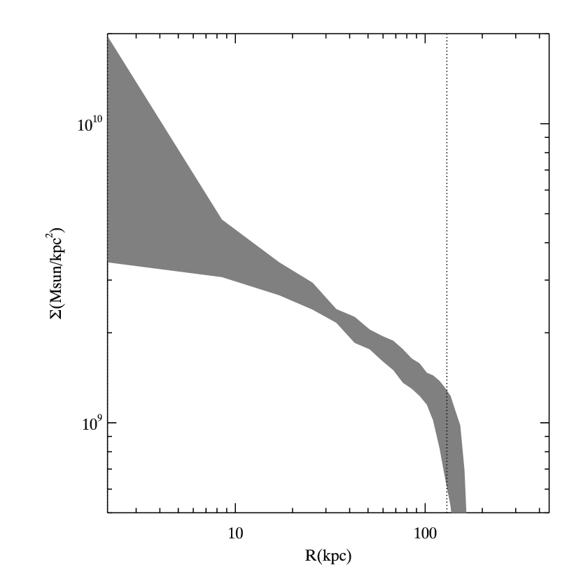
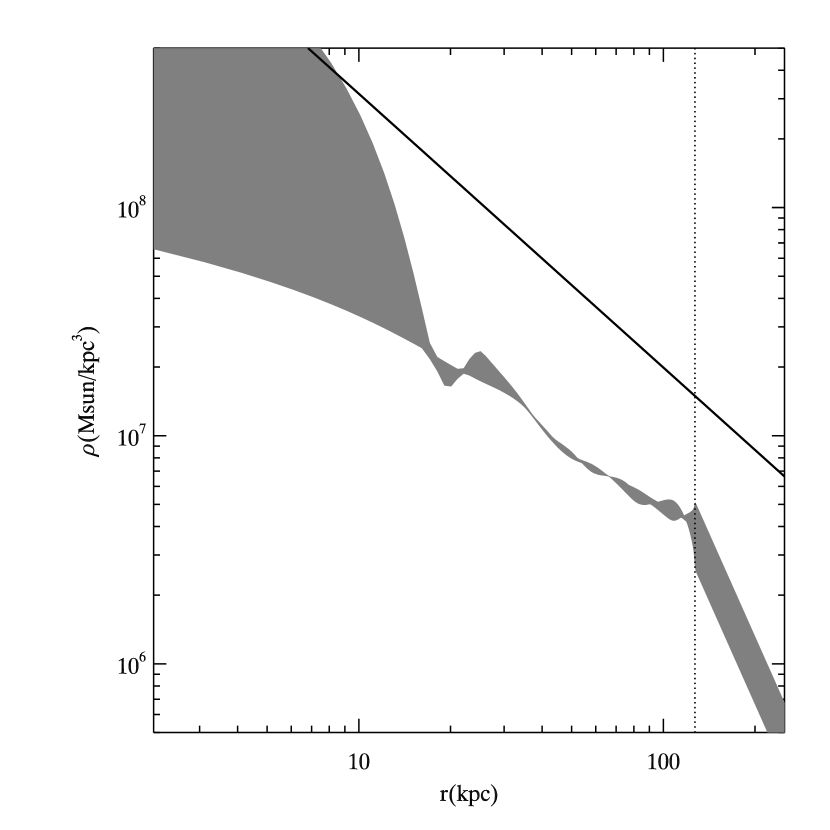
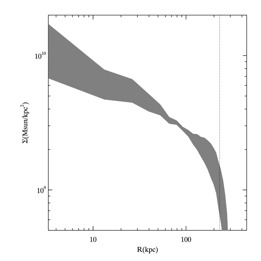
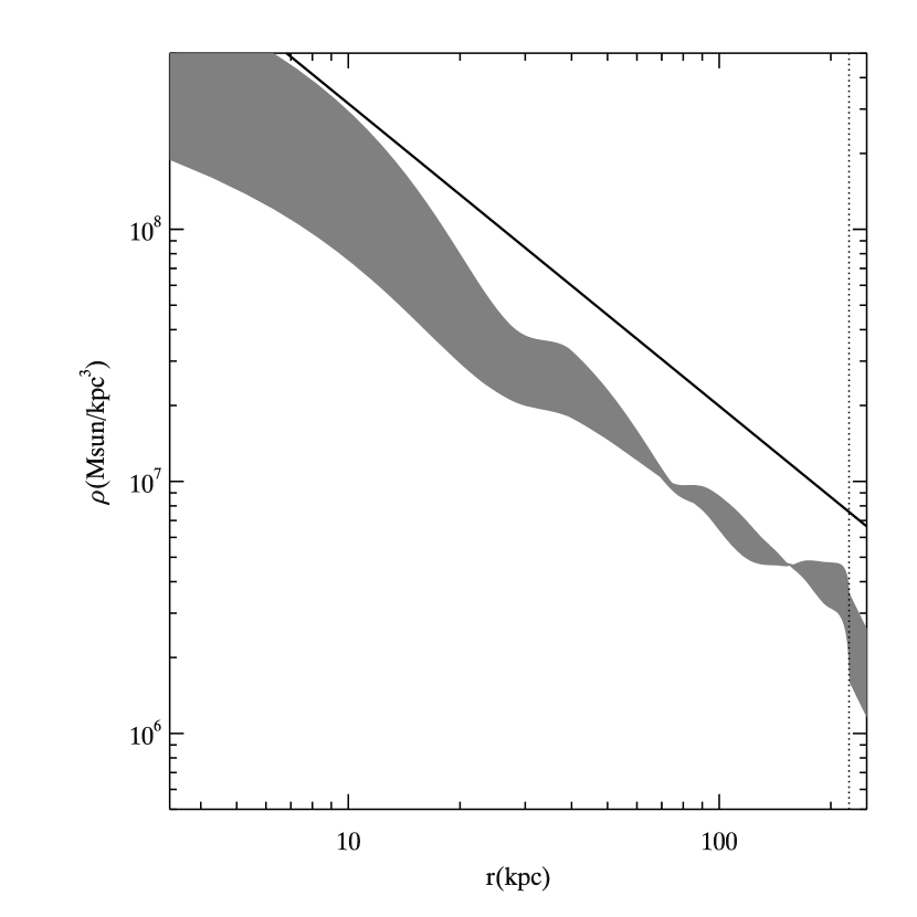
Figure 1 packs all the results of this paper. To the left we show three ensemble-average mass maps. Both clusters appear fairly round, but have some substructure, such as a feature to the NE in ACO 1689. In this paper we concentrate on radial dependence, leaving substructure for later work.

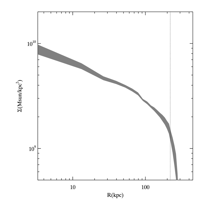
The middle column of the figure shows the cylindrically-averaged surface density $\Sigma(R)$, with 90%-confidence uncertainties derived from the model-ensemble. In each case we see a shallow and tightly constrained profile in the inner region, and moreover the two profiles for ACO 1689 from independent image-sets agree. (The profile beyond the outermost image is to be disregarded; there PixeLens has no data to work with and simply makes the profile fall smoothly to zero at the edge of the map.) The enclosed mass agrees with previous strong-lensing estimates but is about a factor of two higher than current models for the x-ray gas give (Andersson & Madejski, 2004). The improvement upon our earlier reconstructions of J1004+411 Williams & Saha (2004) using a single 4-image background object is remarkable: then we concluded that the lens was consistent with NFW, but even a profile as steep as $R^{-1.3}$ was not excluded; now simply inspecting the upper middle panel of Fig. 1 shows that this cluster is shallower than $1/R$.

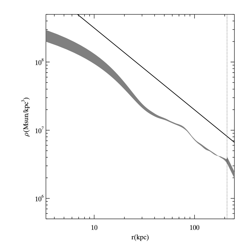
To the right of the figure we show $\rho(r)$, derived from $\Sigma(R)$ using Eq. (2). To evaluate the numerical derivative and then the integral, we fit a spline to $\Sigma$ up to the $R$ of the outermost image and assumed $\Sigma\propto R^{-2}$ outside. (The result is not sensitive to the assumed outside slope, or to the boundary between spline and $R^{-2}$, provided the latter is not beyond the image region.) Here again we show ensemble-derived uncertainties, which in this case are probably too small, because substructure will introduce systematic errors through the derivative in Eq. (2). With this caveat, our constraints on the steepness between 10 kpc and the outermost image are as follows: J1004+411 is best fit by $\rho\propto r^{-0.9}$ but the uncertainty bands shown allow $r^{-0.8}$ to $r^{-1.2}$, while ACO 1689 is best fit by $\rho\propto r^{-1.15}$ but the uncertainty bands allow $r^{-1.0}$ to $r^{-1.25}$. These values are typical of the inner slopes in Table 3 of Diemand et al. (2004). The right column of Fig. 1 is also comparable to their Fig. 4. For ACO 1689 we have also attempted to model the change in the profile due to adiabatic contraction, using estimated gas density from Fig. 9 of Andersson & Madejski (2004), but the difference is smaller than our estimated uncertainties. It appears that baryons make a difference of at most 10%, which is of the same order as the substructure. We conclude that, within current uncertainties, the inner slopes in these lensing clusters and in simulations are indistinguishable.

4 Discussion

In this paper we have used recent strong lensing observations having multiple source-redshifts (Sharon et al., 2005; Broadhurst et al., 2005) to reconstruct the inner density profiles of two clusters in a non-parametric way. These inner density profiles show remarkable agreement with simulations of CDM halos. Although we have disregarded the secondary questions of baryons (not included in simulations at this scale) and substructure (present in both the real Universe and simulated ones), our results arguably confirm an important prediction of heirarchical structure formation.

But why are the profiles the way they are? There is still nothing approaching a first-principles derivation of a universal profile, though there are several interesting ideas. The only exactly solved case is self-similar spherical collapse, but that implies $\rho\propto r^{-2.25}$ (Fillmore & Goldreich, 1984; Bertschinger, 1985) which is too steep. Subramanian et al. (2000) propose a cunning variant involving merging self-similar proto-halos into a Matreshka-like heirarchy, resulting in a composite halo with a shallow inner slope; but their mechanism relies on undigested merging. Several other scenarios involving spherical collapse have also been studied, and recently Lu et al. (2006) proposed a phenomenological 1D model that produces an $r^{-1}$ inner slope and an $r^{-3}$ outer slope. Finally, one numerical result is especially intriguing: in CDM collapse simulations the surrogate phase-space density $\rho/\sigma^{3}\propto r^{-\alpha}$ (Taylor & Navarro, 2001; Barnes et al., 2005). Combining this relation with the Jeans equation gives $\rho\propto r^{-0.8}$ asymptotically for small $r$ (Austin et al., 2005; Hansen et al., 2006; Dehnen & McLaughlin, 2005). The total mass profile at very small $r$ would be steeper than this because of the baryons, and anyway our results do not have the resolution to test for this yet. But it remains an interesting prediction.

Figure 1: Mass maps and profiles for J1004+411 and for ACO 1689. Left column: Ensemble-average mass maps together with the lensed image positions. Panels are oriented as North-up/East-left. Ticks correspond to $20{\rm\;kpc}$ for J1004+411 and $100{\rm\;kpc}$ for ACO 1689. Contour steps are $0.5\times 10^{9}M_{\odot}\;\rm kpc^{-2}$ for J1004+411 and $10^{9}M_{\odot}\;\rm kpc^{-2}$ for ACO 1689. Middle column: $\Sigma(R)$ for the mass maps in in the left column, together with 90% uncertainties. The vertical lines to the right show $R$ for the outermost image. Right column: Density profiles, derived by deprojecting the profiles from the middle column. The sloped line shows $\rho\propto r^{-1.2}$.

References

- Abdelsalam et al. (1998a) Abdelsalam, H. M., Saha, P., & Williams, L. L. R. 1998a, MNRAS, 294, 734
- Abdelsalam et al. (1998b) —. 1998b, AJ, 116, 1541
- Andersson & Madejski (2004) Andersson, K. E. & Madejski, G. M. 2004, ApJ, 607, 190
- Austin et al. (2005) Austin, C. G., Williams, L. L. R., Barnes, E. I., Babul, A., & Dalcanton, J. J. 2005, ApJ, 634, 756
- Barnes et al. (2005) Barnes, E. I., Williams, L. L. R., Babul, A., & Dalcanton, J. J. 2005, ApJ, 634, 775
- Bertschinger (1985) Bertschinger, E. 1985, ApJS, 58, 39
- Blandford & Narayan (1986) Blandford, R. & Narayan, R. 1986, ApJ, 310, 568
- Blumenthal et al. (1986) Blumenthal, G. R., Faber, S. M., Flores, R., & Primack, J. R. 1986, ApJ, 301, 27
- Broadhurst et al. (2005) Broadhurst, T., Benítez, N., Coe, D., Sharon, K., Zekser, K., White, R., Ford, H., Bouwens, R., Blakeslee, J., Clampin, M., Cross, N., Franx, M., Frye, B., Hartig, G., Illingworth, G., Infante, L., Menanteau, F., Meurer, G., Postman, M., Ardila, D. R., Bartko, F., Brown, R. A., Burrows, C. J., Cheng, E. S., Feldman, P. D., Golimowski, D. A., Goto, T., Gronwall, C., Herranz, D., Holden, B., Homeier, N., Krist, J. E., Lesser, M. P., Martel, A. R., Miley, G. K., Rosati, P., Sirianni, M., Sparks, W. B., Steindling, S., Tran, H. D., Tsvetanov, Z. I., & Zheng, W. 2005, ApJ, 621, 53
- Dehnen & McLaughlin (2005) Dehnen, W. & McLaughlin, D. E. 2005, MNRAS, 363, 1057
- Diego et al. (2005) Diego, J. M., Sandvik, H. B., Protopapas, P., Tegmark, M., Benítez, N., & Broadhurst, T. 2005, MNRAS, 362, 1247
- Diemand et al. (2004) Diemand, J., Moore, B., & Stadel, J. 2004, MNRAS, 353, 624
- Dye et al. (2002) Dye, S., Taylor, A. N., Greve, T. R., Rögnvaldsson, Ö. E., van Kampen, E., Jakobsson, P., Sigmundsson, V. S., Gudmundsson, E. H., & Hjorth, J. 2002, A&A, 386, 12
- Evans & Wilkinson (1998) Evans, N. W. & Wilkinson, M. I. 1998, MNRAS, 296, 800
- Falco et al. (1985) Falco, E. E., Gorenstein, M. V., & Shapiro, I. I. 1985, ApJ, 289, L1
- Fillmore & Goldreich (1984) Fillmore, J. A. & Goldreich, P. 1984, ApJ, 281, 1
- Gnedin et al. (2004) Gnedin, O. Y., Kravtsov, A. V., Klypin, A. A., & Nagai, D. 2004, ApJ, 616, 16
- Graham et al. (2005) Graham, A. W., Merritt, D., Moore, B., Diemand, J., & Terzic, B. 2005, astro-ph/0509417
- Halkola et al. (2006) Halkola, A., Seitz, S., & Panella, M. 2006, astro-ph/0605470
- Hansen et al. (2006) Hansen, S. H., Moore, B., & Stadel, J. 2006, in EAS Publications Series, 33–36
- Kneib et al. (1996) Kneib, J.-P., Ellis, R. S., Smail, I., Couch, W. J., & Sharples, R. M. 1996, ApJ, 471, 643
- Łokas et al. (2006) Łokas, E. L., Wojtak, R., Gottlöber, S., Mamon, G. A., & Prada, F. 2006, MNRAS, 367, 1463
- Lu et al. (2006) Lu, Y., Mo, H. J., Katz, N., & Weinberg, M. D. 2006, MNRAS, 368, 1931
- Navarro et al. (1997) Navarro, J. F., Frenk, C. S., & White, S. D. M. 1997, ApJ, 490, 493
- Navarro et al. (2004) Navarro, J. F., Hayashi, E., Power, C., Jenkins, A. R., Frenk, C. S., White, S. D. M., Springel, V., Stadel, J., & Quinn, T. R. 2004, MNRAS, 349, 1039
- Saha (2000) Saha, P. 2000, AJ, 120, 1654
- Saha & Williams (2004) Saha, P. & Williams, L. L. R. 2004, AJ, 127, 2604
- Saha & Williams (2006) —. 2006, ApJ in press and astro-ph/0608496
- Sand et al. (2004) Sand, D. J., Treu, T., Smith, G. P., & Ellis, R. S. 2004, ApJ, 604, 88
- Sharon et al. (2005) Sharon, K., Ofek, E. O., Smith, G. P., Broadhurst, T., Maoz, D., Kochanek, C. S., Oguri, M., Suto, Y., Inada, N., & Falco, E. E. 2005, ApJ, 629, L73
- Subramanian et al. (2000) Subramanian, K., Cen, R., & Ostriker, J. P. 2000, ApJ, 538, 528
- Taylor & Navarro (2001) Taylor, J. E. & Navarro, J. F. 2001, ApJ, 563, 483
- Williams & Saha (2004) Williams, L. L. R. & Saha, P. 2004, AJ, 128, 2631
- Zekser et al. (2006) Zekser, K. C., White, R. L., Broadhurst, T. J., Benítez, N., Ford, H. C., Illingworth, G. D., Blakeslee, J. P., Postman, M., Jee, M. J., & Coe, D. A. 2006, ApJ, 640, 639
- Zhao & Qin (2003) Zhao, H. & Qin, B. 2003, ApJ, 582, 2