Color Tomography

Abstract

Lensing tomography with multi-color imaging surveys can probe dark energy and the cosmological power spectrum. However accurate photometric redshifts for tomography out to high redshift require imaging in five or more bands, which is expensive to carry out over thousands of square degrees. Since lensing makes coarse, statistical use of redshift information, we explore the prospects for tomography using limited color information from two or three band imaging. With an appropriate calibration sample, we find that it is feasible to create up to four redshift bins using imaging data in just the $g$, $r$ and $i$ bands. We construct such redshift sub-samples from mock catalogs by clustering galaxies in color space and discarding regions with poorly-defined redshift distributions. The loss of galaxy number density decreases the accuracy of lensing measurements, but even losing half or more of the galaxies is not a severe loss for large area surveys. We estimate the errors on lensing power spectra and dark energy parameters with color tomography and discuss trade-offs in survey area and filter choice. We discuss the systematic errors that may change our conclusions, especially the information needed to tackle intrinsic alignments.

1 Introduction

Over the last decade a concordance model has emerged in cosmology in which about two-thirds of the energy density of the universe today may be in the form of “dark energy”. This explains the observation that we reside in an accelerating universe (Riess et al., 1998; Perlmutter et al., 1999). Despite its importance to the formation and evolution of the universe there are no compelling theories that explain the energy density nor the properties of the dark energy.

To address questions about the nature of dark energy a number of ambitious wide-field optical and infrared imaging surveys have been proposed. These range from space-based missions in the optical and infrared, such as the Supernova Acceleration Probe (SNAP, proposed as the space-based Joint Dark Energy Mission (JDEM)), to ground-based surveys such as the Panoramic Survey Telescope & Rapid Response System (Pan-STARRS), the Dark Energy Survey (DES), the Large Synoptic Sky Survey (LSST) and others. Each of these missions approaches the study of dark energy using multiple, complementary observational probes: gravitational weak lensing (WL) to study the growth of structure and geometry, baryon oscillations to measure the angular diameter distance vs. redshift relation and Type Ia supernovae to measure the luminosity distance vs. redshift relation.

In this paper we focus on one of these probes, weak lensing, and how the design of a survey might impact its scientific value for constraining dark energy. Observations to date have succeeded in measuring the amplitude $\sigma_{8}$ of the $z\approx 0$ dark matter power spectrum to $\approx 10\%$ accuracy (cf. Jarvis et al. (2005); Hoekstra et al. (2005) and references therein) by surveying $\simeq 100$ deg² of sky. To constrain the equation of state of dark energy requires that we improve the accuracy of these measures by close to an order of magnitude. To achieve this deep imaging surveys have been proposed that cover surveys of 1,000-20,000 square degrees in 5-6 filters. There is, however, a natural trade off in the design of these surveys; depth vs number of filters vs area surveyed. To date the appropriate weighting of these components is not fully understood. For example, given the time and cost of a survey, does a large area, shallow survey in a small number of filters provide more scientific return than a deep survey in a large number of filters but sampling only a few hundred square degrees?

One of the primary requirements for any lensing application is the need for redshift information on the source galaxies. In the first studies of lensing only the statistical redshift distribution was available, but now surveys aim to get photometric redshifts (Connolly et al. 1995; hereafter photo-z’s) for individual galaxies. Accurate photo-z information enables new qualitative and quantitative advances in lensing. Conversely photo-z errors can be a limiting systematic in the use of lensing for precision cosmology.

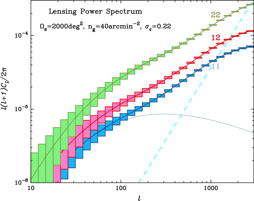
Lensing tomography refers to the use of depth information in the source galaxies to get three-dimensional information on the lensing mass (Hu, 1999). By binning source galaxies in photo-z bins, the evolution of the lensing power spectrum can be measured. This greatly improves the sensitivity of lensing to dark energy in cosmological applications. The lensing power spectra measured from two redshift bins is shown in Figure 1. The two auto-spectra and the cross-spectrum, along with expected statistical errors, are shown. The relative shift in the amplitudes of the lensing spectra is sensitive to the properties of dark energy. It depends on both distances and the growth of structure, thus enabling tests of dark energy or modified gravity explanations for the cosmic acceleration. In Figure 1, the amplitude shifts of the three spectra (for a given cosmological model) depend on the mean redshifts and widths of the two photo-z bins; clearly any errors in the bin redshifts will degrade the ability to discriminate cosmological models.

Thus the use of broadband multicolor photometry to estimate the distances of galaxies (i.e. photometric redshifts; henceforth abbreviated as photo-z’s) is critical to the use of lensing for dark energy studies. The capability of these surveys to meet their scientific goals will depend on our ability to characterize the uncertainties present within photometric redshift estimates, i.e. the scatter, bias and fraction of outliers. Photometric redshifts must be calibrated with an appropriate sample of spectroscopic redshifts (Huterer et al. 2005; Ma et al. 2005). This may be done more cheaply by using auto- and cross-correlations of photometric and spectroscopic redshifts samples (Newman, 2006; Schneider et al., 2006), which can also be used to estimate the redshift distribution for a galaxy sample where the calibration data is incomplete (see also Zhan & Knox 2006).

In this paper we study the possibility of doing lensing tomography from limited color information. Imaging in five or more bands is needed for well-characterized photo-z’s of galaxies extending beyond $z\sim 1$. We consider here whether lensing tomography can be carried out from a wide-area imaging survey in just two or three filters, along with a relatively small calibration sample that provides the statistical redshift distributions in all parts of the color space. These can be used to create a few sub-samples of the full galaxy sample that occupy distinct redshift bins, while discarding galaxies with colors that lead to badly defined redshift distributions. Since lensing does not require redshift bins much narrower than $0.2$-$0.4$ in redshift, and does not need a full or fair sample of the galaxy population, there is reason to expect that limited color information may be sufficient for tomography. We use a mock catalog of galaxies with known redshifts to see how well one can make cosmological measurements with this approach, taking into account statistical errors in lensing measurements. In a future paper we will expand upon this analysis to include various sources of systematic errors in colors/photo-z’s and in the lensing measurements.

In Section 2 we describe the formalism for computing lensing power spectra given the redshift distribution of a galaxy sample. In Section 3 the mock catalog used for our study is described. Section 4 contains the results on how well one can do with color cuts in making well separated redshift distributions for galaxy sub-samples. The errors on the power spectra and dark energy parameters are compared with the forecasts for idealized photo-z’s. In Section 5 we discuss the prospects for tomography with color cuts from imaging in a limited number of filters – which we call color tomography.

2 Lensing Formalism

We will use the shear power spectrum as the lensing statistic for dark energy constraints. Similar results can be obtained using two-point correlations and the mass aperture statistic. The key element in constraining dark energy is to use source galaxies in different redshift bins to probe the evolution of mass fluctuations and the geometric factors involved in lensing.

2.1 Preliminaries: cosmology and weak lensing

We work in the context of spatially flat cold dark matter models for structure formation. The expansion history of the universe is given by the scale factor $a(t)$ in a homogeneous and isotropic universe. The expansion rate, the Hubble parameter, is given in terms of the matter density $\Omega_{\rm m}$ (the cold dark matter plus the baryons) and dark energy density $\Omega_{\rm de}$ at present (in units of the critical density $3H_{0}^{2}/(8\pi G)$, where $H_{0}=100~{}h~{}{\rm km}~{}{\rm s}^{-1}~{}{\rm Mpc}^{-1}$ is the Hubble parameter at present) by

$$H^{2}(a)=H_{0}^{2}\left[\Omega_{\rm m}a^{-3}+\Omega_{\rm de}e^{-3\int^{a}_{1}da^{\prime}(1+w(a^{\prime}))/a^{\prime}},\right]$$ (1)

where we have employed the normalization $a(t_{0})=1$ today and $w(a)$ specifies the equation of state for dark energy as

$$w(a)\equiv\frac{p_{\rm de}}{\rho_{\rm de}}=-\frac{1}{3}\frac{d\ln\rho_{\rm de}}{d\ln a}-1.$$ (2)

Note that $w=-1$ corresponds to a cosmological constant. The comoving distance $\chi(a)$ from an observer at $a=1$ to a source at $a$ is expressed in terms of the Hubble parameter as

$$\chi(a)=\int^{1}_{a}\!\!\frac{da^{\prime}}{H(a^{\prime})a^{\prime 2}}.$$ (3)

This gives the distance-redshift relation $\chi(z)$ via the relation $1+z=1/a$.

Next we need the growth of density perturbations. In linear theory, all Fourier modes of the mass density perturbation, $\delta(\equiv\delta\rho_{m}/\bar{\rho}_{m})$, grow at the same rate, the growth rate $D(a)$: $\tilde{\delta}_{\mbox{{\it\boldmath$k$}}}(a)\propto D(a)$. Note that we use the primordial curvature power spectrum amplitude to normalize the linear 3D mass power spectrum, and therefore $D(a)$ is normalized as $D(a_{\rm md})/a_{\rm md}=1$ in the deeply matter dominated regime (e.g., $a_{\rm md}=10^{-3}$; see equation (10) in Takada 2006 for details). In the following, the tilde symbol is used to denote Fourier components.

The shear power spectrum is identical to that of the convergence, which is easier to work with as it is a scalar. In the context of cosmological gravitational lensing, the convergence field is expressed as a weighted projection of the three-dimensional density fluctuation field between source and observer (e.g., see Bartelmann & Schneider 2001; Mellier 1999 for reviews):

$$\kappa(\mbox{{\it\boldmath$\theta$}})=\int_{0}^{\chi_{H}}\!\!d\chi W(\chi)\delta[\chi,\chi\mbox{{\it\boldmath$\theta$}}],$$ (4)

where $\theta$ is the angular position on the sky, $\chi$ is the comoving distance, and $\chi_{H}$ is the distance to the horizon. Note that for a flat universe the comoving angular diameter distance is equivalent to the comoving distance. The lensing weight function $W(\chi)$ is defined in equation 8 below.

Photometric redshift information on source galaxies allows us to subdivide the galaxies into redshift bins. The average number density of galaxies in a redshift bin $i$, defined to lie between the comoving distances $\chi_{i}$ and $\chi_{i+1}$, is given by

$$\bar{n}_{i}=\int_{\chi_{i}}^{\chi_{i+1}}\!\!d\chi_{s}~{}p_{s}(z)\frac{dz}{d\chi_{s}}.$$ (5)

where $p_{s}(z)$ is the redshift selection function of source galaxies. It is normalized as $\int_{0}^{\infty}\!\!dz~{}p(z)=\bar{n}_{\rm g}$, where $\bar{n}_{\rm g}$ is the average number density per unit steradian. Note that $\bar{n}_{i}$ determines the shot noise contamination due to the intrinsic ellipticities of galaxies for the power spectrum measurement in the $i$ bin (see equation (12) and discussion below). The convergence field for subsample $i$ is given by using in equation 4 the lensing weight function $W_{(i)}$, given by

$$W_{(i)}(\chi) = \left\{\begin{array}[]{ll}{\displaystyle\frac{W_{0}}{\bar{n}_{i}}a^{-1}\!(\chi)~{}\chi\int_{\chi_{i}}^{\chi_{i+1}}\!\!d\chi_{s}~{}p_{s}(z)\frac{dz}{d\chi_{s}}\frac{\chi_{\rm s}-\chi}{\chi_{s}}},&\chi\leq\chi_{i+1},\\ 0,&\chi>\chi_{i+1}.\end{array}\right.$$ (8)

where $W_{0}=3/2\ \Omega_{\rm m0}H_{0}^{2}$. How a dynamically evolving dark energy model changes the lensing weight function is shown in Figure 3 in Huterer (2002). For example, increasing $w$ lowers $W_{(i)}$ — similar to the dependence of the growth rate of mass clustering for CMB normalization. Thus the dependence of lensing observables on the equation of state arises roughly equally from the two effects.

2.2 The lensing power spectrum and its covariance

To compute the convergence power spectrum, we employ the flat-sky, Limber equation which is a good approximation over angular scales of interest (Kaiser 1992; Hu 2000). Within this framework the lensing convergence field is decomposed into angular modes based on the two-dimensional Fourier transform: $\kappa(\mbox{{\it\boldmath$\theta$}})=\sum_{\mbox{{\it\boldmath$l$}}}\tilde{\kappa}_{\mbox{{\it\boldmath$l$}}}e^{i\mbox{{\it\boldmath$l$}}\cdot\mbox{{\it\boldmath$\theta$}}}$. The angular power spectrum, $C(l)$, is defined as

$$\langle{\tilde{\kappa}_{\mbox{{\it\boldmath$l$}}_{1}}\tilde{\kappa}_{\mbox{{\it\boldmath$l$}}_{2}}}\rangle = (2\pi)^{2}\delta^{D}(\mbox{{\it\boldmath$l$}}_{12})C(l_{1}),$$ (9)

where $\delta^{D}(\mbox{{\it\boldmath$l$}})$ is the Dirac delta function, $\langle{\cdots}\rangle$ denotes ensemble averaging, and $\mbox{{\it\boldmath$l$}}_{12}=\mbox{{\it\boldmath$l$}}_{1}+\mbox{{\it\boldmath$l$}}_{2}$.

For lensing tomography, we use all the auto- and cross-power spectra that are constructed from source galaxies divided into redshift bins. The angular power spectrum between redshift bins $i$ and $j$, $C_{(ij)}(l)$, is given by

$$C_{(ij)}(l)=\int^{\chi_{H}}_{0}\!\!d\chi W_{(i)}\!(\chi)W_{(j)}\!(\chi)\chi^{-2}~{}P_{\delta}\!\left(k=\frac{l}{\chi};\chi\right),$$ (10)

where the lensing weight function $W_{(i)}$ is given by equation (8) and $P_{\delta}(k)$ is the three-dimensional mass power spectrum. Using $n_{s}$ redshift bins leads to $n_{s}(n_{s}+1)/2$ cross and auto power spectra. The non-linear gravitational evolution of $P_{\delta}(k)$ significantly enhances the amplitude of the lensing power spectrum on angular scales $\ell\lower 2.15277pt\hbox{$\;\buildrel>\over{\sim}\;$}100$ (see Figure 1). Therefore, we need an accurate model of $P_{\delta}(k)$, for which we employ the fitting formula proposed by Smith et al. (2003, hereafter Smith03). We assume that the Smith03 formula can be applied to dark energy cosmologies, if we replace the growth factor in the formula with that for a given dark energy cosmology (White & Vale 2004; Linder & White 2005). The issue of how accurately the non-linear power spectrum needs to be calibrated to attain the full potential of lensing surveys is addressed in Huterer & Takada (2005).

Figure 1: The lensing auto- and cross-power spectra for galaxies in two redshift bins, $0\leq z_{1}\leq 1.3$ and $1.3\leq z_{2}$. The solid curves are the results for the $\Lambda$CDM model, computed from the Smith03 fitting formula. The boxes show the expected measurement error due to sample variance and intrinsic ellipticities. The linear auto-power spectrum for the low-$z$ bin is shown by the thin solid line to show how significant the non-linear effect is. The thin dashed curve shows the shot noise contribution to the power.

Measured shear correlations contain a shot-noise contribution from the intrinsic ellipticities of source galaxies. Assuming that the ellipticity distribution is uncorrelated between different galaxies, the observed power spectrum between redshift bins $i$ and $j$ can be expressed as (Kaiser 1992, 1998; Hu 1999)

$$C^{\rm obs}_{(ij)}(l)=C_{(ij)}(l)+\delta_{ij}\frac{\sigma_{\epsilon}^{2}}{\bar{n}_{i}},$$ (11)

where $\bar{n}_{i}$ is the average number density of galaxies in redshift bin $i$, as given by equation (5), and $\sigma_{\epsilon}$ is the intrinsic shape noise of each galaxy. The Kronecker delta function enforces the fact that the cross power spectrum with $i\neq j$ is not affected by shot noise (Hu 1999). In this sense, the cross-power spectrum is an unbiased estimator of the cosmological signal. We have ignored other possible contaminations such as observational systematics and intrinsic ellipticity alignments.

The power spectrum covariance is needed to understand statistical errors on the power spectrum measurement. The covariance between the power spectra $C_{(ij)}(\ell)$ and $C_{(mn)}(\ell^{\prime})$ is

$${\rm Cov}[C^{\rm obs}_{(ij)}(l),C^{\rm obs}_{(mn)}(l^{\prime})] = \frac{2\delta_{ll^{\prime}}}{(2l+1)\Delta lf_{\rm sky}}\left[C^{\rm obs}_{(im)}(l)C_{(jn)}^{\rm obs}(l)+C^{\rm obs}_{(in)}(l)C_{(jm)}^{\rm obs}(l)\right]$$ (12)

where $f_{\rm sky}$ is the fraction of sky covered and $\Delta\ell$ is the bin width centered at $\ell$. We have used only the Gaussian contribution to the covariance which does not lead to any correlation between the power spectra of different $\ell$ modes. We restrict our analysis to angular scales $\ell\leq 3000$; as discussed below, our conclusions are stronger with the inclusion of non-Gaussian covariances or if a more conservative (lower) choice of the maximum $\ell$ is employed.

Figure 1 shows the lensing power spectra for two redshift bins, leading to 3 different power spectra as indicated. The solid curves are the results from the Smith03 fitting formula. To estimate the errors on the measured power spectra, we parameterized a lensing survey by its survey area, $2,000$ degree², the galaxy number density $\bar{n}_{\rm g}=40~{}{\rm arcmin}^{-2}$ and the rms of intrinsic ellipticities $\sigma_{\epsilon}=0.22$. The number density we have used would be achievable with a limiting magnitude $r\lower 2.15277pt\hbox{$\;\buildrel>\over{\sim}\;$}25$ imaging survey in excellent seeing conditions. The dashed line in Figure 1 shows the contribution from intrinsic ellipticity shot noise to the power spectrum errors. For the power spectra shown, the shot noise contribution becomes smaller than the sample variance at wavenumbers $\ell$ smaller than the intersection of the power spectrum points with the shot noise line. The correlation coefficient between the power spectra of the redshift bins, $R_{ij}=C_{(ij)}(l)/[C_{(ii)}(l)C_{(jj)}(l)]^{1/2}$, quantifies how the power spectra are correlated. Even with only two redshift bins, the power spectra are highly correlated ($R_{12}\sim 0.8$). One thus gains little information from fine subdivisions of the redshift bins (Hu 1999, 2002a,b). The box around each curve shows the expected measurement error at a given bin of $\ell$, which includes sample variance and the error due to intrinsic ellipticities. The sample variance dominates the error over much of the angular scales that provide cosmological information. Finally, to clarify the effect of non-linear gravitational clustering, the thin solid curve shows the prediction of $C_{(11)}(l)$ from the linear mass power spectrum: non-linear evolution significantly enhances the amplitude for $\ell\lower 2.15277pt\hbox{$\;\buildrel>\over{\sim}\;$}100$ (Jain & Seljak 1997).

Figure 2: The filter response functions in the $u,g,r,i,z$ and $y$ filters. Note the high transmission efficiency in the $g,r,i$ filters compared to $u$ and $y$.

Figure 3: The left panel shows the distribution of galaxy colors ($r-i$ vs. $g-r$) in a simulated catalog with limiting magnitude $r=25$. The right panel shows $r-i$ color vs. $i$ magnitude. It is clear that the regions in color space occupied by galaxies at different redshifts are not distinct, and cannot be separated by orthogonal color cuts. However by selecting arbitrarily shaped regions in color space with well defined redshift distributions, we can attempt to create distinct redshift distributions as shown in the following figures.

3 Mock galaxy catalogs

A Monte-Carlo realization of $10^{6}$ galaxies was generated to approximate the redshift and colors distributions of galaxy samples obtained by the next generation of photometric surveys (e.g. the LSST). Galaxies were initially selected to match the observed number-magnitude relation for $i$-band selected galaxies of Metcalfe et al. (2001) to a depth of $i$=27. For each galaxy a redshift and spectral type was assigned. The redshifts were drawn from the magnitude-redshift distributions observed by the DEEP2 spectroscopic survey (Willmer et al. 2006) and the evolution of the distribution of spectral types of galaxies was based on the observations and models of Franceschini et al. 2006.

Colors were estimated, as a function of redshift and spectral type, using the $u,g,r,i,z,y$ filter response functions of the LSST (see Figure 2). In total 10 spectral templates were used in this sample which were derived from the observed spectral properties of galaxies in the SDSS (including emission lines) and supplemented with a young (50 Myr) star forming galaxy template drawn from the models of Bruzual and Charlot (2003). Photometric uncertainties are estimated based on the LSST exposure calculator assuming that each source has been observed approximately 400 times in each filter. The final catalog was limited to $r<25$ at which depth the galaxies have a signal-to-noise of approximately 15 for LSST’s exposure times. Thus the photometric errors in our catalog are smaller than would be expected in shallower surveys; we leave a detailed modeling of this and other errors for future work.

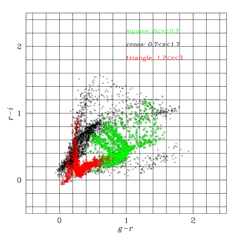
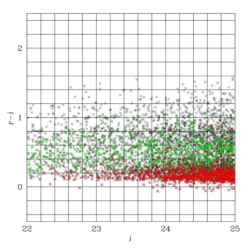
Figure 3 shows the distribution of galaxies in color space. Galaxies in three redshift intervals are shown to illustrate that, while they generally occupy different regions in color space, there is significant overlap, and moreover they cannot be isolated by making simple color cuts. We use these properties to guide our algorithm for selecting regions in color space for tomography in the next section.

Figure 4: The left panel shows the redshift distribution of four galaxy sub-samples using cuts in $r-i$ and $g-r$. The full sample is shown by the black lines. It is clear that the three sub-samples have overlap, but only at the $\sim 10\%$ level. The right panel shows the distributions obtained with more drastic cuts to better isolate the redshift sub-samples.

Figure 5: As in Figure 4, but for galaxies with $r<24$.

Figure 6: As in Figure 4, but using only $r-i$ color and $i$ magnitude to make the cuts. The left panel shows three sub-samples (with significant overlap) and the right panel two well separated sub-samples.

4 Color tomography with two and three-band imaging

4.1 Redshift sub-samples with color cuts

Having constructed our mock galaxy catalog, we used a set of heuristic criteria to cluster galaxies in color space. The goal is to construct 2-4 sub-samples with the “cleanest” possible redshift distributions. To achieve this we identify the redshift distribution of each region of color space, discard the regions with poorly behaved distributions, and group the rest into a set of sub-samples that would be useful for lensing tomography, i.e. have well separated and compact redshift distributions.

We pixelized $g-r$ vs. $r-i$ space into 400 pixels, and used the redshift distribution of each pixel to rank pixels in order of increasing mean redshift. We also characterized the compactness of the distribution associated with each pixel by computing its low order moments. We then grouped pixels into sub-samples following a set of heuristic criteria:

• The mean redshift associated with each pixel in a sub-sample fell within a well-defined redshift range.

• The redshift distribution of each pixel retained was sufficiently compact (had a small variance).

• The joint distribution of pixels included a desired fraction of the total number of galaxies (typically more than a quarter of the total).

• The mean redshifts of the 3 or 4 sub-samples were useful for lensing tomography, i.e. were sufficiently well spread out over the range $0.3\lower 2.15277pt\hbox{$\;\buildrel<\over{\sim}\;$}z\lower 2.15277pt\hbox{$\;\buildrel<\over{\sim}\;$}2.5$.

This was iterated to arrive at the final selection and grouping of color pixels and thus the boundaries of the final redshift sub-samples.

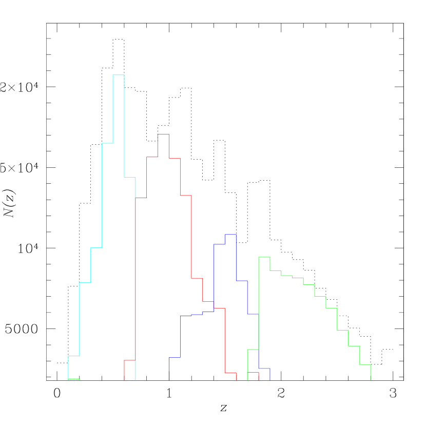
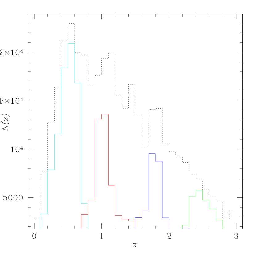
Figure 4 shows the results of making color cuts to isolate four redshift intervals with boundaries at $z=0,0.7,1.3,2.0,2.8$. We can trade-off number of galaxies within a sample versus how “clean” the redshift intervals are: the left and right panels of the figure show the results of different trade-offs. In the right panel, about half of the galaxies are discarded so that the resulting redshift samples have almost no overlap. In the left panel, the overlap is at the $10\%$ level or smaller. This level of overlap provides a clean enough separation for WL tomography, but risks contamination of the lensing signal by intrinsic alignments. Hence we use the more conservative choice in the right panel for dark energy forecasts below. We also note that for baryon oscillation measurements the widths in redshift of these sub-samples are too large; one would need to focus on finding particular galaxy types that yield tighter redshift distributions.

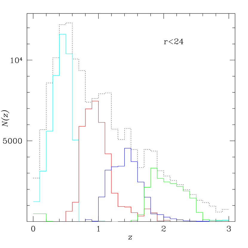
Figure 5 shows the results for a shallower sample with limiting magnitude $r=24$. The basic result is similar, though with fewer galaxies at $z>1$, it is more difficult to make four well separated sub-samples.

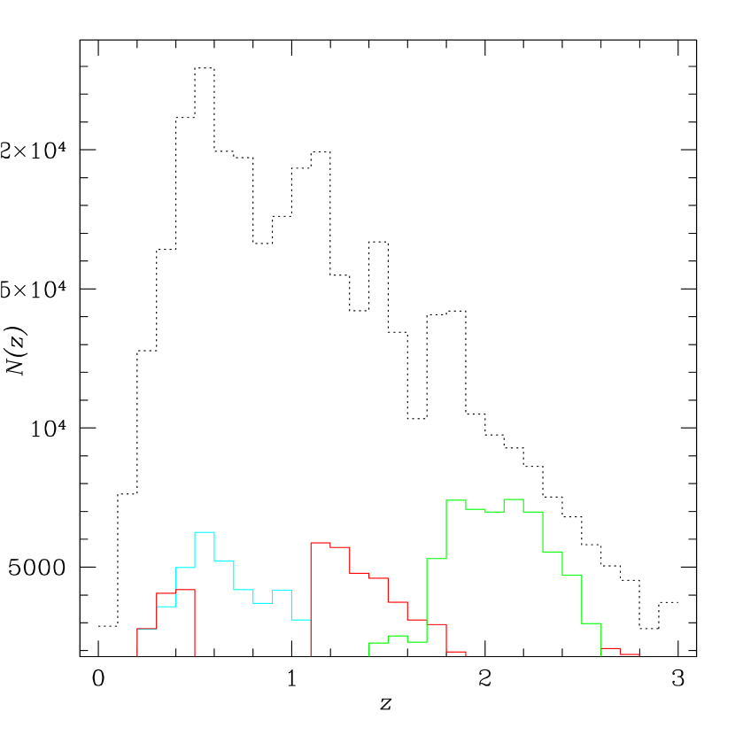
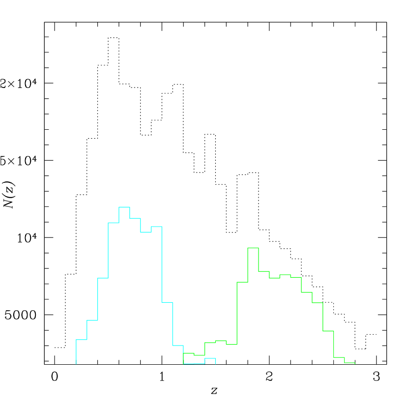
We also explored the possibility of lensing tomography with just two-band imaging. We used cuts in $r-i$ color and $i$ band magnitude to create two or three different redshift distributions (note that for the three-band case, we did not use the magnitudes to improve our redshift selection). While this is clearly an idealized exercise, in that it assumes a large calibration sample and does not include systematic errors or allow for variation in the spectral templates, the results in Figure 6 show that it is not a hopeless goal. Tomography is possible in up to three bins if $\sim 80\%$ of the galaxies can be discarded (left panel), though with significant overlap between the first two redshift samples. An alternative is to make just two samples (right panel) while losing fewer galaxies and having minimal overlap between the samples. We will quantify the consequences for cosmological parameter estimation below.

4.2 Lensing power spectra

Figure 7: Lensing power spectra $C(\ell)$ versus wavenumber $\ell$ from four redshift sub-samples, with boundaries at $z=0,0.7,1.3,2.0,2.8$. The error bars include sample variance and shot noise due to intrinsic ellipticity error for a $2,000$ square degree survey with $40$ galaxies per square arcminute. Note that the Fisher errors on dark energy parameters also include all the cross-spectra, which are not shown here.

Figure 8: Ratio of power spectrum errors with idealized photo-z’s and with color cuts. The power spectrum errors with photo-z’s assume that all galaxies within a given redshift range are used for the lensing power spectrum. The errors with color-cut are computed from the redshift distributions shown in Figure 4; these are larger as some fraction of galaxies have been discarded. The two panels use the distributions in the left and right panels in Figure 4 respectively; the colors of the symbols above match those of the distributions. The ratio of errors increase with $\ell$ since the relative contribution of the shot noise term to the error is larger at high $\ell$.

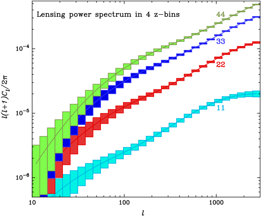
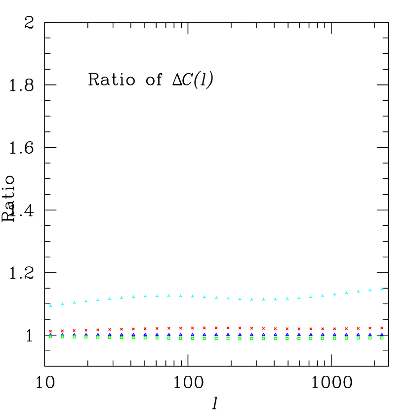
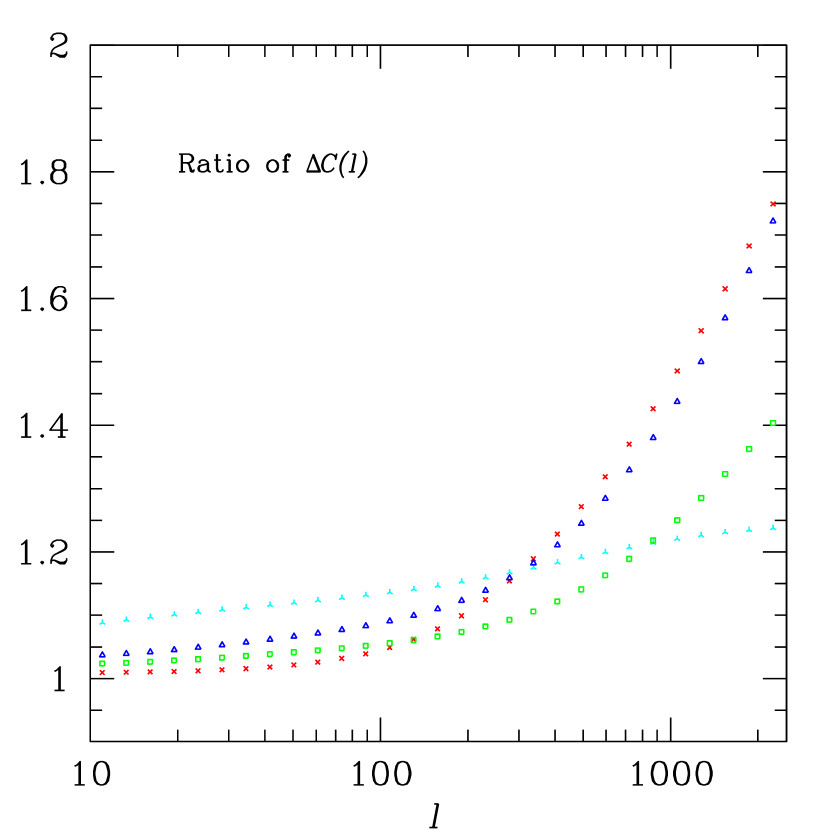
Figure 7 shows the lensing power spectra with errors for a 2,000 square degree survey with three-band imaging, using the four redshift distributions of Figure 4. Next we compare the errors on the power spectra for two cases: (a) All galaxies within a redshift range were used to compute the power spectrum (this represents the case of idealized photo-z’s), and, (b) Only galaxies selected using color cuts were used to compute the power spectrum (with distributions shown in the left panel of Figure 4). While the sample variance contribution is nearly the same as it depends on the amplitude of the power spectrum itself, the shot noise contribution is higher with the color cuts due to the loss in number density of galaxies.

Since the change in errors is undetectable on the power spectrum plot, we show the ratio of the errors for the two cases (idealized photo-z’s vs. color cuts) in Figure 8. The left and right panels correspond to the two sets of color cuts used in Figure 4. The errors increase by a few percent to over 50% depending on the sample and the range of $\ell$. At low wavenumber, $\ell\sim 100$, for all cases the increase in error is at the 10% level. Thus color tomography does not degrade the errors at low wavenumber, since the errors are dominated by sample variance. At high wavenumber $\ell\sim 1000$ the degradation depends on the fraction of galaxies discarded in making the redshift sample; for the right panel it is as high as 50%. The impact on dark energy parameters depends on the relative weights at low and high $\ell$. Note that we have underestimated the sample variance contribution to the errors by using only the Gaussian terms. The degradation due to the shot noise contribution would be smaller if non-Gaussian contributions to the sample variance were included (these are significant at $\ell\lower 2.15277pt\hbox{$\;\buildrel>\over{\sim}\;$}1000$).

4.3 Fisher analysis for cosmological parameters

Cosmological Parameters: Lensing

	Photo-z’s			3 bands/ 2 colors			2 bands/1 color
	6 $z$-bins		4 $z$-bins	4 $z$-bins∗		3 $z$-bins	2 $z$-bins
$\sigma(\Omega_{\rm de})$	0.019		0.023	0.027		0.048	0.1
$\sigma(w_{0})$	0.19		0.22	0.25		0.46	0.97
$\sigma(w_{a})$	0.64		0.72	0.86		1.4	2.6

Table 1: Summary of parameter constraints from lensing tomography using photo-z’s with 6 redshift bins (column 2); color cuts with three-band imaging to make 4 $z$-bins (column 3); and 4 $z$-bins with minimum overlap (denoted by ^∗, column 4); color cuts with two-band imaging to make 3 $z$-bins (column 5); and 2 $z$-bins with minimal overlap (column 6). All errors are $68\%$ confidence-level errors and include marginalization over the other parameters. Note that we have used $f_{\rm sky}=0.05$ and all the errors scale as $\propto f_{\rm sky}^{-1/2}$.

Cosmological Parameters: Lensing+CMB

	Photo-z’s			3 bands/ 2 colors			2 bands/1 color
	6 $z$-bins		4 $z$-bins	4 $z$-bins∗		3 $z$-bins	2 $z$-bins
$\sigma(\Omega_{\rm de})$	0.013		0.014	0.016		0.025	0.033
$\sigma(w_{0})$	0.11		0.13	0.15		0.24	0.32
$\sigma(w_{a})$	0.27		0.30	0.36		0.54	0.73

Table 2: Summary of parameter constraints from lensing tomography with CMB Planck priors. The columns are as in Table 1.

Having computed the lensing power spectra and the errors on them for different redshift samples, we estimate the errors on dark energy parameters using the Fisher matrix formalism. This formalism assesses how well given observables can distinguish the true (“fiducial”) cosmological model from other models. The parameter forecasts we obtain depend on the fiducial model and are also sensitive to the choice of free parameters. We include all the key parameters that may affect lensing observables within the CDM and dark energy cosmological framework: the density parameters are $\Omega_{\rm de}(=0.73)$, $\Omega_{\rm m}h^{2}(=0.14)$, and $\Omega_{\rm b}h^{2}(=0.024)$ (note that we assume a flat universe); the primordial power spectrum parameters are the spectral tilt, $n_{s}(=1)$, the running index, $\alpha_{s}(=0)$, and the normalization parameter of primordial curvature perturbation, $\delta_{\zeta}(=5.07\times 10^{-5})$ (the values in the parentheses denote the fiducial model). We employ the transfer function of matter perturbations, $T(k)$, with baryon oscillations smoothed out (Eisenstein & Hu 1999). The dark energy equation of state parameters are $w(a)=w_{0}+w_{a}(1-a)$, with fiducial values $w_{0}=-1$ and $w_{a}=0$.

Combining weak lensing with constraints from CMB temperature and polarization anisotropies can be a powerful way to lift parameter degeneracies (e.g. Hu & Tegmark 1999; Takada & Jain 2004). When computing the Fisher matrix for the CMB, we employ 9 parameters: the 8 parameters above plus the Thomson scattering optical depth to the last scattering surface, $\tau(=0.10)$. The Fisher matrix for the joint experiment is given by adding the CMB Fisher matrix to the lensing Fisher matrix as $F_{\alpha\beta}=F^{\rm WL}_{\alpha\beta}+F^{\rm CMB}_{\alpha\beta}$. We ignore the contribution to the CMB from the primordial gravitational waves. We use the publicly-available CMBFAST code (Seljak & Zaldarriaga, 1996) to compute the angular power spectra of temperature anisotropy, $C^{\rm TT}_{l}$, $E$-mode polarization, $C^{\rm EE}_{l}$, and their cross correlation, $C^{\rm TE}_{l}$. Specifically we consider the noise per pixel and the angular resolution of the Planck experiment that were assumed in Eisenstein et al. (1998). Note that we use the CMB information in the range of multipole $10\leq l\leq 2000$, and therefore we do not include the ISW effect at low multipoles $l\lower 2.15277pt\hbox{$\;\buildrel<\over{\sim}\;$}10$ which might be affected by dark energy perturbations.

4.4 Tomography with idealized photo-z’s versus color cuts

We compare the Fisher errors for lensing tomography with color cuts versus what is achievable with six redshift bins derived from an idealized set of photo-z’s using the LSST filter set. In both cases we ignore the scatter of galaxies across bins due to photometric errors and inexact spectral templates for galaxies. For color cuts, we consider three and two band imaging, and in each case we use two sets of redshift distributions to represent a more and less conservative treatment. These correspond to the right (more conservative) and left panels of Figures 4 (three band imaging) and 6 (two band imaging). We consider constraints from lensing alone as well as from lensing with CMB priors. We focus on dark energy parameters $w_{0}$ and $w_{a}$ but also comment on the errors on the primordial power spectrum.

Figure 9: Comparison of Fisher errors on dark energy parameters using “idealized photo-z” tomography (using all galaxies and 6 redshift bins - green ellipse) versus color tomography (blue ellipse). The color tomography ellipses are based on the four redshift sub-samples made with $g-r$ and $r-i$ cuts shown in the right panel of Figure 4 (the more conservative choice).

Figure 10: As in Figure 9, but including Planck priors for the CMB. This reduces the degradation for color tomography.

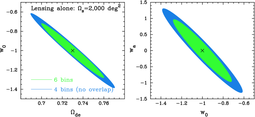
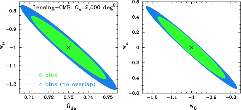
Figures 9 and 10 show the results for the dark energy parameters while Tables 1 and 2 give the numerical values of the errors on $\Omega_{\rm de}$, $w_{0}$, $w_{a}$. These are marginalized over all other parameters. Table 1 shows the constraints from lensing, while Table 2 includes the Fisher errors expected from CMB data from the Planck satellite. We have used only the lensing power spectrum; adding information from the lensing bispectrum or lensing-galaxy cross-correlations would improve the parameter constraints.

In Tables 1 and 2 the errors in column 2 (from 6 redshift bins with idealized photo-z’s) can be compared with columns 3 and 4 (4 $z$-bins using color cuts from three-band imaging data) and columns 5 and 6 (3 and 2 $z$-bins from two-band imaging). Columns 4 and 6 represent the conservative option for three and two-band imaging respectively, in that the redshift sub-samples have minimal overlap. For three-band imaging, even the conservative choice of column 4 shows that the degradation is modest: at the 30% level compared to the ideal case of 6-bin tomography. The loss of about half the galaxies does not prove very damaging as much of the cosmological information comes from the sample variance dominated regime. For two-band imaging, the degradation depends on whether one uses 3 or 2 $z$-bins. The last column shows that there is significant degradation with 2 $z$-bins. We found that even for this case, one parameter representing $w$ at the pivot redshift can be measured well. But constraints on $w_{0}$ and $w_{a}$ separately are severely compromised with just 2 $z$-bins.

The parameter degradations are significantly reduced when CMB information is used, as shown in Table 2. This is due to the coarser requirements of lensing tomography once the high-$z$ information from the CMB is used. Note that all these results depend on the lensing survey size, as the shot noise contribution affects parameter errors more for a smaller survey. And the results in Table 2 are less impressive if the CMB priors are from WMAP instead of Planck.

The constraints on the three dark energy parameters are shown in Figures 9 and 10. Idealized photo-z tomography is compared with 4 $z$-bin tomography from three-band imaging, using the more conservative choice of redshift sub-samples. These confirm the information in the tables: the degradation in the dark energy parameters is modest, and is even smaller in the best determined combination of $w_{0}$ and $w_{a}$, which is the value of $w$ at the pivot redshift for lensing.

We also note that lensing primarily probes parameters that are more sensitive to the lensing power spectrum amplitude rather than its shape parameters (see the discussion in Takada & Jain 2004). For our case these parameters are $\Omega_{\rm de}$, $w_{0}$, $w_{a}$ and $\delta_{\zeta}$. Adding redshift slices for tomography improves the errors on these parameters significantly up to 4-6 slices as it provides information on the redshift evolution of the amplitude of the lensing power spectrum. Errors on the shape parameters, such as the logarithmic slope of the power spectrum $n_{s}$, do not change appreciably.

5 Discussion

We have studied the prospects for lensing tomography with a wide area imaging survey that has limited color information. While it is never desirable to limit color information, it may be that a full complement of filters is not available at a survey telescope, that it is un-realistic to image the full survey area in all filters, or that additional science requirements for a survey dictate an observing strategy that is not optimal for lensing tomography. The questions we address in this study are whether lensing tomography is at all feasible with two or three band imaging data, and if so, what is the trade-off between filter choice and sky coverage.

We use the fact that lensing tomography makes only statistical use of estimated redshifts and, given the width of the lensing kernel, the redshift bins can be quite broad (though they must be known accurately). Further, for planned wide-area surveys lensing measurements are not shot noise limited – hence a significant fraction of galaxies can be discarded if their redshifts are ill-defined without severely degrading parameter accuracy. With these considerations in mind, we generate a mock catalog of galaxies extending to high redshift with known types, redshifts and colors. This provides an estimate of the redshift distributions for each part of $g-r$ and $r-i$ color space. From this we select regions in color space that produce sub-samples with redshift distributions well suited for tomography. Errors on the power spectra in different redshift bins from this color tomography are then compared with what would be expected with idealized photo-z’s.

The resulting degradation in the accuracy of cosmological parameters is shown in Tables 1 and 2, and Figures 9 and 10 for dark energy parameters from color tomography. With three-band imaging, the errors on dark energy parameters are only modestly degraded compared to idealized six-band photo-z’s. Even with two-band imaging, lensing tomography may be feasible for the case of high signal-to-noise data and an adequate calibration sample. This result may have implications for how to trade-off filter choice and sky coverage for large area surveys and how to optimize survey strategy to maximize the scientific returns in its initial stages. For example, imaging in three filters instead of six is more than twice as efficient in terms of survey time since the $u$ and $y$ filters (on the blue and red end) are substantially less efficient. Thus, for a fixed survey duration, the survey area for a six band program would be less than half that of the three band survey, with all parameter errors scaling as $f_{\rm sky}^{-1/2}$. Such trade-off studies must be carried out for the specific parameters and available choices in observing strategy for a given survey; the fiducial parameters we have considered do not correspond to any real or planned survey known to us.

For color tomography an adequate calibration sample is essential. The calibration will likely require a two-step approach: a sample of spectroscopic redshifts of over $\sim 10^{4}$ galaxies (for a $\sim 1000$ square degree survey), and a larger sample of multi-band imaging with a full set of optical and possibly infra-red filters. Imaging to a depth equivalent to $r\sim 25$ in say six bands over $10$-$20$ square degrees would provide a sample of well measured photo-z’s for over $1$ million galaxies. This would enable us to map the redshift distributions over the desired color space: e.g., it could provide photo-z’s of over $10^{4}$ galaxies in each bin of $\sim 0.1\times 0.1$ magnitude in two-colors (assumed to be available for the full survey area). It has been recognized that even with five or six band imaging data, photo-z’s would need to be carefully calibrated with spectroscopic redshifts so that the means and widths of redshift bins are known to high accuracy (Bernstein & Jain 2004; Huterer et al. 2006; Ma, Hu and Huterer 2006), and proposals for calibration are being developed (Newman 2006). For color tomography the calibration sample is even more important, as it forms the basis for grouping and discarding regions in color space. We leave for future work the detailed requirements and strategy for obtaining the calibration sample.

Our current study is based on estimates of statistical errors in the lensing power spectra – in future work we will include systematic photometric uncertainties and other systematic errors that affect lensing. These will include a realistic modeling of photometric errors, filter design, and will address whether the spectral templates are adequate for describing high-redshift galaxies. The inclusion of these realistic errors is essential before one can make detailed trade-off studies of survey duration and filter choice. Several caveats are in order until such a study is done: systematic errors may lower the signal-to-noise and this may depend on scale, testing for systematics is more difficult with coarser redshift bins, and marginalizing over intrinsic ellipticity contributions may be harder (see below). Finally, the inclusion of other statistics such as higher order correlations and cross-correlations with the galaxy distribution can alter the results on parameter accuracies. Some of these issues can be tested on ongoing multicolor surveys, such as the CFHT Legacy Survey.

Our results on the power spectrum errors in Figure 8 show that the degradation in errors is worse at high $\ell$, because the shot noise term dominates on small scales. This raises the question: should one choose different galaxy samples at different $\ell$: be more conservative at low $\ell$, since number density matters less, to minimize redshift overlap and bias? This merits a detailed study as it has the potential to impact different survey strategies. Such a study must include non-Gaussian contributions that increase the sample variance at high $\ell$; this in fact lowers the degradation for color tomography as the shot noise regime shifts to higher $\ell$ (e.g. Kilbinger & Schneider 2005).

Finally, intrinsic ellipticity alignments (e.g. Heymans et al. 2006) and ellipticity-shear alignments (Hirata & Seljak 2004) must be considered. While we did choose as our fiducial sub-samples ones with well separated redshift distributions, it may be necessary to only use cross-spectra to eliminate intrinsic ellipticity contributions (e.g. Takada & White 2004). This would increase the parameter errors from having a smaller number of redshift bins. Similarly ellipticity-shear correlations may need to be measured from the data and marginalized over, which is easier to do with finer redshift binning. Four redshift bins are the minimum needed to separately fit for both kinds of intrinsic ellipticity correlations, this may impose a minimal requirement on the needed color information. The impact of intrinsic alignments is likely to be the most important issue for future studies related to color tomography.

References

- Connolly et al. (1995) Connolly, A., Csabai, I., Szalay, A.S., Koo, D., Kron, R.G., Munn, J.A., 1995, AJ, 110, 2655
- Connolly et al. (2002) Connolly, A., et al., 2002, ApJ, 579, 48.
- Eeisenstein & Hu (1999) Eisenstein, D., Hu, W., 1999, ApJ, 511, 5
- Eisenstein, Hu & Tegmark (1998) Eisenstein, D., Hu, W., Tegmark, M., 1998, ApJ, 518, 2
- Franceschini et al. (2006) Franceschini, A., et al. 2006, A&A, 453, 397
- Heymans et al. (2006) Heymans, C., White, M., Heavens, A., Vale, C., & Van Waerbeke, L. 2006, MNRAS, 817
- Hirata & Seljak (2004) Hirata, C. M., & Seljak, U. 2004, Phys. Rev. D, 70, 063526
- Hoekstra et al. (2005) Hoekstra, H. et al., 2005, ApJ (submitted), astro-ph/0511089
- Hu (1999) Hu, W., 1999, ApJ, 522, L21
- Hu & Tegmark (1999) Hu, W., & Tegmark, M. 999, ApJ, 514, L65
- Hu (2002) Hu, W., 2002, Phys. Rev. D66, 083515
- Huterer & Takada (2005) Huterer, T., Takada, M., 2005, Astropart. Phys., 23, 4
- Huterer et al. (2006) Huterer, D., Takada, M., Bernstein, G., & Jain, B., 2006, MNRAS, 366, 101
- Jain & Seljak (1997) Jain, B., Seljak, U., 1997, ApJ, 484, 560
- Jain, Jarvis & Bernstein (2005) Jain, B., Jarvis, M., & Bernstein, G. 2006, JCAP, 02, 001
- Jarvis et al. (2003) Jarvis, M., et al., 2003, AJ, 125, 1014
- Jarvis et al. (2005) Jarvis, M., Jain, B., Bernstein, G., Dolney, D., 2006, ApJ, 644, 71
- Kilbinger & Schneider (2005) Kilbinger, M., & Schneider, P. 2005, A&A, 442, 69
- Linder & White (2005) Linder, E. V., & White, M. 2005, Phys. Rev. D, 72, 061304
- Ma, Huterer, & Hu (2006) Ma, Z., Hu, W. & Huterer, D., 2006, ApJ, 636, 21
- Metcalfe et al. (2001) Metcalfe, N., Shanks, T., Campos, A., McCracken, H. J., & Fong, R. 2001, MNRAS, 323, 795
- Newman (2006) Newman, J., 2006, private communication
- Perlmutter et al. (1999) Perlmutter, S., et al., 1999, ApJ, 517, 565
- Riess et al. (1998) Riess, A., et al., 1998, AJ, 116, 1009
- Schneider et al. (2006) Schneider, M., et al 2006, Ap J, submitted, arXiv:astro-ph/0606098
- Seljak & Zaldarriaga (1996) Seljak, U., Zaldarriaga, M., 1996, ApJ, 469, 437
- Spergel et al. (2006) Spergel, D. N., et al. 2006, arXiv:astro-ph/0603449
- Takada (2006) Takada, M., 2006, Phys. Rev. D, 74, 043505
- Takada & Jain (2004) Takada, M., Jain, B., 2004, MNRAS, 348, 897
- Takada & White (2004) Takada, M., White, M., 2004, ApJ, 601, L1
- White & Vale (2004) White, M., Vale, C., 2004, Astropart. Phys. 22, 19
- Zhan & Knox (2006) Zhan, H., & Knox, L. 2006, ApJ, 644, 663
- Willmer et al. (2006) Willmer, C. N. A., et al. 2006, ApJ, 647, 853