Sun-as-a-star observations: evidence for degree dependence of changes in damping of low-$\ell$ p modes along the solar cycle

Abstract

Aims. We use 9.5-yr of BiSON Sun-as-a-star data to search for dependence of solar-cycle parameter changes on the angular degree, $\ell$, of the data. The nature of the Sun-as-a-star observations is such that for changes measured at fixed frequency, or for changes averaged across the same range in frequency, any $\ell$ dependence present carries information on the latitudinal distribution of the agent (i.e., the activity) responsible for those changes.

Methods. We split the 9.5-yr timeseries into contiguous 108-d pieces, and determine mean changes in the damping of, power in, and energy supplied to the modes through the solar cycle. We also apply a careful correction to account for the deleterious effects of the ground-based BiSON window function on the results.

Results. From our full analysis we obtain a marginally significant result for the damping parameter, where the mean change is found to be weakest at $\ell=0$. The other parameters show hints of some dependence in $\ell$.

Conclusions. Our main conclusion is that the mean fractional solar-cycle change in the $\ell=0$ damping rates is approximately 50 % smaller than was previously assumed. It had been common practice to use an average over all low-$\ell$ modes; our downward revision of the radial-mode value has implications for comparisons with models of the global solar cycle changes, which are usually based on a spherically symmetric geometry.

1 Introduction

The fact that damping rates and powers of the global p modes change through the solar cycle is now well established (e.g., Chaplin et al., 2000; Komm et al., 2000; Salabert et al., 2003; Jiménez-Reyes et al., 2003, 2004; Salabert & Jiménez-Reyes, 2006). At least where the main part of the p-mode spectrum is concerned damping gets heavier, and observed power gets weaker, as the level of solar activity increases. Information on the damping and power parameters comes straightforwardly from the observations. The damping rates are assumed to be linearly related to the linewidths of the resonant peaks in the frequency power spectrum; while the powers are proportional to the product of the peak widths and heights (the latter more formally termed the maximum power spectral densities).

Komm et al. (2002) took advantage of the large number of components available to analyze in the medium-degree range (from $\ell=40$ to 80) the latitudinal dependence of the width and height changes. They found that the changes were concentrated in latitudes occupied by the active regions. The damping rates and powers, like the mode frequencies, therefore seemed to be responding in some fashion to changes wrought on the active regions by the changing magnetic fields.

Most of the low-$\ell$ results have come from the Sun-as-a-star data (e.g., from BiSON, GOLF, IRIS and VIRGO/SPM; or from GONG and MDI data combined into a Sun-as-a-star-like proxy). These data show only the even $\ell+m$ components; the odd components are so weak as to be unobservable. Since it is the outer, sectoral components (with $\ell=|m|$) that appear most prominently, the Sun-as-a-star mode parameters estimated by the usual analysis methods are dominated by, and therefore close to, the sectoral values. This characteristic gives a noticeable change in the latitudinal sensitivity from $\ell=0$ to $\ell=1$, 2 or 3. The spatial sensitivity of Sun-as-a-star data at the latter three values of $\ell$ is weighted toward the lower latitudes, where the active regions reside. The Sun-as-a-star parameters at these $\ell$ are therefore more sensitive to the solar cycle than are the $\ell=0$ data. Evidence for $\ell$ dependence in the shifts of the Sun-as-a-star mode parameters therefore carries information on the latitudinal distribution of the agent responsible for those shifts. (Changes in inertia, at fixed frequency, between these $\ell$ are very small indeed.)

It is much more difficult to uncover spatial dependence of the mode parameter changes in the low- than in the medium-$\ell$ data because there are far fewer components to analyze, and uncertainties on the results are commensurately larger. When changes to damping and power were first uncovered in the Sun-as-a-star data, results were averaged over $\ell$ to reduce errors. Given the modest precision in the results, it was assumed the $\ell$-averaged values also provided a working proxy of the radial-mode shifts. And so these averages were used as meaningful comparisons for models of global changes in damping (see, e.g., Houdek et al., 2001), models set up in spherical geometry, i.e., pertinent only to the $\ell=0$ case. With better analysis, and more data, it has become possible to give results for each $\ell$, and to therefore test whether the $\ell=0$ shifts really are weaker than an average across $\ell=0$ to 2 or 3.

We made a first cut at such an analysis in Chaplin et al. (2003a). Our results, from BiSON Sun-as-a-star data, suggested very strongly that the $\ell=0$ linewidth changes were indeed significantly weaker than at $\ell=1$ and 2. The clear implication was that results of the theoretical models would now need to be compared to this new, smaller shift. In the analysis of the BiSON data, we had to allow for the corrupting influence on the results of the ground-based BiSON window function. We did so by applying corrections that were designed originally for a different study, using data from a different period. In this paper we revisit our analysis. We design and implement a correction procedure for the 9.5-yr BiSON dataset in question. We find that implementation of this internally consistent, and more accurate, correction gives little change to the results, and reinforces our earlier conclusion. In summary, the mean fractional solar-cycle change in the $\ell=0$ damping rates is approximately 50 % smaller than was previously assumed.

2 Data analysis

2.1 Observations

Our analysis made use of 3456 d of data on the low-angular-degree solar p-modes, collected by the six-station, ground-based Birmingham Solar-Oscillations Network (BiSON). This 9.5-yr dataset had a starting date of 1992 July 26, and spanned the falling phase of solar cycle 22 and the rising phase, and the maximum, of solar cycle 23.

The instruments at each BiSON site make Sun-as-a-star observations of the Doppler shift of the potassium Fraunhofer line at 770 nm (e.g., Chaplin et al., 1996). Raw data were first processed in the manner described by Elsworth et al. (1995) to yield daily calibrated velocity residuals. We then combined coherently the resulting $\approx 2\times 10^{4}$ individual daily sets from all six stations to yield the principal 3456-d time series of residuals. The duty cycle of this combined set was $\sim 76$ %, with breaks in coverage largely the result of inclement weather.

In order to derive solar-cycle trends, the 3456-d series was divided in thirty-two contiguous, independent 108-day pieces, which had a range of duty cycles between 63 and 87 per cent. This 108-d interval, a multiple of the solar rotation period, was chosen to minimize effects dependent on the solar rotation.

2.2 Mode parameter extraction

The power spectrum of each 108-day time series was fitted to yield estimates of the mode parameters over a range in frequency $1600\leq\nu\leq 3800\,\rm\mu Hz$. This fitting was done by a multi-step iterative method based on Gelly et al. (2002). The asymmetric profile of Nigam & Kosovichev (1998) was used to describe each component, as:

$$\mathcal{M}(x)=H\frac{(1+bx)^{2}+b^{2}}{1+x^{2}},$$ (1)

where $x=2(\nu-\nu_{0})/\Gamma$, and $H$, $\Gamma$, $\nu_{0}$ are the mode height (maximum power spectral density), the fwhm linewidth, and the central frequency respectively. The parameter $b$ is the asymmetry coefficient, which in the present analysis was fixed at small negative values determined by analysis of longer datasets.

Due to their close proximity in frequency, modes were fitted in pairs (i.e., $\ell=2$ with 0 and $\ell=3$ with 1). An additional offset was included in the fitting model to describe the background level in the fitting window. The first temporal sidebands at $11.57\,\rm\mu Hz$ were also included in the model. The mode parameters were extracted by maximizing a likelihood function commensurate with the $\chi^{2}$, 2 degrees-of-freedom statistics of the power spectrum. The natural logarithm of the height, width and background terms were varied – not the parameter values themselves – in order to give quasi-normal fitting distributions. Formal uncertainties on the fitted values were then derived from the Hessian matrix of each fit in the usual manner.

2.3 Damping and excitation parameters

A generally accepted analogy for the p modes is a forced and damped harmonic oscillator. For any given mode ($n,\ell$), the mode width, $\Gamma_{n,\ell}$, is then linearly related to its damping rate, $\eta_{n,\ell}$. The total velocity power, $P_{n,\ell}$, gives a measure of the balance between the excitation and damping, and is proportional to the product of the height, $H_{n,\ell}$, and the mode width, $\Gamma_{n,\ell}$. The rate at which the energy is supplied to the modes, $\dot{E}_{n,\ell}$, is a direct measure of the net forcing and is independent of the mode damping. This ‘supply rate’ can be computed as the product of the mode width, $\Gamma_{n,\ell}$, and the mode energy, $E_{n,\ell}$, the mode energy being proportional to the mode power, $P_{n,\ell}$. For a detailed description of the mode damping and excitation parameters, see, e.g., Chaplin et al. (2000).

Since the peak-finding procedure returned natural logarithms of the mode heights and widths, estimates of the mode velocity power and supply rate were made by taking the combinations:

$$\log_{e}(P_{n,\ell})=\log_{e}(H_{n,\ell})+\log_{e}(\Gamma_{n,\ell})+\rm{c_{1}},$$ (2)

and

$$\log_{e}(\dot{E}_{n,\ell})=\log_{e}(H_{n,\ell})+2\log_{e}(\Gamma_{n,\ell})+\rm c{{}_{2}}.$$ (3)

Variations in the fitted logarithmic parameters therefore corresponded to fractional variations of the absolute parameters. The factors $\rm{c_{1}}$ and $\rm c{{}_{2}}$ in the above contain information on the mode inertia, and mode visibility given by the instrument. The factors were assumed to remain unchanged over the epoch in question, and were therefore ignored in the solar-cycle analysis. Uncertainties on the mode velocity power and on the mode energy supply rate were determined by taking into account the strong anti-correlation between the extracted mode heights and mode widths (Chaplin et al., 2000).

Hereafter, we write the natural logarithm of $H_{n,\ell}$, $\Gamma_{n,\ell}$, $P_{n,\ell}$, and $\dot{E}_{n,\ell}$ as $h_{n,\ell}$, $\gamma_{n,\ell}$, $p_{n,\ell}$, and $\dot{e}_{n,\ell}$ respectively.

2.4 Determination of the fractional variations

Estimates of the fractional variations of the mode parameters over time were obtained by performing a linear regression of each of the fitted parameters $\gamma_{n,\ell}$, $p_{n,\ell}$, and $\dot{e}_{n,\ell}$, on the 10.7-cm solar radio flux ($F_{10.7}$). The radio flux was used as a robust proxy of the global level of solar activity. The best-fitting gradients therefore gave for each mode a measure of sensitivity of its parameters to the solar activity.

The regressions were computed as both un-weighted and weighted linear fits. The formal parameter uncertainties from the mode-fitting procedures, derived from the Hessian matrices of the fits, were used here to compute weights for weighted linear regressions. Fitted gradients from the regressions were then averaged at each degree over the frequency range between 2600 $\mu$Hz and 3600 $\mu$Hz. This averaging yielded estimates of mean mode changes along the cycle.

There are different ways to compute these averages and their associated uncertainties. On the one hand, a simple, unweighted mean of the input residuals may be calculated, with the scatter on the residuals used to determine the uncertainty on the mean (in the usual manner). An alternative is to use the Hessian-determined uncertainties on the best-fitting gradients to calculate weighted means. The error on the mean can then be estimated in one of two ways: first, from a suitable combination of the Hessian-determined uncertainties, giving an internal error; and second, by using the Hessian-determined uncertainties to weight a calculation of the dispersion of the data, giving an external error (Chaplin et al., 1998).

Since the regression fits were performed in two ways (un-weighted and weighted) there are six ways in all to estimate the degree dependence of the p-mode damping and excitation parameters, and the associated uncertainties (although the weighted-average methods of course give the same means, but have different errors).

3 Correction for bias

Gaps present in the timeseries of a ground-based window function lead to overestimation of the mode widths and underestimation of the mode heights (Chaplin et al., 2003b). Proper allowance must therefore be made for any bias introduced by the window functions of the thirty-two 108-d BiSON timeseries. Furthermore, marked changes in the intrinsic quality of the data can in principle influence the parameters, via the impact changes in quality may have on the observed height-to-background ratios of the mode peaks. Changes in height-to-background ratio must, however, be large to give any significant bias in the parameters.

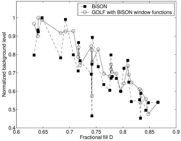
We have used Monte Carlo simulations of artificial Sun-as-a-star data to help us correct the BiSON results for bias introduced by these effects. We found that the bias was dominated by the impact of the different 108-d window functions; the impact of changes in data quality was far less significant. The domination of the window function is illustrated in Fig. 1. It shows the mean background levels, of the thirty-two 108-d BiSON, spectra over the range 2600 to $3600\,\rm\mu Hz$ (-$\blacksquare$-). The values have been scaled so that the highest mean background level is set to unity. The levels are plotted as a function of the duty cycle, $D$, of each of the sets. As fill decreases, the redistribution of power by the window function increases the background level.

Also shown in Fig. 1 are results for a single, 108-d GOLF timeseries. The GOLF timeseries has nearly a 100 % duty cycle, and has been modulated, in turn, by each of the thirty-two BiSON window functions. The resulting mean background levels have been plotted (-$\circ$-). Because the GOLF data are the same for each computation, the change in the background level comes wholly from the impact of the window function. Changes to the background in these modulated GOLF data are seen to follow very closely the changes observed in the BiSON data. From this, we conclude the window function dominates changes to the background. The result simplifies the generation of artificial data for the Monte Carlo simulations in that we do not need to worry about introducing changes in intrinsic data quality across the simulated datasets.

Figure 1: Normalized background level for the thirty-two 108-d BiSON spectra (-$\blacksquare$-) and the single 108-d GOLF set modulated in turn by each of the BiSON window functions (-$\circ$-). Background levels are averaged over 2600 and 3600 $\mu$Hz, and normalized so that the highest datum takes the value unity. Data are plotted as a function of the duty cycle, $D$.

3.1 Bias estimation from artificial Sun-as-a-star data

The artificial data were generated using the solarFLAG (Chaplin et al., 2006) mode simulation code. The Laplace transform solution of the equation of a forced, damped harmonic oscillator was used to generate each component at a 40-s cadence in the time domain, in the manner described by Chaplin et al. (1997). Components were re-excited independently at each sample with small ‘kicks’ drawn from a Gaussian distribution. The model gave rise to peaks in the frequency power spectrum whose underlying shapes were Lorentzian. It should be pointed out that the observed low-$\ell$ peaks are slightly asymmetric in shape (albeit at the level of only a few per cent at most).

Datasets were constructed component by component in the time domain. Sets were made with a full cohort of simulated low-$\ell$ modes, covering the ranges $0\leq\ell\leq 5$ and $1000\leq\nu\leq 5500\,\rm\mu Hz$. A database of mode frequency, power and linewidth estimates, obtained from analyses of GOLF and BiSON data, was used to guide the choice of input values for time-series construction. A rotational frequency splitting of $0.4\,\rm\mu Hz$ was imposed on all the non-radial modes, irrespective of overtone number and angular degree, to match that extracted from observations. A ‘pink’ background noise component was also added in the time domain, the size of which increased at lower frequencies in order to give signal-to-background ratios commensurate with GOLF or BiSON-like Doppler velocity data.

Two cohorts of data were made, both comprising twenty 3456-d timeseries. Each timeseries was excited with independent realization noise. We introduced into the first cohort (# 1) systematic changes in the frequency, damping and power parameters so as to simulate the effects of the solar cycle (see Chaplin et al., 2006). These changes were based on variations of a modelled proxy of the 10.7-cm radio flux. The proxy was made to mimic the radio flux for the real epoch covered by the BiSON timeseries. Parameter variations were calibrated to give equal, and oppositely directed, changes in the damping and power parameters (i.e., $\delta\gamma_{n,\ell}=\delta p_{n,\ell}$), to match previous observations (e.g., Chaplin et al., 2000). In this scenario the supply rate, $\dot{e}_{n,\ell}$, shows no net change. The simulated changes were frequency dependent, showing their largest variations at 2900 $\mu$Hz. Furthermore, they were given no $\ell$ dependence. In contrast, in the second ‘stationary’ cohort (# 2) all mode parameters were held constant in simulated time.

We analyzed each artificial 3456-d dataset in the manner described in Sections 2.2 and 2.4, the first step being to split them into 108-d pieces. From the analysis, we obtained $\ell$-dependent estimates of mean changes in the $\gamma_{n,\ell}$, $p_{n,\ell}$, and $\dot{e}_{n,\ell}$ parameters. Results from all 3456-d sets were then averaged within their respective cohort to reduce errors. Final estimates of the mean parameter changes could then be compared with the true changes introduced, to allow for a determination of the bias.

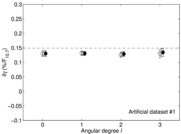
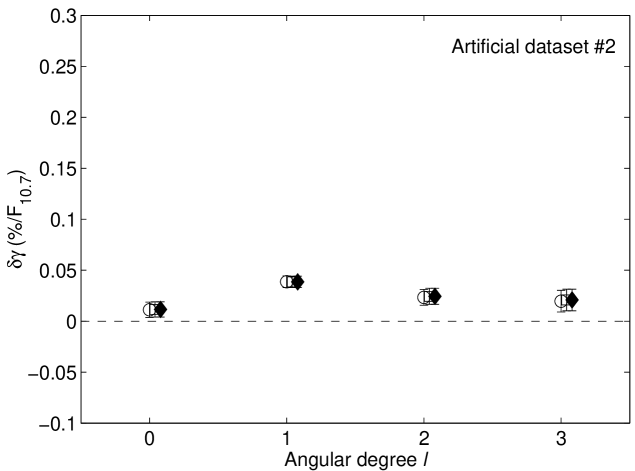
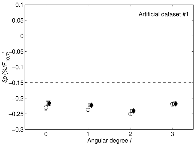
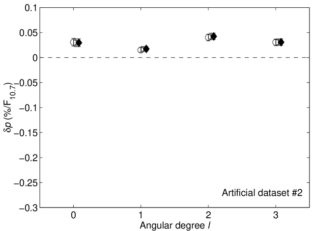
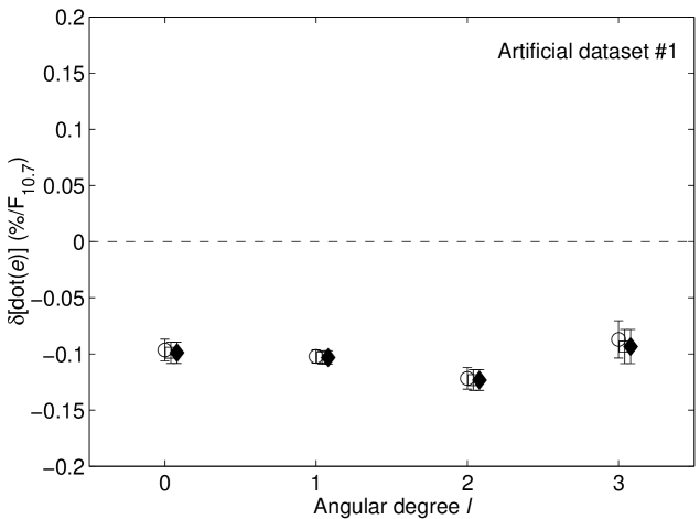
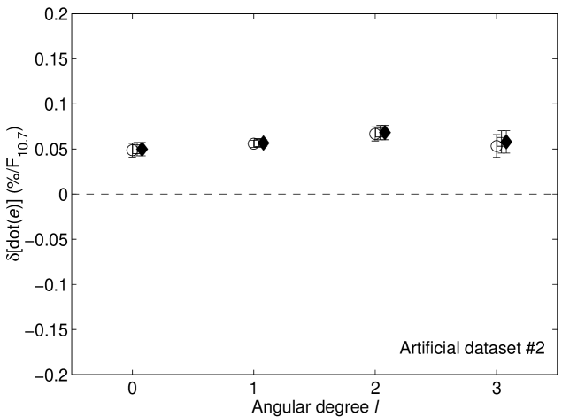
Similar mean values and errors were returned by the different averaging methods (Section 2.4). For the sake of clarity we show in what follows results from the weighted regressions only. The three panels in the left-hand column of Fig. 2 show the mean estimated parameter variations, per unit change in the radio flux, given by analysis of artificial cohort # 1 (the ‘solar-cycle’ data). The right-hand panels show results from cohort # 2 (the ‘stationary’ data). The horizontal dashed lines show the actual mean changes that were introduced in the artificial parameters. The plotted uncertainties in each panel show the error bars on the mean results of the twenty artificial datasets.

The results in Fig. 2 show evidence for both overestimation and underestimation of input values, dependent on the parameter and cohort. Bias is most severe in the determination of the change in power and supply rate in cohort # 1. In spite of the offsets, it is encouraging to note that there is no appreciable variation of the bias with degree. Any variation would certainly be well within the uncertainties expected from analysis of a single, 3456-d dataset (which are a factor $\sqrt{20}$ larger than the errors plotted in Fig. 2).

From these artificial data we then went on to derive a window-function parameter correction that could be applied to the real BiSON observations. Because of the small errors on the artificial data results, the correction would be well constrained, and uncertainties on the results in Fig. 2 would therefore not add significantly to the uncertainties on the final, corrected BiSON results.

3.2 Formulation of correction procedure

The following procedure was applied to the fitted parameters within each cohort of artificial data.

We began by computing the ratio of the fitted and input parameters of every fitted mode. Ratios were made for the heights, $h$, and widths, $\gamma$. Recall that each of the twenty independent 3456-d sets was split into thirty-two 108-d pieces for fitting. We therefore obtained many ratios, $Q_{h}(i,j,n,\ell)$ and $Q_{\gamma}(i,j,n,\ell)$. The variable $i$ ran over the independent sets ($1\leq i\leq 20$); while $j$ ran over the 108-d pieces ($1\leq j\leq 32$), each having their own distinct BiSON window function.

Next, we averaged the ratios over the twenty independent datasets (over $i$). This gave a total of thirty-two mean parameter ratios for every mode, one for each 108-d window function. These mean parameter ratios, $Q(j,n,\ell)$, were then regressed linearly against the duty cycles, $D(i)$, of each of the windows; in fact, we fitted to $1-D(i)$, rather than $D(i)$. The fits gave best-fitting gradients $\delta Q^{\rm D}(n,\ell)$.

By following the above procedure for each cohort of artificial data, we obtained two sets of mean ratios and best-fitting gradients. We were then in a position to construct, from the ratios and gradients, a formalism for correcting the fitted BiSON parameters for the window function. In short, it would allow us to make estimates of the unbiased parameters by linear extrapolation to $D=1.0$.

First, we checked the procedure could be applied to the fitted artificial mode parameters to recover correct estimates of the mean input changes in cohorts # 1 and # 2. This would involve performing a full analysis on each of the artificial 3456-d sets, and would be a dry run of the full correction and analysis as it would be applied to real BiSON data. Taking the width parameter as an example, estimates of the unbiased widths, $\gamma_{Q}(j,n,\ell)$, were given by the linear combination:

$$\gamma_{Q}(j,n,\ell)=\gamma(j,n,\ell)\times\{Q_{\gamma}(j,n,\ell)+[1-D(i)]\times\delta Q^{\rm D}_{\gamma}(n,\ell)\}^{-1}.$$ (4)

A similar equation was used to define a correction for the mode heights. Once we had obtained estimates of the unbiased widths (and heights) from Equation 4 (and its mode-height counterpart), the corrected parameters were then used to estimate mean parameter variations. We used the corrected parameters as input to the analysis outlined in Section 2.4, and found we were able to recover, within errors, the input cycle shifts when we analyzed datasets from cohort # 1; and the expected null changes when we analyzed datasets from cohort # 2. To illustrate the success of the correction procedure, Table 1 shows the linear correlation between the estimated and input width changes for sets in cohort # 1 before (top row) and after (bottom row) the correction was used. Given the numbers of data involved, these represent significant improvements in the correlation, and the final result.

Figure 2: Results of analysis of artificial data. Shown are mean fractional variations (% per unit of change in $F_{10.7}$) in mode damping, $\delta\gamma$ (upper panels), mode velocity power, $\delta p$ (middle panels), and mode energy supply rate, $\delta\dot{e}$ (lower panels), as a function of the mode angular degree $\ell$. Panels in the left-hand column show results averaged over the twenty artificial 3456-d sets in cohort # 1; those in the right-hand column similar averages over sets in cohort # 2. The dashed lines in each plot represent the modelled, input changes. The symbols give information on how the averages were computed (see Sec. 2.4): unweighted mean -$\circ$-; weighted mean with internal error -$\square$-; weighted mean with external error -$\blacklozenge$-. Plotted errors are those on the mean of the twenty artificial datasets.

Table 1: Linear correlations between the fractional variations in mode width (% per unit of change in $F_{10.7}$) extracted from the artificial datasets in cohort# 1 and the true, input variations without and with temporal window function corrections (Equation 4).

$\delta\gamma$	$\ell=0$	$\ell=1$	$\ell=2$	$\ell=3$
No correction	0.80	0.93	0.96	0.61
With correction	0.98	0.99	0.99	0.94

4 Results with Sun-as-a-star BiSON data

With the correction checked on the artificial data, we proceeded to apply the procedure to fitted parameters from the thirty-two 108-d BiSON datasets. We used the mean parameter ratios, $Q(j,n,\ell)$, and the best-fitting gradients, $\delta Q^{\rm D}(n,\ell)$, from the artificial data. Recall there were two sets of these coefficients: one from artificial cohort # 1, the other from artificial cohort # 2. The window-function correction procedure was therefore applied twice, yielding two sets of corrected parameters.

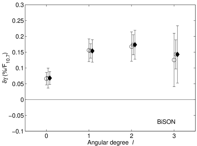
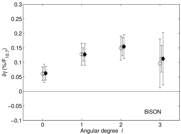
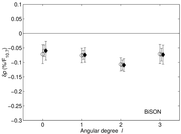
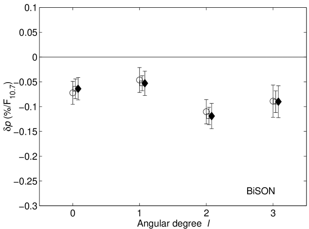
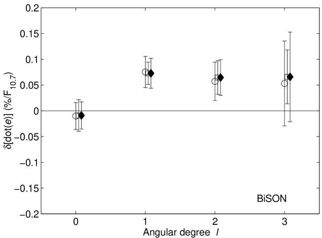
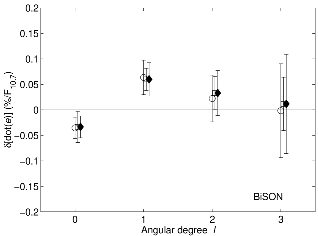
Estimates of the unbiased height and width parameters were then analyzed, as per Section 2.4. This give the sought-for estimates of the mean parameter changes, per unit change in the radio flux. Again, these changes – which are shown in Fig. 3 – represent averages for each $\ell$ over the range 2600 to $3600\,\rm\mu Hz$. The plots in the left-hand column show results given by the cohort # 1 correction coefficients; those in the right-hand panels results given by the cohort # 2 coefficients. The results are also summarized in Table 2. Here, we have multiplied the shift-per-unit-activity values shown in Fig. 3 (the external mean data -$\blacklozenge$-) by the change in the radio flux observed across the thirty-two 108-d pieces, to give estimates of the mean parameter changes over the solar cycle.

We found good agreement, to within the errors, between results given by the cohort # 1 and # 2 corrections. Averages made over the $l=0$, 1 and 2 results were in reasonable agreement with previous analyses of the BiSON, IRIS and GOLF Sun-as-a-star data (Chaplin et al., 2000; Salabert et al., 2003; Jiménez-Reyes et al., 2003, 2004). However, the most striking feature of Fig. 3 is the apparent relative weakness of changes in the $\ell=0$ widths, implying an $\ell$ dependence of the results. Inspection of results for the power parameter showed hints of a mirrored, albeit weaker, trend. There were also indications of a jump in $\ell$ in the supply-rate results (in particular for the cohort # 1 corrected data).

To ascribe some formal significance to the weakness of the $\ell=0$ width shift, we first compared its value with the weighted mean of the $\ell=1$ and 2 width shifts (we ignored the less-well-constrained $\ell=3$ data). The $\ell=0$ value was found to be about $2\sigma$ different from the mean over $\ell=1$ and 2, for both cohort corrections. However, when we computed a linear regression of the mean shifts on $\ell$, we found gradients $\approx 3\sigma$ and $\approx 4\sigma$ different from zero for the cohort # 1 and cohort # 2 coefficients respectively. We conclude that there is marginally significant evidence for an $\ell$ dependence of the width changes. Similar analysis of the other parameters gave weaker levels of correlation, and therefore showed no evidence for significant variation, with $\ell$. Whether the hint of variation in the power and supply rate results is real only more data, and independent confirmation from other observations (e.g., GOLF) will tell.

Figure 3: Results of analysis of BiSON data. Shown are mean fractional variations (% per unit of change in $F_{10.7}$) in mode damping, $\delta\gamma$ (upper panels), mode velocity power, $\delta p$ (middle panels), and mode energy supply rate, $\delta\dot{e}$ (lower panels), as a function of the mode angular degree $\ell$. Panels in the left-hand column show results given using the cohort # 1 coefficients in the window-function correction; those in the right-hand column results from using the coefficients from cohort # 2. The solid horizontal lines in each plot mark the zero-change level for reference. The symbols give information on how the averages were computed (see Sec. 2.4): unweighted mean -$\circ$-; weighted mean with internal error -$\square$-; weighted mean with external error -$\blacklozenge$-.

Table 2: Fractional variations (%) of the low-degree p-mode damping and excitation parameters from solar minimum to solar maximum for each $\ell$ value, averaged over 2600 and 3600 $\mu$Hz. Final results are shown for application of the window-function correction coefficients from artificial data cohorts # 1 and # 2 (see Sec. 3.2). Data correspond to the external mean shifts, rendered as -$\blacklozenge$- symbols in Fig. 3.

Parameter	$\ell=0$	$\ell=1$	$\ell=2$	$\ell=3$	$\left<\ell=0,1,2\right>$
Correction coefficients from cohort # 1
$\delta\gamma$	$9.9\pm 3.0\%$	$22.5\pm 5.2\%$	$25.4\pm 6.7\%$	$20.9\pm 13.3\%$	$14.7\pm 2.4\%$
$\delta p$	$-8.7\pm 4.7\%$	$-10.9\pm 3.7\%$	$-16.0\pm 3.2\%$	$-10.7\pm 4.8\%$	$-12.7\pm 2.2\%$
$\delta\dot{e}$	$-1.3\pm 3.8\%$	$10.6\pm 4.3\%$	$9.5\pm 5.1\%$	$9.6\pm 12.7\%$	$5.2\pm 2.5\%$
Correction coefficients from cohort # 2
$\delta\gamma$	$9.1\pm 3.4\%$	$18.6\pm 5.5\%$	$22.6\pm 6.0\%$	$16.4\pm 13.2\%$	$13.8\pm 2.6\%$
$\delta p$	$-9.4\pm 3.3\%$	$-7.7\pm 3.6\%$	$-17.4\pm 3.7\%$	$-13.2\pm 4.7\%$	$-11.3\pm 2.0\%$
$\delta\dot{e}$	$-4.9\pm 3.1\%$	$8.8\pm 4.8\%$	$4.8\pm 6.4\%$	$1.7\pm 14.2\%$	$-0.1\pm 2.4\%$

5 Conclusion and discussion

We have analyzed some 9.5-yr of BiSON Sun-as-a-star data – collected in solar cycles 22 and 23 – to search for dependence of the mode excitation and damping parameter changes on the angular degree, $\ell$, of the data. The nature of the Sun-as-a-star observations is such that for changes measured at fixed frequency, or for changes averaged across the same range in frequency, any $\ell$ dependence present carries information on the latitudinal distribution of the agent (i.e., the activity) responsible for those changes.

We split the 9.5-yr timeseries into contiguous 108-d pieces, and determined mean changes in the damping of, power in, and energy supplied to, the modes through the solar cycle. We also applied a careful correction to account for the deleterious effects of the ground-based BiSON window function on the results. This correction was calibrated by, and then fully tested on, artificial seismic data generated by the solarFLAG mode simulation code.

From our full analysis we obtained a marginally significant result for the damping parameter, where the mean change was found to be weakest at $\ell=0$, and higher in data on the other $\ell$. The result implies the damping is strongest in the active regions, confirming results on the more numerous higher-$\ell$ data (Komm et al., 2002). The other excitation and damping parameters we investigated showed hints of some dependence in $\ell$, but nothing that could judged as statistically significant.

Our main conclusion is that the mean fractional solar-cycle change in the $\ell=0$ damping rates is approximately 50 % smaller than was previously assumed. It had been common practice to use an average over all low-$\ell$ modes (where mean solar-cycle shift values have averaged about 18 % (Chaplin et al., 2000; Salabert et al., 2003; Jiménez-Reyes et al., 2003, 2004). Our downward revision of the radial-mode value has implications for comparisons with models of the global solar cycle changes, which are usually based on a spherically symmetric geometry.