Shell-models of RMHD turbulence and the heating of solar coronal loops
Abstract
A simplified non-linear numerical model for the development of incompressible magnetohydrodynamics (MHD) in the presence of a strong magnetic field and stratification, nicknamed Shell-Atm, is presented. In planes orthogonal to the mean field, the non-linear incompressible dynamics is replaced by 2D shell-models for the complex variables and , allowing one to reach large Reynolds numbers while at the same time carrying out sufficiently long time integrations to obtain a good statistics at moderate computational cost. The shell-models of different planes are coupled by Alfvén waves propagating along . The model may be applied to open or closed magnetic field configurations where the axial field dominates and the plasma pressure is low; here we apply it to the specific case of a magnetic loop of the solar corona heated via turbulence driven by photospheric motions, and we use statistics for its analysis. The Alfvén waves interact non-linearly and form turbulent spectra in the directions perpendicular and, via propagation, also parallel to the mean field. A heating function is obtained, and is shown to be intermittent; the average heating is consistent with values required for sustaining a hot corona, and is proportional to the aspect ratio of the loop to the power ; characteristic properties of heating events are distributed as power-laws. Cross-correlations show a delay of dissipation compared to energy content.
Subject headings:
Sun : corona, flares – MHD – turbulence1. Introduction
MHD turbulence in the presence of a mean magnetic field, with or without density and gravitational gradients, plays a role in many environments, ranging from stellar coronae and winds (Klein et al., 1991) to the interstellar medium (Desai et al., 1994) and accretion disks. In such regions, energy may be transferred, accumulated and dissipated in a way which is inherently anisotropic (Shebalin et al., 1983; Oughton et al., 1994; Kinney & McWilliams, 1998; Müller et al., 2003; Oughton et al., 2004).
In particular, in solar coronal physics, where one of the main problems is to understand how the corona can be sustained at more than a million of degrees, it is believed that the necessary heating could be produced at small scales generated by a non-linear cascade along a turbulent spectrum (Heyvaerts & Priest, 1992; Gómez & Ferro Fontán, 1992). Furthermore, as flux tubes (e.g. in the form of coronal loops or coronal funnels) are omnipresent, the anisotropy coming from the dominant magnetic field may be a central feature of the processes governing energy dissipation, like the non-linear collisions of counter-propagating Alfvén wave packets. It can thus be expected that solving the coronal heating problem, i.e. understanding how the temperature of the corona can be sustained, may require to understand the details of the turbulent dynamics of MHD in these environments.
One way to study and the dynamics of such system is to perform direct numerical simulations (DNS). In the case of anisotropic MHD, DNS have provided insight on subjects like the anisotropy of the spectra (e.g. Kinney & McWilliams, 1998; Oughton et al., 2004), the parametric decay of Alfvén waves (e.g. Del Zanna et al., 2001), and Alfvén waves filamentation (e.g. Passot & Sulem, 2003). MHD simulations are also used to study the topology of magnetic field lines and magnetic reconnection in the corona (e.g. Aulanier et al., 2005). But the Reynolds numbers attained in all the DNS up to now are below , while they are believed to be to in the corona. DNS are very far from being able to represent all the scales of turbulence in the corona, there is a huge gap to fill. Furthermore, as statistics are of great help in the study of turbulence, attempts have been made to analyze statistically energy dissipations produced by DNS. Distributions of events are for instance presented in Dmitruk et al. (1998) and Georgoulis et al. (1998) from 2D DNS of reduced MHD. But it is still difficult to get significant statistics from 3D DNS, and it is even more difficult when trying to go to higher Reynolds numbers because then the grid resolution must be higher and the computations of the model are too slow. For all these reasons, there is a need for simplified numerical models of MHD, which would run sufficiently fast to get statistics of turbulence at high Reynolds numbers, while keeping the most relevant features of MHD turbulence.
Several approaches have been used to build such simplified numerical models of MHD. For example, the Self-Organized Criticality behavior (SOC) of MHD systems can be modeled by cellular automata (CA), where the interactions of individual cells translate into a global statistic behavior of the whole system, following the first models of Lu & Hamilton (1991); Lu et al. (1993). However, the need for physical realism is not entirely addressed by the cellular automata, despite efforts trying to include the constraints issued from the MHD equations (Vlahos et al., 1995; Isliker et al., 2000, 2001; Buchlin et al., 2003).
Another approach is to simplify the non-linear interactions by reducing the number of modes which are allowed to interact non-linearly. In the coronal loop context, a shell-model approach has been used by Nigro et al. (2004, 2005). We have developed a similar numerical model independently, starting from the reduced MHD equations but allowing for the stratification of the plasma. This numerical code, nicknamed Shell-Atm, allows one to reach (kinetic and magnetic) Reynolds numbers unachieved before. In this paper, we will focus on the problem of a coronal loop where energy is forced into the system by footpoint motions, describing in detail the dynamics of the heating events, turbulence spectra, statistics and scaling laws.
2. Description of the Shell-Atm model
We start from an approximation to incompressible MHD known as reduced MHD (RMHD: Kadomtsev & Pogutse, 1974; Strauss, 1976), which is valid when the plasma parameter (kinetic over magnetic pressure) is low, the domain has a large aspect ratio () and the poloidal field is small compared to a strong axial external magnetic field (). In this approximation the largest extension of the domain defines the parallel direction, or -axis; the velocity field is only composed of fluctuations orthogonal to the -axis; the magnetic field can be decomposed into , where is the average magnetic field, parallel to the -axis, and is a perpendicular fluctuation. Throughout, we will normalize the magnetic fields by , considering for the moment a medium with uniform density ( and ). The equations of RMHD become:
| (1) | |||||
| (2) | |||||
| (3) |
As one can see in these equations, the non-linear dynamics occurs only in the planes perpendicular to the mean field while Alfvén waves propagate along the mean field. Direct simulations of these equations in one plane (Dmitruk et al., 1998; Georgoulis et al., 1998) or in a 3D box (Dmitruk et al., 2003) have been carried out but the Reynolds numbers obtained with such simulations are much too low to get a realistic inertial range of turbulence and long-term statistics. It is therefore our interest to simplify this model further by reducing the dynamics in the planes. This can be done by using shell-models, as described below.
The plasma of the solar corona and solar wind is stratified, so that one must allow for gradients of the mass density even while considering incompressible couplings. Stratification couples incompressible Alfvén waves by introducing variations in Alfvén speed and therefore reflection (as well as amplification/depression of amplitudes due to the conservation of energy flux). Such terms may be written more clearly in terms of the the Elsässer variables (with ), in which case the effect of stratification on the linear propagation of modes may be written as (Velli, 1993):
| (4) |
The first two terms describe the wave propagation, the third term the reflection of the waves by the perpendicular gradient of the Alfvén speed (which vanishes for a non-diverging flux tube), the fourth term describes the growth or decrease in the normalized wave amplitude due to variations in Alfvén speed – assuring conservation of wave energy flux – as well as the isotropic part of the reflection. We will incorporate these terms in the general framework of Eqs. (1-3), but first we discuss how the non-linear couplings are modeled in the shell approximation.
2.1. Classical MHD shell-models
In shell-models of incompressible MHD turbulence (Gloaguen et al., 1985; Biskamp, 1994; Giuliani & Carbone, 1998; Boffetta et al., 1999; Giuliani et al., 2002), one starts by taking the Fourier transform of the MHD equations and dividing wavevector space into concentric shells with , , and usually . Also, a single complex scalar value is chosen to represent the original longitudinal velocity increments on scales for . The same approximation is made for the magnetic field: a scalar value represents the magnetic field increments on the same scales . In this way the non-linear interactions, originally a vector convolution in the 3D vector space are reduced to to a 1D summation in terms of the shell index . This one-dimensional model is the magnetohydrodynamic analog of the GOY (Gledzer-Ohkitani-Yamada: Yamada & Ohkitani, 1988) shell-model of fluid turbulence.
One obtains the following equation, given in Giuliani & Carbone (1998):
| (5) |
where are the Elsässer-like variables, are combinations of kinematic viscosity and resistivity, are external driving forces, and is the non-linear term, obtained by assuming (1) that the non-linear interactions occur in triads of neighboring modes and (2) the conservations of the total pseudo-energies (and thus the energy and the cross-helicity ) and a third invariant which depends on the dimensionality of the MHD system to model (Giuliani & Carbone, 1998).
2.2. Specificities of the Shell-Atm model
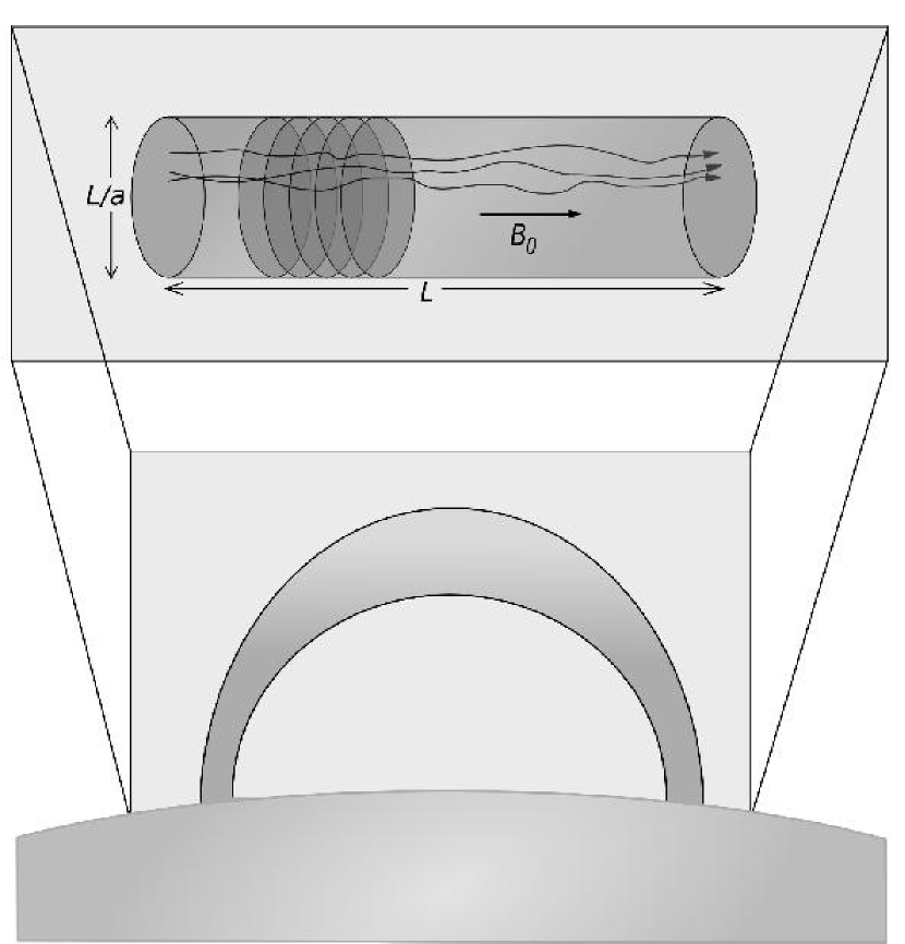
The “classical” GOY-like shell-model that we have just presented corresponds to MHD, where the average magnetic field has not yet been separated out; in the Shell-Atm model we present now in this paper, the average magnetic field is separated out, by starting from the RMHD equations (1-3). The new model we obtain corresponds basically to a pile of planes coupled by Alfvén waves and containing each a “classical” shell-model for 2D MHD (Fig. 1 top). This is similar to the loop model developed independently by Nigro et al. (2004), but the stratification of the atmosphere that we introduce allows to use this model in a large variety of cases of coronal loops or other structures (although we do not use this specific feature in the runs presented in this paper). In the Shell-Atm model:
-
•
The profile of the Alfvén speed along the mean field (i.e. the atmospheric structuring of the plasma) is given via a density stratification , an areal expansion factor of the flux tube and magnetic flux conservation. The latter two effects imply that the width of the loop and corresponding wavenumber must also, in general, depend on .
-
•
The Elsässer variables now depend on the position of the plane along the main axis of the simulation box, and the left hand-side of Eq. (5) is replaced by the term , corresponding to the linear Alfvén wave propagation in a stratified static atmosphere (Eq. 4). As a result, the external driving forces are not needed anymore, as energy can simply be input as an incoming energy flux at the boundaries.
-
•
The non-linear interactions occur inside each plane, in 2D. In this case the third invariant of MHD is anastrophy, i.e. the total square module of the magnetic potential ( with ). The coefficients of the non-linear terms of the shell-model are then those of Giuliani & Carbone (1998) with parameters and (i.e. and ).
To summarize, the fields of the Shell-Atm model we introduce and use in this paper are the complex variables , which are the Elsässer-like fields . is is the index of the shell, corresponding to the perpendicular wavenumber , with ; it can be any integer (positive or negative), but for numerical computations it is convenient to assume that is outside some domain 111The energy flux from the domain outwards is then zero, as can easily be seen using the equation of the spectral energy flux (14) for and .. is the position on the axis supporting , in a domain discretized over planes. The equations of the model are:
| (6) |
with given by Giuliani & Carbone 1998 (with , and ).
2.3. Quantities derived from the fields of the model
As represents the Elsässer field at perpendicular wavenumbers included in the shell and at position , is the energy per unit mass at position at time in the modes included in shell . If we assume that the modelled loop is a cylinder of diameter and that, after discretization in the direction, the separation between planes (i.e. the thickness of each plane) is , then the cross-section of the loop by a plane is and the volume associated to each plane is ; with a mass density , the mass associated to each plane is and the energy contained in the field is:
| (7) |
as a function of (for any field, position and time) will hereafter be referred to as the “shell energy spectrum”. To get a 1D perpendicular spectrum (as those given by turbulence theories), we need in addition to take into account the geometry of the shell in Fourier space: for a shell-model representing 2D MHD, has an area . It follows that the 2D energy spectral density in the shell is and that the 1D energy spectral density is . Note that for this reason there is a difference of between the slope of a power-law 1D perpendicular spectrum (e.g. for a spectrum as Kolmogorov, 1941) and the slope of its “shell energy spectrum” counterpart (e.g. ).
2.4. Scales of quantities of the model and time scales
The equations are rendered non-dimensional introducing characteristic units of time, length and density. For the coronal situation we choose for the unit of length, for the unit of time and for the unit of mass. Then the units of the other quantities derive naturally from these basic units and are for velocity, for mass density, for diffusivities, for energies, and for powers.
The characteristic time scales for each of the terms of Eq. (6) are deduced from their orders of magnitude:
| (8) |
where is an order of magnitude of the fields of the model at wavenumbers (parallel to ) and , and where represents either or . We obtain:
-
•
the Alfvén time ;
-
•
the characteristic time of dissipation ;
-
•
the characteristic time of non-linear interactions in the planes.
-
•
the wave reflection time scale .
The maximum Alfvén time is obtained for and corresponds to the time needed by the wave to cross the simulation box. By taking on the other hand the minimum of all the characteristic times in the box (using to get , to get , and ), we can estimate the time step needed by the numerical schemes according to Courant-Friedrichs-Lewy (CFL) conditions.
Other time scales also appear in the Shell-Atm model:
2.5. Case of a coronal loop
Geometry
For the case of coronal loops forced via photospheric motions, we consider the loops to be ”straightened out” as seen in Fig. 1 (bottom). This is similar to the cellular automaton model presented in Buchlin et al. (2003), but here the non-linear interactions between modes of MHD turbulence are represented through shell-models instead of cellular automata. Furthermore, for simplicity, we choose uniform density , Alfvén speed and loop width (); more realistic cases will be studied in future works.
Forcing
With this geometry, the boundary planes of the model represent the footpoints of the loop, which are anchored in the photosphere. We choose to impose a time-dependent vortex-like velocity field on modes at the larger scales, corresponding to photospheric convective motions at the scale of the supergranulation. Since the velocity is imposed, waves travelling along the loop are partially reflected at the photosphere.
The imposed velocity field on each mode of both boundary planes and has the form:
| (9) |
where is the amplitude of the forcing (non-zero only for some corresponding to scales of the supergranulation), and and are each independent random complex coefficients of module and whose complex argument is uniformly distributed over . These coefficients are kept constant during time intervals of duration , and they are randomly changed when and respectively, i.e. when the corresponding term is zero. This is another difference with the model of Nigro et al. (2004), who force using a stochastic velocity function on one boundary plane only. The auto-correlation time of the forcing field is then of the order of , which is chosen to be much longer than all the other time scales of the model (Sect. 2.4)
In practice, this boundary condition is realized by imposing an incoming Alfvén wave at the boundary and an incoming Alfvén wave at the boundary . The resulting power entering the loop is:
| (10) | |||||
Note that this power is not imposed, but it depends on the fields already contained in the simulation box.
3. Numerical simulations and analysis of the results
3.1. Energy
3.1.1 Energy balance
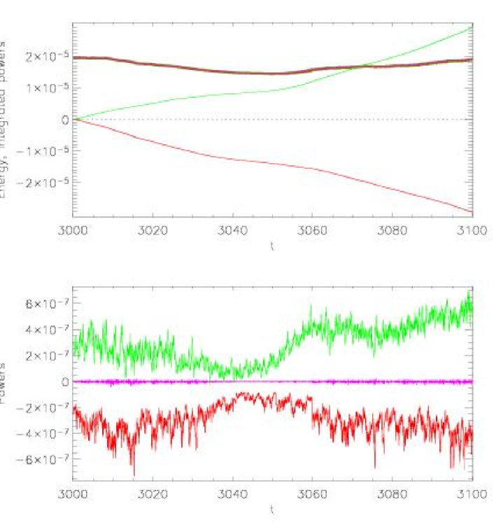
Alfvén wave propagation as well as the non-linear terms in our shell-model conserve the energy, so that changes in total energy in the loop arise only from flux through the photospheric boundaries (i.e. the forcing) and from the dissipation. This energy balance is well verified in practice, within in general as can be seen in Fig. 2, as long as the numerical dissipation due to the numerical scheme for wave propagation is not too high; the condition for this is that the perpendicular dissipation scales are not too small compared to the separation between planes in the direction.
3.1.2 Ratio of magnetic over kinetic energy
The ratio of the magnetic to kinetic energy in the stationary state may be estimated as follows. First, a simple linear estimate of the velocity field leads to:
| (11) |
while the magnetic field is given by:
| (12) |
The relative importance of the higher frequency modes to this low-frequency energy flux was discussed by Milano et al. (1997): given that the Alfvén wave travel times along loop is of the order of seconds, while most of the power in photospheric motions is in the minutes to hour ranges, it is the low-frequency resonance which plays a more important role. Energy injection from the photosphere into the corona therefore grows as , and is stored in the transverse coronal magnetic field, while the velocity field is bounded by its photospheric value. The linear solution will eventually break down because the magnetic field determined in Eq. (12) is not in general force-free and therefore will cause the coronal field to evolve dynamically. The ratio of magnetic to kinetic energies at this point may be estimated dimensionally by asking for the change in coronal velocity field determined by nonlinear interactions in Eq. (1) to be of the same order of magnitude as the field given by Eq. (11). Denoting the rms photospheric speed by , after a time the nonlinear term has the dimensional value , growing quadratically with time. It will cause a change in the coronal loop velocity field of the same order as over the time , when . One then recovers the time as where is the loop crossing time while is the non-linear time calculated on the photospheric velocity. The ratio of magnetic to kinetic energies in the corona at this stage is then
| (13) |
which we associate with the saturation level of magnetic to kinetic energies. This ratio should be a function of the aspect ratio of the loop. To check whether the Shell-Atm model follows this dependence, we perform a series of simulations with parameters , (i.e. a width ), , and for . The number of shells is and the number of planes is taken in the set with a separation between planes in all cases, leading to lengths and aspect ratios .
The ratio of magnetic energy to kinetic energy in the stationary state is plotted as a function of aspect ratio in Fig. 3, together with what is expected from Eq. (13). The numerical results we obtain support roughly this scaling, although the experimental ratios are smaller than the theoretical ratios by a factor and the values for an aspect ratio deviate from the scaling obtained for other aspect ratios. The slight departure from the proposed scaling, and the fact that the saturation level of magnetic to kinetic energy is lower than predicted, could be due to the ”leakage” of energy to the higher frequency resonances of the loop (as shown in Fig. 13).

3.2. Spectra
3.2.1 Formation of the spectra and spectral energy flux
The energy flux in each plane from the shells to the shells is the derivative of the energy contained in the shells due to the non-linear terms , namely:
| (14) | |||||
With we recover the hydrodynamic spectral energy flux given in Eq. (2) of Frick & Sokoloff (1998). Furthermore, this energy flux is consistent with the general idea that the energy flows “downhill” in the 1D perpendicular energy spectrum.
When starting the simulation from a very low amplitude field (Fig. 4), the magnetic energy and then the kinetic energy at the scales of the forcing grow, and when the fields are sufficiently large, non-linear effects become visible as energy is transferred to modes beyond those initially forced. In particular, there is a flux to higher mode numbers (, direct cascade), which continues to highest wavenumbers where dissipation occurs, as well as a flux to smaller wavenumbers (, inverse cascade) which energizes modes at the largest scales and saturates at a level comparable to the forced modes.

As a result of the energy cascade, an inertial range appears between the forcing and the dissipation scales, in the same way than in the original shell-models. The energy flux across shells is uniform on average over the whole inertial range. The Reynolds number in the case shown here can be evaluated to , which is much higher than any Reynolds number of direct numerical simulations. Even higher Reynolds numbers can be attained using more shells and planes, at the cost of the ability to do long-term statistics.
3.2.2 Fluctuations of the spectra
Once in the stationary phase, the spectra continue to fluctuate, with characteristic time scales linked to the “local” time scales, i.e. the time scales, as described in Sect. 2.4, considered as depending on the mode (Fig. 5). The most relevant time scale seems to be the local non-linear time scale , defined in 2.4, as this is the time scale on which the energy in a given mode can change under the action of the non-linear terms of Eq. (6). More precisely, no dynamics occur at time scales below the local non-linear time scales, as can be seen in Fig. 6: the modes with low have thus only long fluctuation times, excited by the long time scales of the forcing, while the modes with high fluctuate fast, but still with long characteristic times due to the flow of energy coming from the modes at low (these long-term fluctuations are common to the whole spectrum).

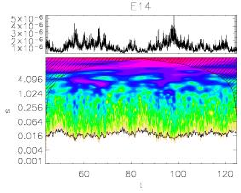
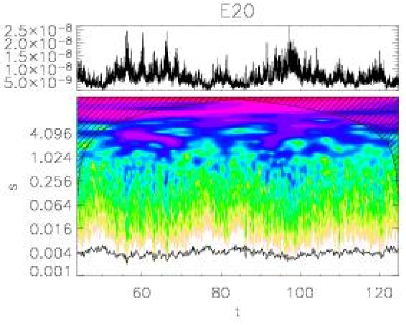

3.2.3 Evolution of the spectra during an event.
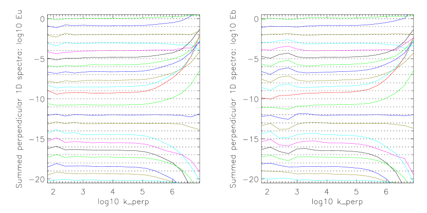
To understand what happens during episodes of high energy dissipation, we have analyzed the spectra of the fields before, during and after such an episode. The differences of spectra in respect to an average spectrum (Fig. 7) show that before the event (the maximum dissipation corresponds to the red spectrum differences), the energy accumulates over the whole spectrum. The total energy is then high, the non-linear times are short, and the energy flows down rapidly to the smallest scales according to Eq. (14): it enhances the spectra at the largest wavenumbers by several orders of magnitude, leading to a strong enhancement of the dissipation power. As energy is released, this process leads then to a decrease of the spectrum, first in the dissipative range (high wavenumbers), then in the whole spectrum. The dissipation power is then low again, and as the non-linear time scales in the inertial range are longer, the energy injected at the largest scales cannot flow to the smallest scales as fast as before: the energy does not reach easily the dissipative scales and the dissipation power remains low, until the next such episode.
Nigro et al. (2005) underline that the leading term of the energy flux across scales (Eq. 14) is proportionnal to (with the notations of the shell-model variables) and they also observe short-term variations of the kinetic energy spectrum around a dissipation event. These variations appear to control the energy flux to the smallest scales, and then the dissipation. In addition, we have shown that these variations exist on a longer term around an event, and that the magnetic energy spectrum also varies on the same time scales. The cross-scale energy flux may thus be controlled by both the kinetic and the magnetic energy spectra.

3.2.4 Slopes of the spectra
The slopes of the power-law 1D perpendicular spectra of the velocity and magnetic field (Fig. 4) seem to be roughly equal on the inertial range, but as the spectra fluctuate with time, there are fluctuations of the slopes. The distribution of these slopes obtained at different times is shown on Fig. 8: the median slope is (with a standard deviation ) for the velocity spectrum and (with a standard deviation ) for the magnetic spectrum. It appears that, on average, the kinetic spectrum is slightly steeper (by ) than the magnetic spectrum. If we look specifically at the times when the total dissipation power exceeds its 90th percentile, i.e. during events of energy dissipation, the spectra are slightly shallower, with medians of slopes being and for the velocity and magnetic spectrum respectively. This translates the fact that more energy is present at small scales during events of energy dissipation (red curves of Fig. 7).
These 1D spectra are different than the ones found by Nigro et al. (2005), corresponding to 1D spectra of slopes for velocity and for magnetic field; an explanation could be that their inertial range is smaller, and that their fitting range includes scales where forcing occurs.

3.2.5 Parallel and perpendicular spectra
In this model non-linear interactions occur only in perpendicular planes. Development of small scales along the magnetic field is then merely a consequence of the Alfvénic propagation of differences in the dynamics in different planes. One therefore expects parallel and perpendicular spectra to be different, with a relationship determined by the so-called critical balance condition, namely, that for a given perpendicular scale, differences in the parallel direction can appear only between planes such that the Alfvén propagation time is longer than the (perpendicular) non-linear time at that same scale (e.g. Goldreich & Sridhar, 1995; Cho et al., 2002; Oughton et al., 2004). In the case of the present model, assuming a 1D energy spectrum (i.e. a “shell energy spectrum”), the non-linear time scale is . With a constant and uniform advection velocity , the critical balance condition can be expressed by:
| (15) |
Note that with a Kolmogorov spectrum, we recover the result of Goldreich & Sridhar (1995).
For a field of the model at a given time ( can be , or ), let be its Fourier transform along the -axis. We obtain the two-dimensional power spectrum of (function of and ) from:
| (16) |
where is a constant.
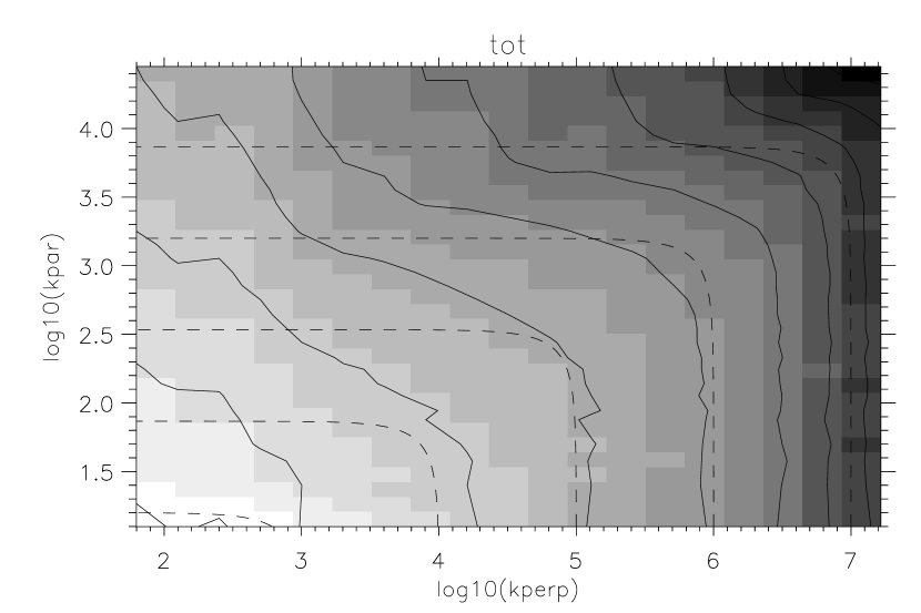
To get a sufficient wavenumber range in the parallel and perpendicular directions, we need to do simulations with a very large number of planes. This is achieved by starting a simulation with a number of planes , and then, once the energy has reached its final order of magnitude, by stopping the simulation and resuming it after having interpolated the fields in the direction. We can perform several steps of this process if needed. Figure 9 shows a 2D spectrum obtained by summing the and spectra and by averaging them over 10 times separated by , during a run with planes (runs with planes were also performed). The level lines in the space are clearly non-circular, and appear to follow the critical balance ellipses (Eq. 15) at large though with an excess of energy in the parallel direction. The anisotropy angle as defined by Eq. (5) of Del Zanna et al. (2001), computed on the range (where the spectrum is known as a function of both and ) is 67 degrees, which confirms that the spectrum is elongated in the perpendicular direction.
3.3. Dissipation, heating function and statistical properties
Heating function.
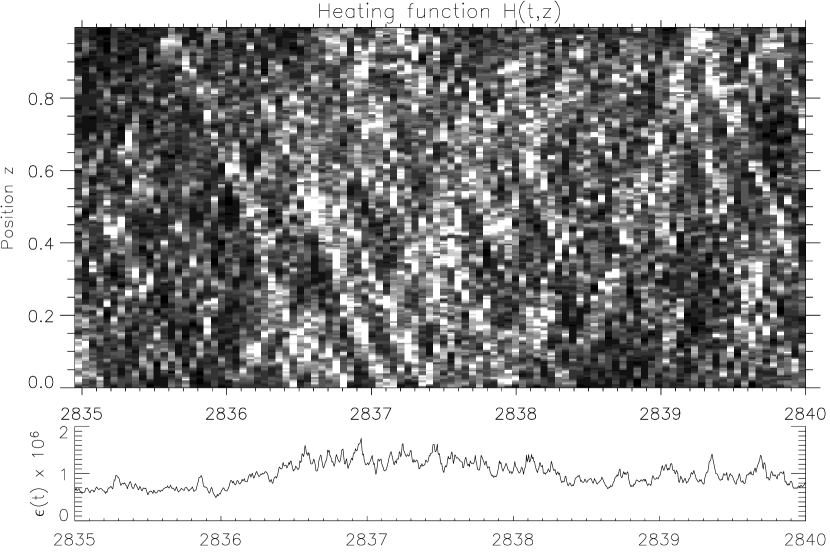
If we look at the energy dissipation power per unit length as a function of both time and position along the loop, we get the “heating function” (Fig. 10a). We see again (and for the same reasons than before) short-lived events of dissipations, and they correspond to short structures along the axis of the loop, whose size is of the order of the propagation distance of the structure during its lifetime. Some Alfvén wavepackets are also strong enough to be dissipated only after interacting with a lot of counter-propagating wavepackets, and thus they live a longer time and leave an oblique trace in the heating function during their propagation.
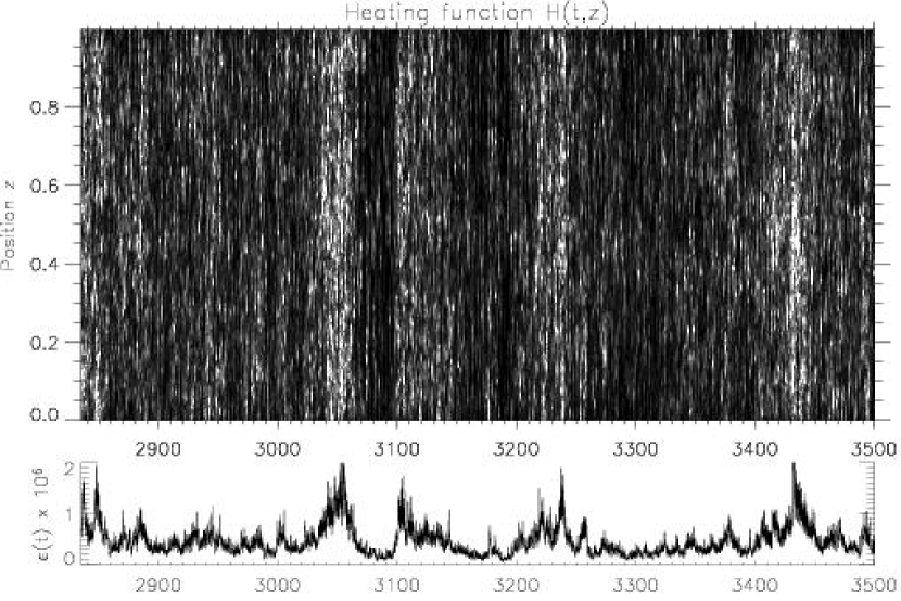
Furthermore, when we look at the heating function at long time scales of hundreds of crossing times (Fig. 10b), some features appear, which are related to the slow variations of the total energy (mainly contained in the slow-variating low- modes) under the effect of the slow forcing of time scale (which is chosen to be a few hundreds of ). The time variations of the dissipation power at these times scales (corresponding to a few minutes of physical time) seem to be almost the same on all positions along the loop. This is consistent with the common statement that the loop is heated as a whole, even though (1) the elementary events of dissipation, as seen in Fig. 10a, are each small compared to the length of the loop (2) thermodynamics, which would further smooth out the appearance of the heating function obtained from observable variables (because of the fast conduction times) has not yet been taken into account.
Dissipation power time series.
The integral of the heating function along the loop is the time series of the power of energy dissipation , shown in the bottom panels of Figs. 10(a-b). These time series display spikes of high dissipation power at short time scales during high-activity periods, as is usually found in both observations of solar flares and simulations of high-Reynolds number MHD turbulence. This dissipation time series will be analyzed further later.
Average profile of dissipation power.
On the other hand, the time average of the heating function, i.e. the average power of energy dissipation per unit length as a function of the position along the loop, shown in Fig. 10(c), is almost flat and drops only near the loop footpoints. This would suggest that coronal heating takes place almost uniformly along loops, although not at footpoints; however one must bear in mind that these simulations do not yet take into account realistic profiles of density and magnetic field.

Intermittency
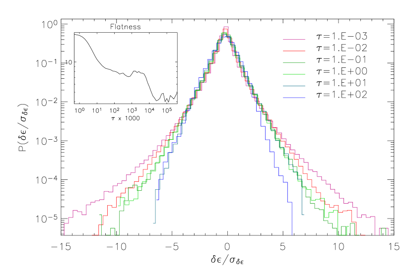
The increments of the time series at a given time lag have a distribution whose shape depends on the time lag : in Fig. 11, the distributions of the normalized by their standard deviation have wider wings for short time lags than for long time lags. Hence the time series is intermittent, which is confirmed by the rise of the flatness (fourth normalized structure function) for small time lags (inset of Fig. 11). This intermittency is a consequence of the intermittency that can be observed in the velocity and magnetic fields of the model, and which is also predicted by models such as She & Leveque (1994) in hydrodynamics and Politano & Pouquet (1995) in MHD. It could be a consequence of the fluctuations of the spectral flux resulting from the long-term global fluctuations of the spectrum which have been seen in Sect. 3.2.2. The modes with high are then intermittent, and as they participate the most to energy dissipation, the time series of energy dissipation power is intermittent.
Events
Statistics issued from observations often involve the detection of events, or structures, from the observed fields (Aschwanden et al., 2000; Parnell & Jupp, 2000; Buchlin et al., 2006), and the distributions of their characteristics. Following the “threshold” definition of Buchlin et al. (2005), with a threshold fixed at the average dissipation power, we get the distributions shown in Fig. 12 for the event total energy content, the peak power of energy dissipation, the duration of events, and the waiting-time between two successive events.
The distribution of the peak power in events is narrow, as a result of the summation of the heating function over the whole loop: the local spikes of energy dissipation are hidden by the average dissipation occurring in the whole loop. On the other hand the distributions of integrated dissipation power (total energy content of events) and of event durations are very wide. This is partially due to the threshold definition used (Buchlin et al., 2005), in the case of this time series where long time scales are superimposed to the shorter time scales of energy dissipation in the dissipation range. Furthermore, the waiting-times between successive events have also a wide power-law distribution. However, as discussed extensively in Buchlin et al. (2005), this result depends on what definition of an event is used to extract events from the time series of the power of energy dissipation.
Compared to the distributions of events obtained from the loop shell-model of Nigro et al. (2004), the main difference is the much steeper slope ( instead of ) of the distribution of the peak power in events. The reason could be the summation effect due to the existence of more but smaller dissipation events along the loop, because of the higher resolution we used in this run, both along the loop ( instead of , allowed by the parallelization of our code) and in the perpendicular direction ( instead of ).

3.4. Frequencies and time correlations
3.4.1 Frequencies
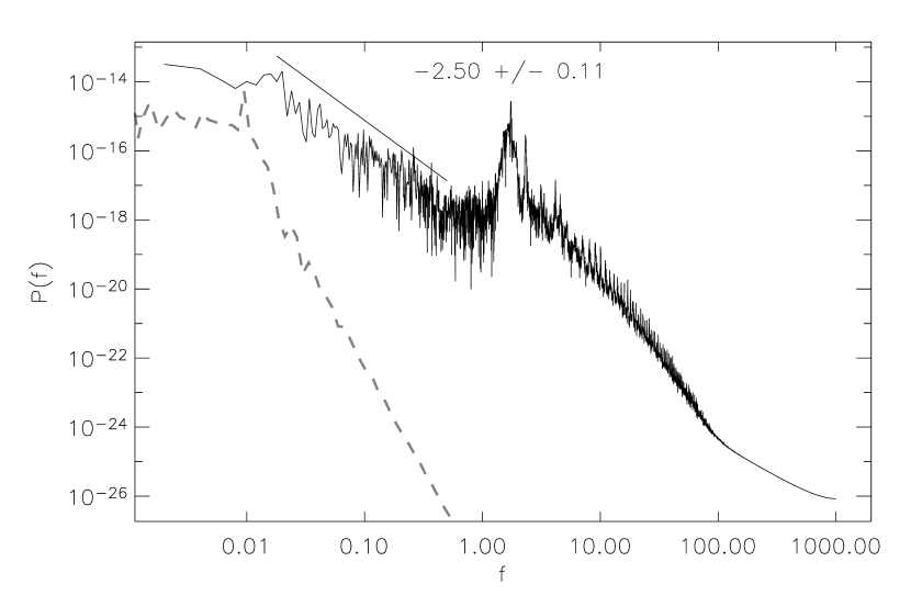
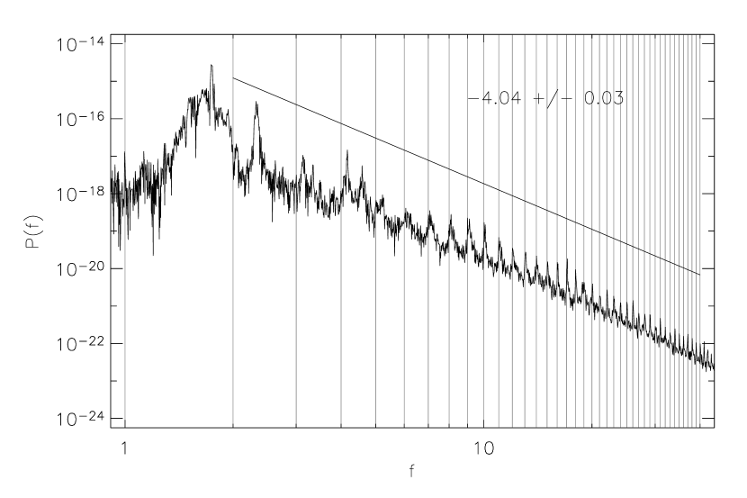
The time series of the kinetic and magnetic energies reveal oscillations corresponding to exchange of energy between the velocity and magnetic field. These exchanges occur, for example, thanks to the crossing of and wavepackets, and should have periods which vary depending on the precise number and repartition of wavepackets along the loop. A characteristic time scale is of course given by the Alfvén crossing time , corresponding to the first resonance frequency . Multiples of the Alfvén crossing time correspond to higher-frequency resonances of a loop in linear theory. While the power spectrum of the time series of total energy is a power-law of index over more than decades, the spectra of magnetic or kinetic energy display peaks corresponding to these resonances. The spectrum of the time series of kinetic energy (Fig. 13) fits to a power-law of index at very low frequencies. The first resonant frequency, together with the higher frequency harmonics, appear as peaks overlying a different, steeper power-law for the higher frequencies, shown in the bottom panel of Fig. 13. The frequencies of the peaks correspond well with the integer multiples of the fundamental for , while at lower frequencies they appear shifted. This shift, which is absent in a linear simulation (realized with the same parameters but without shell-models, i.e. with no non-linear interactions), is probably due to anharmonicity introduced by the non-linear effects, as shown by Milano et al. (1997) or Nigro (2005).
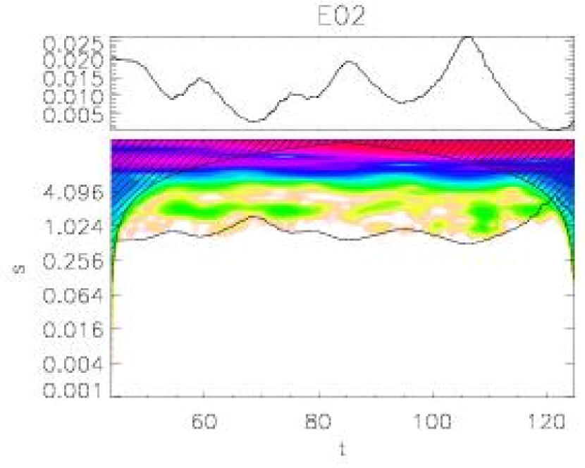
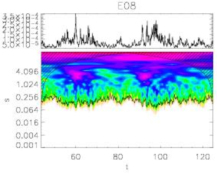
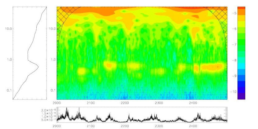
An even better understanding of these oscillations may be gleaned from a time-frequency analysis via wavelet transform shown in Fig. 14: there are oscillations which have long but finite lifetimes and different frequencies dominantly around the fundamental harmonic. These oscillating high-frequency wavepackets appear to arise in association with dissipation bursts, seen in the dissipation power time-series (bottom panel of Fig. 14). This intermittent rise in the high-frequency component of the velocity field may be involved in the enhanced non-linear interactions required to generate the bursts in power, as required in the flare-driving mechanism highlighted in Nigro et al. (2005). On the other hand, their persistence may be related to excitation by the time-space localization of the burst themselves, a sort of post-microflare resonant ringing, which might be observable with future high-cadence spectroscopic measurements.
The comparison between the spectra of the forcing function at a boundary and of the resulting energy time series (top panel of Fig. 13) makes it clear that the spectrum of energy is not contaminated by the spectrum of the forcing function, as the latter only contains very low frequencies, at or below ; this may not be the case with a stochastic forcing function as the one used by Nigro et al. (2004). This underlines the role of turbulence in providing the high frequencies which can resonate in the loop, viewed as a cavity for Alfvén waves, even in the absence of an external driver at these frequencies.
3.4.2 Auto-correlations
The correlation time of the energy time series is a few dozens of the loop crossing times by the Alfvén waves (Fig. 15), consistent with the slow evolution of the energy that we have already noted. The correlation time of the dissipation power time series is shorter, but still longer than the wave crossing time, as an effect of the weakness of the intermittent non-linear interactions between counter-propagation wavepackets and of the global long-term fluctuations of the spectrum (including the dissipation range) noted in Sect. 3.2.2.
3.4.3 Cross-correlations
A common goal when studying solar flares and space weather is to find precursors of flares, so as to get previsions of possible solar-terrestrial events (e.g. Abramenko et al., 2002; Abramenko, 2005; Georgoulis, 2005). With this heating model we can use the cross-correlations between time series to investigate which time series react first, and what kind of observations would be helpful when predicting flares. We have extended the study of Nigro et al. (2005), who show that in some events the kinetic energy begins to grow just before the start of a dissipation event, by doing a systematic correlation study between all energy and dissipation time series (kinetic, magnetic and total). Figure 15 shows the cross-correlations between the dissipation and the energy time series, as well as between the dissipation and the kinetic energy time series222Other correlations of pairs of time series of kinetic, magnetic or total energy or dissipations have not been plotted because they are very similar to either of the plotted correlations, as and .. Both cross-correlation functions show delays of the dissipations compared to the energy: the dissipation lags of approximately 5 time units compared to the total energy, and of approximately 0.5 time units compared to the kinetic energy (this last result is a confirmation of the result obtained in Nigro et al. 2005). Thus diagnostics methods based on the total energy or including the magnetic fields measurements may provide more useful results for space weather prediction than methods based on the velocity field alone. However, in both cases the delays involved are short, of the order of a minute at best.

3.5. Parametric study of dissipation power
Using the same runs as in Sect.3.1.2 (a set of loop with different aspect ratios for a fixed width), we compute the average energy dissipation in a stationary state, and we plot it versus the aspect ratio (Fig. 16): the scaling of the energy dissipation power per unit volume is approximately in . This scaling can be compared to the different models listed in Mandrini et al. (2000) and corresponds to heating of MHD in 2 dimensions.
As the slope of this power-law scaling is steeper than , shorter loops are more efficient in dissipation power per unit surface. This can be explained by the fact that Alfvén wavepackets that reflect on the loop footpoints interact more frequently in a short loop than in a long loop; as a matter of fact, simulations done when varying the Alfvén speed show that the average dissipation power also increases when the Alfvén speed increases. Assuming that the physical units of the model (see Sect.2.4 are , and , yielding , and , we get dissipation powers per unit surface between for large aspect ratios and for small aspect ratios. These values would be sufficient to heat the quiet corona (Withbroe & Noyes, 1977). Note however that they also depend on the physical properties and that we have assumed for the loop. Another series of runs has been performed to explore the influence of on the heating, and it gives ; this translates the fact that wavepackets interact more frequently when the Alfvén speed is higher, leading to more dissipation. These both fits, combined with a dimensional analysis on the variables (dissipation power per unit surface), (mass density), (Alfvén speed), (forcing speed) and (aspect ratio), give:
| (17) |
for the dissipation power per unit surface in S.I. units (), as a function of the other variables in S.I. units ( and ).

4. Conclusions
We have presented the Shell-Atm model, which is a generalization of shell-models (Giuliani & Carbone, 1998) with propagation of Alfvén waves along a field, with the further possibility of introducing a longitudinal stratification of physical properties (, mass density, flux tube expansion factor). Although the model is simple and includes only simplified physical processes, it has a very interesting complex non-linear dynamics and it is fast enough to get statistics of its fields and of the heating it produces: the simplifications we made allow to explore other properties than those accessible to classical direct numerical simulations (DNS). While it is not meant to replace and cannot replace DNS, for example because of the lack of three-dimensional information on field-line topologies, it partially fills the huge gap between the Reynolds numbers in DNS and in the real corona: although Reynolds numbers reached in the model, of the order of , are still lower than the ones expected in the corona, this already represents an outstanding progress compared to DNS. Furthermore this allows to explore regimes of MHD turbulence that are not accessible to DNS, for instance this allows for intermittency to appear in turbulence while having a complete description of the spectra and of the non-linear interactions in the perpendicular direction. On the other hand, having even higher Reynolds numbers, and thus smallest scales, may require to take into account non-MHD effects, like kinetic effects, that can still be neglected in this model.
The model has been used in this paper in the case of a magnetic loop in the solar corona, in which the physical properties of the medium (namely the external longitudinal magnetic field and the mass density) are assumed to be uniform along the loop. In this case, and thanks to the above-mentioned characteristics of the model, we could show that this model loop displays: a dynamics over a very wide range of spatial and temporal scales (4 to 5 orders of magnitude); spectra which are formed by a local cross-scale energy flux, and which have a wide inertial range in either direction, perpendicular or parallel to the external magnetic field; a clear anisotropy between the parallel and perpendicular spectra, which could be compatible with the “critical balance” phenomenology; a scaling of the average ratio of the magnetic energy over the kinetic energy consistent with RMHD; a heating function with multiple spatial and temporal scales; a flat longitudinal profile of the average dissipation power (although this may be dismissed by further simulations, with non-uniform physical properties of the medium along the loop); a spiky, and statistically intermittent time series of energy dissipation power; power-law distributions of the characteristics (peak energy, total energy, duration, waiting-times) of “events” extracted from the time series of dissipation power; finite-lifetime packets of resonant frequencies in the time series of energy, but whose frequencies are shifted from the harmonics of the linear resonant frequencies because of the non-linearities; long-range time correlations in time series; a delay of the dissipation time series compared to some energy time series; an average dissipation power that scales with the loop parameters, and that could be sufficient to sustain the high coronal temperatures. As discussed in the text, some of these results confirm or complete the results of a similar model (Nigro et al., 2004, 2005).
Further directions for the study of the solar corona using this model include taking advantage of the possibility of modelling non-uniform regions to (1) allow for density gradients in a coronal loop, to seek for the preferred locations of coronal heating, and (2) study a magnetically open region such as a coronal hole. In order to get diagnostics that can be compared to observations, this heating model can be coupled to the thermodynamics of a loop (including the cooling by conduction and radiation) upon which forward-modelling of coronal spectral lines may be carried out. We also believe that this model can be used in other heliospheric and astrophysical applications where MHD applies and where there is a strong dominant magnetic field (see Sect. A.3 in Appendix for code availability).
Appendix A The numerical code
A.1. Numerical schemes
The time advancement of the non-linear terms of the shell-models is performed by a third-order Runge-Kutta scheme. The Alfvén-wave propagation is done by the Fromm numerical scheme (Fromm, 1968). Finally, the dissipation terms of the shell-models can be computed by an implicit scheme. This allows to relax the CFL condition on and thus to fully resolve the dissipation range of the spectrum at no further computational cost.
A.2. Parallelization and parallel efficiency
The Shell-Atm model is parallelized using MPI, by simply distributing the planes over the processors. Communications are mainly needed for the propagation of the Alfvén waves between the domains corresponding to the different processors, and for the output. The resulting parallelization efficiency is good, and is even close to the ideal parallelization efficiency (up to hundreds of processors for ) thanks in particular to effects due to the cache size (when the number of processors grows, the local data get small enough to fit entirely in the level-2 memory cache of each processor).
A.3. Architecture of the code and availability
The Shell-Atm code is modular and can be adapted to a large variety of
physical systems. Different models for the non-linearities and different
numerical schemes can be chosen. We believe that the code can be useful for
the community and we have thus released it under the GNU GPL licence. The
code and its manual can be found at
http://www.arcetri.astro.it/ẽric/shell-atm/codedoc/.
References
- Abramenko (2005) Abramenko, V. I. 2005, ApJ, 629, 1141
- Abramenko et al. (2002) Abramenko, V. I., Yurchyshyn, V. B., Wang, H., Spirock, T. J., & Goode, P. R. 2002, ApJ, 577, 487
- Aschwanden et al. (2000) Aschwanden, M. J., Tarbell, T. D., Nightingale, R. W., et al. 2000, ApJ, 535, 1047
- Aulanier et al. (2005) Aulanier, G., Pariat, E., & Démoulin, P. 2005, Astron. Astrophys., 444, 961
- Biskamp (1994) Biskamp, D. 1994, Phys. Rev. E, 50, 2702
- Boffetta et al. (1999) Boffetta, G., Carbone, V., Giuliani, P., Veltri, P., & Vulpiani, A. 1999, Phys. Rev. Lett., 83, 4662
- Buchlin et al. (2003) Buchlin, E., Aletti, V., Galtier, S., et al. 2003, Astron. Astrophys., 406, 1061
- Buchlin et al. (2005) Buchlin, E., Galtier, S., & Velli, M. 2005, Astron. Astrophys., 436, 355
- Buchlin et al. (2006) Buchlin, E., Vial, J.-C., & Lemaire, P. 2006, Astron. Astrophys., 451, 1091
- Cho et al. (2002) Cho, J., Lazarian, A., & Vishniac, E. T. 2002, ApJ, 564, 291
- Del Zanna et al. (2001) Del Zanna, L., Velli, M., & Londrillo, P. 2001, Astron. Astrophys., 367, 705
- Desai et al. (1994) Desai, K. M., Gwinn, C. R., & Diamond, P. J. 1994, Nature, 372, 754
- Dmitruk et al. (1998) Dmitruk, P., Gómez, D. O., & DeLuca, E. E. 1998, ApJ, 505, 974
- Dmitruk et al. (2003) Dmitruk, P., Gómez, D. O., & Matthaeus, W. H. 2003, Phys. Plasmas, 10, 3584
- Frick & Sokoloff (1998) Frick, P. & Sokoloff, D. 1998, Phys. Rev. E, 57, 4155
- Fromm (1968) Fromm, J. E. 1968, J. Comp. Phys., 3, 176
- Georgoulis (2005) Georgoulis, M. K. 2005, Sol. Phys., 228, 5
- Georgoulis et al. (1998) Georgoulis, M. K., Velli, M., & Einaudi, G. 1998, ApJ, 497, 957
- Giuliani & Carbone (1998) Giuliani, P. & Carbone, V. 1998, Europhys. Lett., 43, 527
- Giuliani et al. (2002) Giuliani, P., Jensen, M. H., & Yakhot, V. 2002, Phys. Rev. E, 65, 036305
- Gloaguen et al. (1985) Gloaguen, C., Léorat, J., Pouquet, A., & Grappin, R. 1985, Physica D, 17, 154
- Goldreich & Sridhar (1995) Goldreich, P. & Sridhar, S. 1995, ApJ, 438, 763
- Gómez & Ferro Fontán (1992) Gómez, D. O. & Ferro Fontán, C. 1992, ApJ, 394, 662
- Heyvaerts & Priest (1992) Heyvaerts, J. & Priest, E. R. 1992, ApJ, 390, 297
- Isliker et al. (2000) Isliker, H., Anastasiadis, A., & Vlahos, L. 2000, Astron. Astrophys., 363, 1134
- Isliker et al. (2001) Isliker, H., Anastasiadis, A., & Vlahos, L. 2001, Astron. Astrophys., 377, 1068
- Kadomtsev & Pogutse (1974) Kadomtsev, B. B. & Pogutse, O. P. 1974, Sov. J. Plasma Phys., 1, 389
- Kinney & McWilliams (1998) Kinney, R. M. & McWilliams, J. C. 1998, Phys. Rev. E, 57, 7111
- Klein et al. (1991) Klein, L. W., Roberts, D. A., & Goldstein, M. L. 1991, J. Geophys. Res., 96, 3779
- Kolmogorov (1941) Kolmogorov, A. 1941, Dokl. Akad. Nauk. SSSR, 30, 299
- Lu & Hamilton (1991) Lu, E. T. & Hamilton, R. J. 1991, ApJ, 380, L89
- Lu et al. (1993) Lu, E. T., Hamilton, R. J., McTiernan, J. M., & Bromund, K. R. 1993, ApJ, 412, 841
- Müller et al. (2003) Müller, W., Biskamp, D., & Grappin, R. 2003, Phys. Rev. E, 67, 066302
- Mandrini et al. (2000) Mandrini, C. H., Démoulin, P., & Klimchuk, J. A. 2000, ApJ, 530, 999
- Milano et al. (1997) Milano, L. J., Gomez, D. O., & Martens, P. C. H. 1997, ApJ, 490, 442+
- Nigro et al. (2004) Nigro, G., Malara, F., Carbone, V., & Veltri, P. 2004, Phys. Rev. Lett., 92, 194501
- Nigro et al. (2005) Nigro, G., Malara, F., & Veltri, P. 2005, ApJ, 629, L133
- Nigro (2005) Nigro, G. 2005, PhD thesis, University of Calabria.
- Oughton et al. (2004) Oughton, S., Dmitruk, P., & Matthaeus, W. 2004, Phys. Plasmas, 11, 2214
- Oughton et al. (1994) Oughton, S., Priest, E., & Matthaeus, W. 1994, J. Fluid. Mech., 280, 95
- Parnell & Jupp (2000) Parnell, C. E. & Jupp, P. E. 2000, ApJ, 529, 554
- Passot & Sulem (2003) Passot, T. & Sulem, P. L. 2003, Phys. Plasmas, 10, 3914
- Politano & Pouquet (1995) Politano, H. & Pouquet, A. 1995, Phys. Rev. E, 52, 636
- She & Leveque (1994) She, Z. & Leveque, E. 1994, Phys. Rev. Lett., 72, 336
- Shebalin et al. (1983) Shebalin, J. V., Matthaeus, W. H., & Montgomery, D. 1983, J. Plasma Phys., 29, 525
- Strauss (1976) Strauss, H. R. 1976, Phys. Fluids, 19, 134
- Velli (1993) Velli, M. 1993, Astron. Astrophys., 270, 304
- Vlahos et al. (1995) Vlahos, L., Georgoulis, M., Kluiving, R., & Paschos, P. 1995, Astron. Astrophys., 299, 897+
- Withbroe & Noyes (1977) Withbroe, G. L. & Noyes, R. W. 1977, ARA&A, 15, 363
- Yamada & Ohkitani (1988) Yamada, M. & Ohkitani, K. 1988, Phys. Rev. Lett., 60, 983