Capella Corona Revisited: A Combined View from XMM-Newton RGS, Chandra HETGS, and LETGS
Abstract
We present a combined analysis of the X-ray emission of the Capella corona obtained with XMM-Newton RGS, Chandra HETGS, and LETGS. An improved atomic line database and a new differential emission measure (DEM) deconvolution method are developed for this purpose. Our new atomic database is based on the Astrophysical Plasma Emission Database and incorporates improved calculations of ionization equilibrium and line emissivities for L-shell ions of abundant elements using the Flexible Atomic Code. The new DEM deconvolution method uses a Markov Chain Monte-Carlo (MCMC) technique which differs from existing MCMC or -fitting based methods. We analyze the advantages and disadvantages of each individual instrument in determining the DEM and elemental abundances. We conclude that results from either RGS or HETGS data alone are not robust enough due to their failure to constrain DEM in some temperature region or the lack of significant continuum emission in the wavelength band of the spectrometers, and that the combination of HETGS and RGS gives more stringent constraints on the DEM and abundance determinations. Using the LETGS data, we show that the recently discovered inconsistencies between the EUV and X-ray lines of Fe XVIII and XIX also exist in more highly charged iron ions, up to Fe XXIII, and that enhanced interstellar absorption due to partially ionized plasma along the Capella line of sight may explain some, but not all, of these discrepancies.
1 Introduction
The Capella system is one of the strongest X-ray emitting coronal sources, and has been observed numerous times with the past and current X-ray observatories, including both High and Low Energy Transmission Grating Spectrometers (HETGS, LETGS) on board Chandra and the Reflection Grating Spectrometer (RGS) of XMM-Newton. Capella is a close spectroscopic binary with an orbital period of 104 days and a distance of 12.9 pc (Hummel et al., 1994).
The general features of the temperature distribution of the Capella coronal plasma were reasonably well determined, even with the previous generation X-ray and EUV observatories, equipped with limited spectral resolutions. Observations with the EUVE spacecraft have shown a continuous differential emission measure (DEM) distribution over a temperature range of to K (Dupree et al., 1993). Brickhouse et al. (2000) analyzed the simultaneous observations of EUVE and ASCA, and concluded that the DEM is sharply peaked near K. The abundances of Mg, Si, S, and Fe were found to be consistent with solar photospheric values, and Ne was found to be underabundant by a factor of to 4 in that analysis.
Since the launch of Chandra and XMM-Newton, high resolution X-ray spectra have become available, and numerous analyses of the Capella coronal X-ray emission have appeared using all three grating instruments. The first light observations were presented by Canizares et al. (2000) for HETGS, Brinkman et al. (2000) for LETGS, and Audard et al. (2001) for RGS, which gave an overview of the spectral data using relatively simple analysis methods. Behar et al. (2001) investigated in detail the Fe L-shell line emission using the HETGS data and theoretical calculations of the Hebrew University Lawrence Livermore Atomic Code (HULLAC). Phillips et al. (2001) made detailed comparisons between the HETGS X-ray spectra and extreme-ultraviolet emission from EUVE. Mewe et al. (2001) presented temperature, density and abundance diagnostics using the LETGS observation and a line ratio based analysis method. Argiroffi et al. (2003) studied the structure and variability of the X-ray corona using multiple LETGS observations and a Markov Chain Monte-Carlo (MCMC) method for the DEM deconvolution developed by Kashyap & Drake (1998). The x-ray emission are found to be constant to within a few percent on both short and long time scales. Audard et al. (2003) studied the coronal abundances and the first ionization potential (FIP) effects of several RS CVn binaries, including Capella, using the XMM-Newton observations.
All previously mentioned analyses have relied on a single grating instrument in the X-ray band. Desai et al. (2005) combined multiple HETGS and LETGS observations and investigated various line ratios of Fe XVIII and XIX. Large discrepancies of a factor of two were found between the observed and theoretical ratios involving X-ray transitions and EUV resonance lines. It was assumed that such discrepancies reflect the uncertainties of theoretical atomic data. However, this combined analysis was not aimed at deriving coronal properties of Capella.
Because of the different spectral coverage of the three grating instruments, it is conceivable that a joint analysis of all instruments may yield more stringent constraints on the DEM distribution and elemental abundances of the capella corona than that of individual instruments. Although observations with three gratings are generally not simultaneous, a joint analysis is possible due to the lack of variability of X-ray emission as indicated by multiple observations with individual instruments. In this paper, we present such a combined analysis of observations with HETGS (ObsID 5040, 28 ks), LETGS (ObsID 1248, 84 ks), and RGS (ObsID 0121920101, 51 ks). Many more similar observations exist for all instruments. The three are chosen more or less randomly. The primary goal of the present work is to introduce our analysis method and discuss the complementary nature of the three instruments. The statistical quality of these individual observations are sufficient for this purpose. We leave a systematic investigation of all available data for future work.
In the course of this work, we have developed an improved atomic line database and a new DEM deconvolution method. The new atomic line database is based on the line list of astrophysical plasma emission code (APEC) of Smith et al. (2001) with the L-shell emission lines from Ne, Mg, Al, Si, S, Ar, Ca, Fe, and Ni replaced with calculations using the Flexible Atomic Code (FAC) developed by Gu (2003a). Our new MCMC DEM deconvolution method is an adaptation of the spatial-spectral analysis procedure of Peterson et al. (2006) to the analysis of pure spectral data, and is different from the MCMC method of Kashyap & Drake (1998) in technical details.
In §2, we describe our improvements to the atomic line database of APEC; in §3, the details of the MCMC method for DEM deconvolution are discussed; §4 and §5 present the analysis of the XMM-Newton RGS and Chandra HETGS observations respectively; §6 presents the joint analysis of RGS and HETGS data; In §7, the additional constraints on the physical properties of the interstellar medium along the Capella sight line imposed by LETGS data are analyzed; we conclude with brief discussions of the results in §8.
2 An Improved Atomic Line Database
A complete and accurate atomic database is the cornerstone of X-ray spectroscopy. The high resolving power of Chandra and XMM-Newton grating spectrometers have made it even more important because many previously unresolved line transitions become well isolated in the new observations. There has been a concerted effort, both experimental and theoretical, to improve the existing atomic data in the past decade. For example, the widely used MEKAL plasma model has gone over major revisions in its implementation in the SPEX package. Smith et al. (2001) have developed a new plasma emission code and its associated atomic data, combining the most recent theoretical and experimental results for many important transitions, particularly those from iron L-shell ions. This database and the code, astrophysical plasma emission database and code (APED/APEC) are routinely used in the analyses of Chandra and XMM-Newton grating data.
Despite the numerous improvements and greatly enriched line list in APED/APEC over its predecessors, there are some deficiencies in its most recent version. Firstly, the collisional ionization balance used in the code are based on the recombination and ionization rates compiled by Mazzotta et al. (1998). Gu (2003b) showed that there are some systematic problems with dielectronic recombination (DR) rate coefficients used there for some L-shell ions of astrophysically abundant elements, including iron. The ionization fractions calculated using the new DR rate coefficients of Gu (2003b) can be different from that of Mazzotta et al. (1998) by as much as a factor of two for some ions. Secondly, the line emissivities of L-shell ions in APED/APEC are mostly based on the distorted-wave calculations of HULLAC, and do not take into account the roles of resonances. Gu (2003a) and Doron & Behar (2002) demonstrated that not only do resonances play an important role in forming X-ray lines for L-shell iron ions, but also the DR of next higher charge state contributes to the line emissivities. Thirdly, the transition wavelengths of L-shell ions have primarily relied on HULLAC calculations except for a subset of lines from the iron ions where experimental measurements of Brown et al. (1998) and Brown et al. (2002) are used. HULLAC wavelengths are known to have limited accuracy insufficient for the analysis of Chandra and XMM-Newton grating spectra. Lastly, the L-shell line models for less abundant elements such as Si, S, Ar, and Ca are not as sophisticated as that for Fe, and do not contain as many transitions.
We have modified the APED/APEC line list by replacing all L-shell emission lines of Ne, Mg, Al, Si, S, Ar, Ca, Fe, and Ni with our own calculations using the atomic data produced by the Flexible Atomic Code. For the lines of Fe ions, we use the data of Gu (2003a), which includes resonance excitation, recombination and ionization processes as population mechanisms. For other lines of Fe and other elements, we have calculated direct excitation only models including levels up to . The ionization fractions of all L-shell ions are calculated with the DR rate coefficients of Gu (2003b) in our new models. We have used the many-body perturbation calculation of Gu (2005) for the wavelengths of lines of Fe and Ni ions, which have been checked against the measurements of Brown et al. (1998) and Brown et al. (2002) for strong Fe lines and deemed accurate to within a few mÅ. For the L-shell lines of S, and Ar, we have replaced the theoretical wavelengths with experimental ones for those identified in the measurements of Lepson et al. (2003) and Lepson et al. (2005). We calculated our emissivities in the low density limit, which is appropriate for the majority of lines at stellar coronal densities in general, and for Capella in particular. Some lines in the lower Z ions may have been affected by density effects. We estimate that such effects are not severe at the relatively low density of the Capella corona, and do not attempt to correct for them.
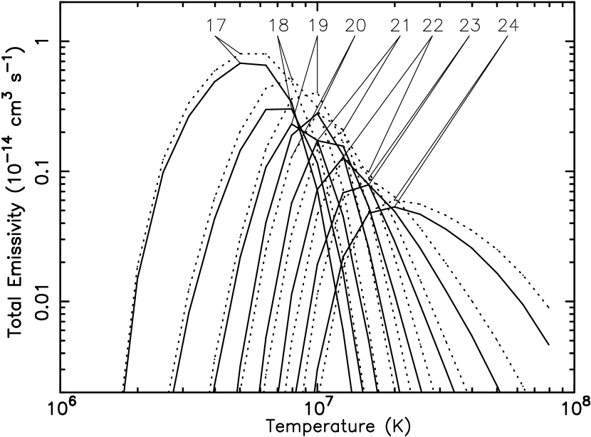
The result of our modification to the APED/APEC line list is a vastly enlarged line model with more accurate wavelengths and emissivities for L-shell ions. The new line list is stored in the same FITS format as the original one, and can be used in any analysis software that already incorporates APED/APEC plasma models. To illustrate the main differences between our new line list and the original APED/APEC list, we show the comparison of total emissivities of Fe L-shell ions in the 5–20 Å spectral region as functions of temperature in Figure 1. The emissivities in our new database are generally larger than those of APED/APEC, reflecting the inclusion of resonances and recombination contributions to the level population and the modification to ionization equilibrium fractions. Enhancements of more than a factor of two are seen at certain temperature ranges for some ions. For Fe XVIII and XIX, even the differences in peak emissivities reach a factor of 1.7. In Figure 2, we show the total emissivities of L-shell ions of Si, S, Ar, Ca, and Ni in the 5–40 Å spectral region as functions of temperature. It is seen that our new emissivities are also generally larger than the original APED/APEC database. The differences in the Ni emissivities are relatively small, while for other elements, they can be quite larger at temperatures of 1–5 K. We also note that our new data does not exhibit the irregular temperature variation for Ar and Ca emissivities, as does the APED/APEC. In the next section, we will examine the differences between the two line models in further detail when they are applied to analyze some simulated data using our DEM deconvolution method.
3 A New Differential Emission Measure Deconvolution Method
Differential emission measure (DEM) distribution is one of the fundamental properties of stellar coronae. It characterizes the temperature structure of the coronal plasma, and is the main objective of X-ray spectroscopic analyses. Many techniques have been developed to derive DEM from X-ray or EUV spectroscopic data. For low resolution instruments such as the solid state detectors of ASCA, simple multi-temperature model fitting methods are usually favored since individual emission lines cannot be resolved. For high resolution instruments, the first step in deriving DEM in almost all existing methods is to identify individual lines from different ions and measure their fluxes. In the simplest method, one then assumes that each ion emits at the temperature of peak emissivity. The amount of emission measure at that temperature is then derived by dividing the flux by the peak emissivity, assuming known abundance of the emitting element. The discrepancy between the emission measure derived with different elements but at similar temperatures can be used to infer the deviation of the elemental abundances from the assumed values. In more advanced techniques, one may try to infer the DEM and elemental abundances simultaneously by matching the model and measured line fluxes and continuum level. The actual matching procedure may take the form as fitting or MCMC simulations.
Using the measured line flux as the starting point has its advantages and disadvantages. The main advantage is that accurate theoretical wavelengths of transitions and wavelength calibration of the instruments are not critical as long as lines can be reliably identified, while the disadvantage is that it requires the lines to be well resolved to be useful in this procedure. However, even with the high resolution of Chandra and XMM-Newton grating spectrometers, many lines still blend with each other and their fluxes are difficult to measure individually. With the wavelengths of all major strong lines known to a high accuracy either through laboratory measurements or many-body perturbation calculations, we find that a global fitting method to the raw spectrum is feasible and is our preferred method because it takes into account all lines and continuum emission on equal footing. The possible effects of wavelength uncertainties in the database will be discussed in more detail later in this section. In our analysis, we also work with the raw spectra without rebinning. The problem of low photon counts are taken care of by using the Poisson likelyhood throughout the entire spectral region.
One still needs to decide how the DEM is to be parameterized and the actual fitting technique to be used. Clearly, the parameterization of the DEM and the abundances of major cosmic elements requires a fairly large parameter space. The traditional minimization methods are not only inefficient but often easily trapped in local minima. The MCMC method is a natural choice for such problems. In addition to using a global fitting method instead of line flux based techniques, we also choose a different parameterization framework from the MCMC method of Kashyap & Drake (1998). In the method of Kashyap & Drake (1998), the DEM distribution is discretized on a suitable temperature grid, and the emission measure value at each temperature bin is treated as a parameter. Our method is an adaptation of the more sophisticated technique of smoothed particles inference for spatial-spectral analysis (Peterson et al., 2006) to the pure spectral data. In this method, the plasma is represented as a set of smoothed particles with identical emission measures at different temperatures. In the spatial-spectral analysis, each particle has a Gaussian shape in spatial extension. In the pure spectral case as applicable to the stellar coronae, we ignore the spatial extension, and each particle becomes a basic luminosity block at certain temperature. In other words, the DEM is represented by a multi-temperature model
| (1) |
where the emission measure normalization at each temperature, , is the same, and given by the global parameter . Unlike the parameterization of discretizing the DEM over a fixed temperature grid, here the temperatures of luminosity particles are taken as free parameters. The peaks and valleys in the DEM therefore correspond to greater or lesser concentrations of these particles in certain temperature regions. Initially, the temperatures of the particles are drawn randomly from a uniform distribution on the logarithmic scale over a suitable temperature range. They are then iterated in the MCMC process along with all other required parameters for the plasma, such as the interstellar absorption and elemental abundances. When the Markov Chain has reached equilibrium, the histogram of the set of temperatures in each iteration provides an estimate of the DEM distribution. The average of this histogram along the equilibrium chain gives the smoothed DEM with greatly reduced statistical noise, and is taken as the final result. The variance of the histogram is taken as the statistical uncertainty of the emission measure in each temperature bin. Other plasma parameters and their uncertainties are similarly estimated by taking averages and variances along the Markov chain. We implemented our method as a custom-built fit method in the Interactive Spectral Interpretation System (ISIS, Manset et al. (2000)), and the analysis presented below are all carried out using ISIS.
The main advantage of this parameterization procedure is that the DEM distribution is naturally and adaptively smoothed over a temperature scale comparable to the width of emissivity profiles of individual lines. Such smoothing is realized by the random walk of the temperature particles and the averaging of temperature histograms over a long Markov chain in equilibrium. If one parameterizes the DEM over a fixed temperature grid, some regularization technique must be employed to ensure the smoothness of the distribution, and such smoothing must be predetermined regardless of how much is actually required by the data and model. Even though our new parameterization requires a large number of parameters as we typically use 100-200 temperature particles to represent the DEM distribution, it is found to perform quite robustly in our tests. In particular, it always finds the DEM solution consistent with the data and without overly sharp features, as we demonstrate below.
Another advantage of our parametrization is the relatively small correlations between all parameters, except for the overall normalization parameter, , and the overall absolute abundance, which are the only two that are highly correlated. In order to avoid dealing with this high correlation, we stop iterating the parameter after a certain number of iterations when the MCMC chain has entered the equilibrium state, and a reasonable estimate of has been found. This way, we only adequately sample the parameter space that defines the shape of the DEM and the relative abundances. Therefore the statistical uncertainties of abundances given by our analysis are only meaningful in a relative sense.
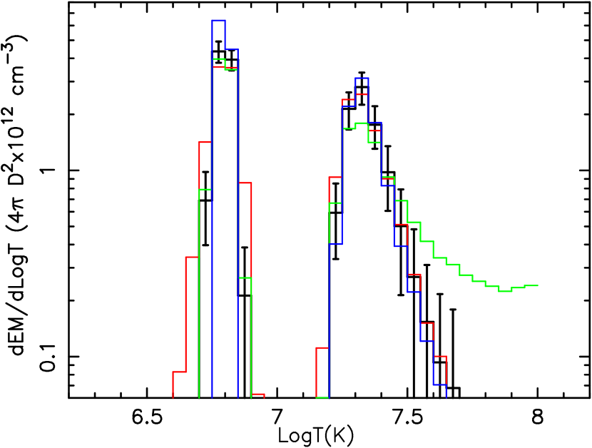
In our first test, we simulate a two-temperature thermal plasma with and . The total emission measure in the two components are equal and is cm-3, where is the distance of the source in cm. We assume solar abundances and no interstellar absorption in the model. The spectrum is then folded through instrument responses to generate fake data for 60 ks observations for both HETGS and RGS, which are analyzed by the present MCMC method. The total emisssion measure and exposure time chosen here make the spectra in both HETGS and RGS comparable to the Capella data analyzed in this work. During the analysis, we use 100 temperature particles. The abundances of all heavy elements are tied as a single parameter but are allowed to vary. Including the overall normalization factor, , a total of 102 parameters are therefore required to characterize the plasma model. The MCMC chain is 2000 iterations long, and we exclude the first 500 iterations as the burn-in period. Through visual inspection of key parameters, we determine that 500 burn-in iterations are more than enough to allow the MCMC chain to enter the equilibrium state. The test is designed to illustrate how the method behaves when the underlying DEM has two sharp peaks. The MCMC analysis is performed three times, on MEG data alone, on RGS data alone, and jointly on MEG and RGS data. The three versions of the reconstructed DEM are shown in Figure 3 with red, green and black histograms. It can be seen that the two temperature peaks are resolved in our reconstructions, but each has a finite width. This is because the line emissivity profiles that constrain the DEM at the relevant temperatures have finite widths and it is simply not possible for any method to resolve structures sharper than these emissivity profiles allow. We also note that the high temperature peak is broader than the low temperature one. This is because the lines that constrain the high temperature DEM are mainly from K-shell ions, and have broader emissivity profiles. The high temperature peak reconstructed from RGS data is broader than those from MEG or the combination of MEG and RGS, reflecting the short wavelength cutoff of the RGS effective area. The derived abundance is from MEG, from RGS, and from the combination of MEG and RGS. The uncertainties are quoted at 90% confidence level, and are calculated from the variance of the MCMC chain. These abundance values range from 10–30% larger than the solar value used in the generation of the simulated data. However, this overestimation of abundance is offset by the corresponding underestimation of total emission measure in the reconstructed DEMs, and therefore the product of emission measure and the abundance agrees with the input model very well. This mismatch is due to the fact that for this test case, there is only a weak continuum in both MEG and RGS wavelength bands. It is the ratio of line to continuum emission that constrains the abundance value. With weak continuum, it is difficult to reproduce the total emission measure and abundance independently, even though the shape of the DEM and the product of the total emission measure and the abundance can be reliably determined. The uncertainties associated with this difficulty are not represented in our analysis, because we stop iterating the overall normalization parameter, , when a reasonable estimate has been found. To verify that the deviations in the derived absolute abundance values are in fact consistent with the statistical properties of the data, we evaluate the maximum likelyhood statistics as an indication of the goodness of fit. This statistics is defined as
| (2) |
where is the Poisson likelyhood. This definition ensures that approches the conventional value when all bins have sufficient counts to be approximated by normal distributions. Take the reconstruction from MEG as an example, the value for the final model is 23651 in the 3 to 27 Å range of both orders of spectra, with 9600 total number of bins. If we fix the abundance at the solar value and repeat the MCMC analysis, the final value is 23618, i.e., 33 smaller than the case with a varying abundance. However, the variance of for random data are expected to be , where . In fact, by generating many copies of the random data, we verify that is well approximated by a normal distribution with standard deviation of , and mean of 23297. In other words, our reconstruction with overestimated abundance and underestimated total emission measure does not differ statistically from the model with the correct abundance, although both deviate from the “perfect” model by about 2.5.
To illustrate the effects of differences between our new atomic line database and the original APED/APEC list, we carry out a further analysis. We take the joint MEG and RGS data generated using the new atomic line list, and analyze them with the original APED/APEC database. The reconstructed DEM is also shown in Figure 3 as the blue histogram, and the corresponding abundance is 1.15. Clearly, for this test case, the results are not very different from the one obtained with the “correct” atomic line list, except that the low temperature peak appears to be much narrower now. However, the value of the fit is larger than that of the “correct” model by 3070, which is much larger than the expected statistical deviation.
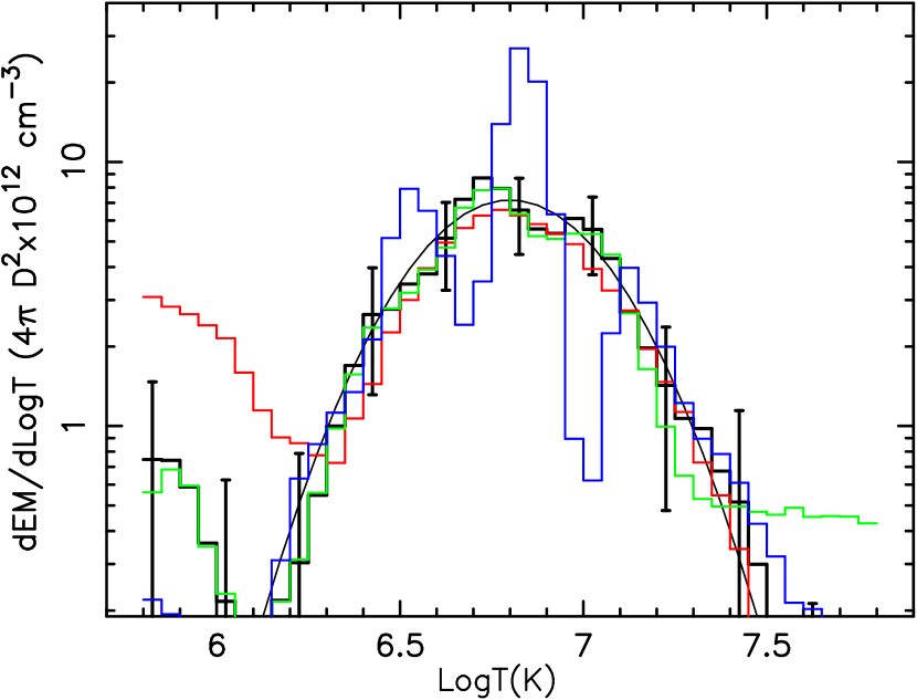
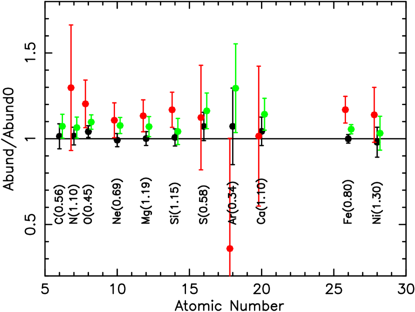
In our second test, we simulate a thermal plasma with a broad DEM distribution. The distribution has a Gaussian profile in , which is centered at 6.8 and has a standard deviation of 0.25. This DEM somewhat resembles the main peak in the DEM reconstructed from the Capella data in §6. The total emission measure is cm-3, which is also comparable to the Capella corona. Fake MEG and RGS spectra are generated with exposure times identical to the actual Capella observations used in the present work. Therefore the statistical quality of the simulated spectra are similar to the Capella data analyzed in this work. We also adopt the elemental abundances derived from the Capella data, and allow all abundances to be free parameters in the reconstruction. Like in the first test case, the MCMC analysis is performed three times, on MEG data alone, on RGS data alone, and jointly on MEG and RGS data. The three versions of the reconstructed DEM are shown in Figure 4, and the derived abundances are shown in Figure 5. It is seen that the three reconstructions are generally consistent with each other, and with the input Gaussian distribution. MEG data does not constrain the DEM below , and the RGS data produces excessive emission measure above . As in the first test case, due to the lack of significant continuum emission, both MEG and RGS data give a total emission measure slightly smaller than the input model, while the abundances are slightly above the input values. MEG data also gives larger uncertainties to the derived abundances, with several elements practically unconstrained. The joint fit of MEG and RGS data gives best constrained abundance values, which are consistent with the input model.
The effects of using the original APED/APEC line list to analyze the spectra simulated with our new atomic data are also investigated for this test case. The blue histogram in Figure 4 shows the resulting DEM reconstruction from the combination of MEG and RGS data. In this case, we notice that the reconstructed DEM gives sharper structures and suggests multiple peaks. The deviation from the “correct” model is much larger in this case than in the first test. We believe that it is due to the irregular temperature variations of emissivities for some Fe L-shell ions. When the original APED/APEC line list is used to analyze real astrophysical spectra, we also notice that it always generates more peaks than if we use our new atomic line database. Since the fits using our new line list always provide significantly higher qualities, we conclude that our new database is more realistic than the old one.
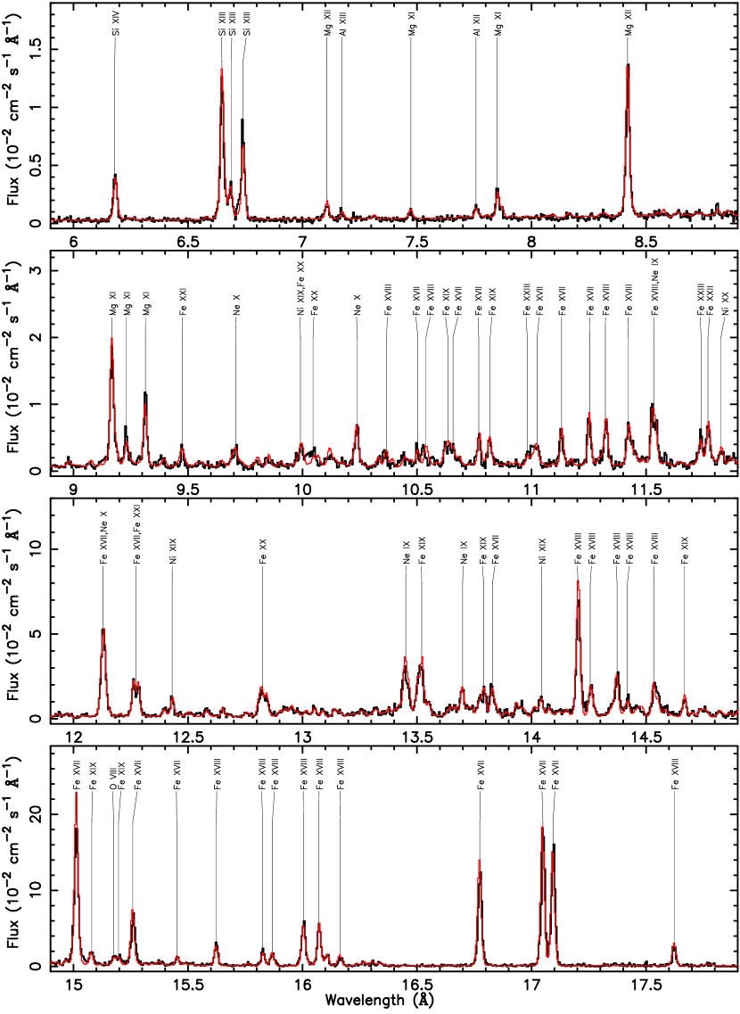
Another major concern in a global fit method such as the one used here is whether uncertainties in wavelengths may bias the results. In our new database, the wavelengths of lines of L-shell ions of Fe and Ni are obtained with a many-body perturbation calculation (Gu, 2005), whose accuracy has been verified by comparison to the laboratory measurements of Brown et al. (1998) and Brown et al. (2002). We are confident that wavelengths errors for these lines are on the order of 5 mÅ or less. For the strongest transitions of S and Ar L-shell ions, the wavelength measurements of Lepson et al. (2003) and Lepson et al. (2005) are used. The wavelengths of high- transitions of Fe ions may have slightly larger uncertainties in our database. However, these lines are generally weaker and provide less constraints in the DEM reconstruction. The overall good quality of fit shown in Figure 10 corroborates our error estimation. To investigate the effects of such small wavelength uncertainties on the results, we constructed an atomic line list by perturbing the wavelengths with Gaussian random errors of 5 mÅ standard deviation, and used that to analyze the simulated data. In both test cases discussed above, the resulting reconstructions are the same as the ones obtained with unperturbed wavelengths to within a few percent for both DEMs and abundances.
These two tests illustrate that when the underlying DEM has sharp features, our method generates a smoothed reconstruction consistent with the line emissivity profiles, and when the DEM is a continuous distribution, our reconstruction agrees with the true DEM very well when the MEG and RGS data are used jointly. However, such good reconstruction quality depends on the assumption that one has the perfect knowledge of atomic database and instrument calibration. In the analysis of real astrophysical spectra, the unknown uncertainties in these factors may lead to systematic errors in the reconstruction.
4 XMM-Newton RGS Data
We first apply the above method to the XMM-Newton RGS data. As in the test cases, a total of 100 temperature particles are used in the MCMC analysis. The temperatures are restricted in the and K range. Initially, the temperatures are distributed uniformly on the logarithmic scale. The abundances of C, N, O, Ne, Mg, Si, S, Ar, Ca, Fe, and Ni are allowed to vary in the fitting, and the interstellar absorption is fixed at the value determined by Linsky et al. (1993), which is cm-2. The elemental abundances in our analysis are measured in units of solar photospheric values (Anders & Grevesse, 1989). RGS1 and RGS2 spectra are jointly fit. Including the overall normalization factor, a total of 112 parameters are needed to characterize the plasma model.
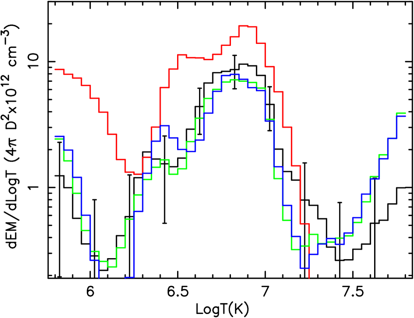
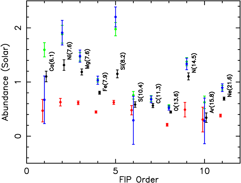
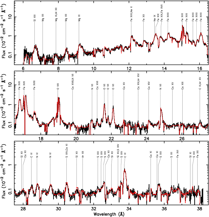
Because Capella is a bright source and XMM-Newton RGS has decent effective area at long wavelengths, numerous L-shell lines of intermediate-Z elements, such as Si, S, Ar, and Ca are clearly detected. The L-shell ions of these elements are present at relatively low temperatures, while their K-shell counterparts are generated in higher temperature regions. Assuming that the same elements in different regions have the same abundances, the presence of both L-shell and K-shell lines in the spectrum provides important constraints on the emission measure of low and high temperature regions. Without these L-shell lines, the lower temperature DEM is primarily constrained by K-shell lines of low-Z elements, while higher temperature DEM is constrained by L-shell lines of Fe. It would therefore be more difficult to determine the ratio of low and high temperature DEMs without knowing the abundance ratios of low-Z elements and Fe. Moreover, for some elements, such as S, Ar, and Ca, the K-shell lines are not detected by RGS, and their abundances are only constrained by the L-shell lines. To illustrate the effects of these L-shell lines, we carried out two fits. One includes the entire spectral region from 6 to 38 Å, and the other excludes some regions where strong L-shell lines of Si, S, Ar, and Ca are identified, primarily above Å. The resulting DEM reconstructions are shown as the green and blue lines in Figure 6, respectively. The abundance measurements are shown as green and blue symbols in Figure 7. The summed RGS1 and RGS2 spectrum and the best-fit model are shown in Figure 9. The reconstructed DEMs are dominated by a broad peak near and a smaller secondary peak near . It is seen that the main differences between the two DEMs are the secondary peak in the temperature region of between 6.3 and 6.6, which is where most L-shell ions of intermediate-Z elements are formed. The abundance measurements in the two fits are generally consistent with each other, except for S, Ar, and Ca. The uncertainties of these abundances in the fit with intermediate-Z L-shell regions excluded are very large, and their values are practically unconstrained. The Si abundance is still well determined because its K-shell lines fall within the RGS wavelength band. However, the RGS effective area calibration at the Si K-shell region is quite uncertain, making the derived Si abundances unreliable. In Figure 7, the abundances are plotted against the first ionization potential (FIP) order of the elements to examine whether the well known FIP or inverse FIP effect is present in Capella. Based on the RGS fit, one may tentatively conclude that the Capella abundances appear to manifest the solar-like FIP effect. However, we note that our derived abundances are significantly different from earlier measurement of Audard et al. (2003) using the same RGS data and a four-temperature fitting model. Moreover, there are a few problems in the DEM and abundance determinations using the RGS data alone, especially due to the calibration uncertainties in the short wavelength region, which may bias the results. In our analysis of EPIC and RGS spectra of some strong sources, we discovered that the RGS effective area below 8 Å is underestimated by % relative to EPIC. To make up this loss of flux, the DEM derived from RGS data show a significant high temperature tail, and the derived Si abundance may have also been overestimated.
5 Chandra HETGS
We use the same model as in the RGS fit for the analysis of the Chandra HETGS data. The order spectra of both MEG and HEG are jointly fit. Because HETGS has very little effective area at the wavelengths of C K-shell lines, the C abundance is fixed at the value derived from the RGS fit. The reconstructed DEM and abundances are shown in Figures 6 and 7 as the red histogram and red symbols, respectively. Both orders of MEG spectra are summed and shown in Figure 10 for the spectral region between 6 and 18 Å. The model and data spectra are seen to agree with each other very well. As compared with the RGS determination, the total emission measure in the two peaks is larger and the abundances smaller on average. This is clearly due to the same reason we discussed in our two test cases, i.e., the weak continuum emission does not constrain the total emission measure and absolute abundance values well, although relative abundances are reasonably well determined. The discrepancy in the total emission measure derived from the two datasets are much larger than that seen in the test cases. It is possible that the uncertainties in the atomic database, instrument calibration, and background many have caused larger differences. Another major difference in the DEM is that the secondary peak appears to be much stronger relative to the main peak than in the RGS fit, and slightly shifted to higher temperatures. However, this peak is poorly constrained in the HETGS data because it does not have significant effective area for the intermediate-Z L-shell lines, and we believe that the RGS derived properties for this temperature region are more robust. For temperatures above , the HETGS fit shows no emission measure while RGS fit gives some significant values. Because HETGS has better sensitivity at shorter wavelengths, and we have reason to believe that the RGS effective area below 8 Å is underestimated, we conclude that the HETGS fit is more reliable than the RGS fit in this temperature region.
6 Combined Analysis of RGS and HETGS
The previous sections show that the RGS data is better in constraining the low temperature part of the DEM while the HETGS data is more suitable to constrain the high temperature part of the DEM. To combine the strengths of both instruments, we have carried out a joint fit of both datasets using the same model. Even though the two observations are not made simultaneously, the lack of variability of the Capella corona makes such an effort possible. It is also justified by the fact that the joint fit model describes both HETGS and RGS spectra very well. More quantitively speaking, the likelyhood statistics of the goodness of fit, , for the model derived from the HETGS data is 29891; that for the model derived from the RGS data is 38489; when the model derived from the joint fit is applied to MEG and RGS data, the values are 30085 and 38527, respectively. They are all slightly larger than the values for the individual fits, but within the expected statistical deviations. To avoid the RGS calibration problems below 8 Å, we ignore that region in the fit since HETGS already provides adequate statistics at shorter wavelengths. The resulting DEM reconstruction and the abundance measurements are shown in Figures 6 and 7 as the black histogram with error bars and the black symbols, respectively. As expected, the secondary peak in the joint fit model closely resembles that in the RGS fit since it is mainly constrained by the intermediate-Z L-shell lines, which are only present in the RGS data, and the derived N abundance is also closer to that obtained from the RGS fit. The high temperature tail in the DEM is significantly suppressed as compared with the RGS fit due to the constraints provided by the HETGS data. To make up the lost continuum in the RGS wavelength band due to this high temperature tail, the main peak in the DEM is made slightly larger and broader. As a result, the abundances determined from the joint fit are slightly smaller than the RGS result. It is also seen that the uncertainties are smaller than either the RGS or the HETGS derived ones. We believe that the result of this joint fit represents the best model for the X-ray emission of the Capella corona. We note that derived abundances in our joint fit model still suggest a solar-like FIP effect. Overall, the abundances of elements with FIP less than 10 eV are slightly above solar, while those of elements with FIP greater than 10 eV are below the solar values. The most notable exception to this trend is the N abundance, which is above solar despite of having a 14.5 eV FIP.
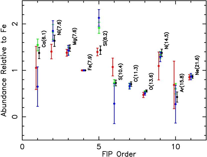
One might be a little concerned that the abundances derived from individual analyses of RGS and HETGS data do not agree with each other within the stated uncerainties. However, as we have already pointed out earlier, this is mainly the result of a weak continuum, which makes the absolute determination of abundances difficult. The uncertainties in our measurements are obtained by taking the variance along the MCMC chain in equilibrium. However, as we discussed earlier, we do not iterate the overall normalization parameter, , in our analysis. Therefore it is not surprising to see very different absolute abundance values from different analyses. The relative abundances are still well constrained in our method. In Figure 8, we plot the same data of Figure 7 with abundances measured relative to that of Fe. It is seen that measurements from different data sets are generally consistent with each other. Si is the only exception, where the RGS derived value is significantly larger than that from HETGS. We atrribute this difference to the RGS calibration problems near the Si K-shell lines.
7 Chandra LETGS
Since the Chandra LETGS data has even longer wavelength coverage than the RGS, we would expect that it provides even more stringent constraints on the low temperature DEM. However, the atomic data beyond about 40 Å is not as well known as those at shorter wavelengths, and it is possible that the LETGS effective area calibration may be problematic at longer wavelengths. This may be partially blamed for the large discrepancies found between the theoretical and observed ratios of EUV to X-ray line intensities of Fe XVIII and XIX discovered by Desai et al. (2005), which we will discuss later in more detail. Another complication of fitting the LETGS raw spectra is that its wavelengths scale is not as well determined as for RGS and HETGS because of the non-linearity of the HRC-S detector. Therefore, a better method for analyzing the LETGS data is to first identify and measure strong lines, which can then be used for DEM analysis. Argiroffi et al. (2003) adopted such an approach and used an MCMC DEM deconvolution method which is different from the one we developed here. Their derived DEM and abundances are quite similar to our results derived from the joint fit of HETGS and RGS data. However, because only a limited set of unblended lines can be used in their method, the associated uncertainties on abundances are much larger than our determination.
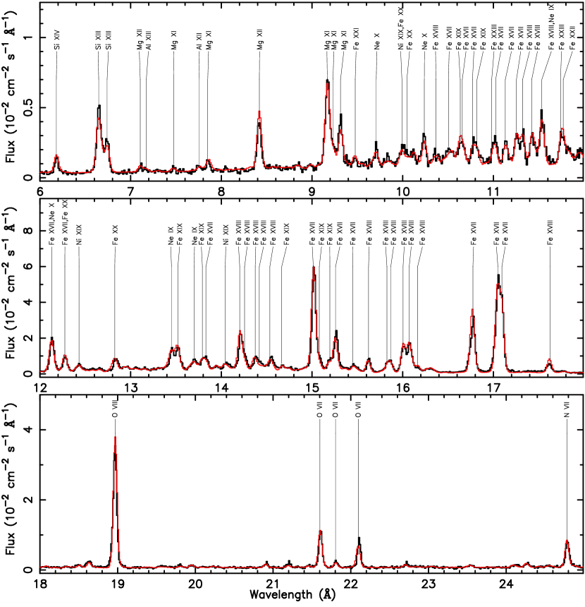
Due to the lack of variability of the Capella emission, we expect the model derived from the RGS and HETGS data to fit the LETGS X-ray spectra equally well. In the present analysis, we simply verify that this is the case without carrying out a full DEM analysis on the LETGS data. By folding the RGS and HETGS joint fit model through the LETGS response, we show the comparison of the calculated and observed spectra in Figure 11 for the wavelength region between 6 and 25 Å. It is clear that the model is a very good representation of all significant line and continuum emission.
Such good agreement is lost for wavelengths above 40 Å, as we have noted that the theoretical atomic data may be more uncertain, and there may be emission regions with lower temperatures which are not constrained by either RGS or HETGS. In the present work, we do not investigate the many discrepancies found in the long wavelength range. However, we further study the problem identified by Desai et al. (2005), i.e., the observed intensity ratios of EUV to X-ray lines of Fe XVIII and XIX are found to be a factor of 2 smaller than calculations. Here we expand the analysis to include more Fe L-shell ions.
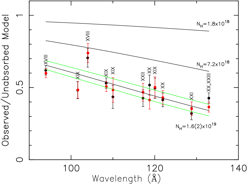
In Table 3, we list the measured and modeled fluxes of several lines in the 90 – 140 Å region, where most EUV lines of Fe ions are located. These lines all originate from the transitions of L-shell ions. It is clear that all lines are overestimated in the model by at least a factor of two. Extracting the individual line intensities in the data and the unabsorbed model, we plot the ratio as a function of wavelength in Figure 12. A total of 11 line features from Fe XVIII–XXIII are used, some of them are blends of more than one line, in which case the model intensity includes all contributions. The correction factor due to the interstellar absorption corresponding to the neutral hydrogen column density of cm-2 is also shown, which is a very small effect. The data points suggest a trend as if the absorption column density is much higher, assuming that the LETGS calibration at these wavelengths relative to the X-ray band is correct. The effective must be increased to cm-2 in order to explain the observed data.
The neutral hydrogen column density of cm-2 is measured using the interstellar absorption profile of the hydrogen Ly line toward Capella, and has a very small uncertainty (Linsky et al., 1993). However, the hydrogen ionization fraction of the local intersetallar cloud is quite uncertain. Because the absorption model used in our analysis and that of Desai et al. (2005) assumes that the interstellar medium is cold and neutral with standard cosmic abundances for all elements, the true neutral hydrogen column density may not represent all of the absorbing materials. At the wavelength region of interest, the most important contributors of absorption are H I, He I, and He II. There are considerable evidences that hydrogen and helium in the local interstellar cloud are partially ionized with a H II fraction of 0.3–0.8 (Wood et al., 2002). The detailed photoionization model of Slavin & Frisch (2002) gives the H II fraction of 0.2–0.3, and He II fraction of 0.3–0.5 with little He III. Let us define an effective neutral hydrogen column density, for a partially ionized medium, such that the absorption at certain photon energy in this medium is the same as a neutral one with column density equal to , i.e.,
| (3) |
where is the cosmic He abundance. Assuming that the H II fraction is X(H), He II fraction is X(He), and no He III,
| (4) |
For photoabsoption cross sections near 100 Å, , and , and therefore
| (5) |
where we have used . Clearly, it depends strongly on but weakly on . Assuming the average value of and cm-2, one requires in order to obtain cm-2. This H II fraction is outside the range estimated by Wood et al. (2002), which is based on the measurement of number densities of neutral hydrogen and electrons. Taking the most extreme value of from the observation would imply cm-2, which is only enough to account for about half of the discrepancies. To explain the remaining disagreement, one must assume that either the theoretical ratios of EUV to X-ray lines of Fe L-shell ions are too large by about 50%, the LETG effective area calibration is off by the same amount, or the combination of both. Either of these cases seems plausible, especially the last one, since one would only need to assume systematic errors of 20–30% in both factors.
8 Discussion and Conclusions
During this reanalysis of Capella data, we developed a new atomic line list based on APED/APEC. The improvements include better ionization balance calculations for all L-shell ions, more level population mechanisms for Fe L-shell ions such as resonance excitation, recombination, and ionization processes, better wavelengths based on either accurate many-body perturbation theory or laboratory measurements for L-shell lines of S, Ar, Fe, and Ni. We have tested the new line database on many other coronal sources, and found it to always perform better than APED/APEC. However, there are still some serious deficiencies in the atomic data. For example, the L-shell lines of elements other than Fe only include direct excitation as the level population mechanism; the line emissivities are calculated in the low density limit; and the wavelengths of high- transitions of Fe L-shell ions have not been well determined as those of transitions. Some of these problems are being addressed with the ongoing laboratory and theoretical work. We expect to further improve the database in the near future.
We also developed a new MCMC based DEM deconvolution method. It is different from existing methods in several aspects, including the parameterization of DEM and the utilization of the raw spectra instead of line fluxes. We demonstrated that the HETGS data alone often cannot constrain the total emission measure and the absolute abundances independently due to the lack of significant continuum emission. The DEM derived from RGS alone often has a high temperature tail which may bias the abundance measurements. The combination of HETGS and RGS data were shown to give the most robust results. The abundances derived from the joint analysis of HETGS and RGS indicate the presence of solar-like FIP effect.
We investigated the problem of intensity ratios of EUV lines to X-ray lines of Fe L-shell ions using the LETGS data. The overestimation of lines are shown to exist not only for Fe XVIII and XIX, but also for higher charge ions up to Fe XXIII. The discrepancy appears to grow larger for lines at longer wavelengths. We proposed a partial explanation by assuming that the interstellar medium along the Capella line sight is partially ionized, and therefore has a larger effective absorption column density than if the medium is neutral. However, constraints on the ionization fraction of H II dictate that it can only account for about half of the discrepancy. It is plausible that the remaining discrepancy is due to either the LETGS calibration uncertainties or systematic errors in theoretical line ratios.
References
- Anders & Grevesse (1989) Anders, E. & Grevesse, N. 1989, Geochim. Cosmochim. Acta, 53, 197
- Argiroffi et al. (2003) Argiroffi, C., Maggio, A., & Peres, G. 2003, A&A, 404, 1033
- Audard et al. (2001) Audard, M. et al. 2001, A&A, 365, L329
- Audard et al. (2003) Audard, M., Güdel, M., Sres, A., Raassen, A. J. J., & Mewe, R. 2003, A&A, 398, 1137
- Behar et al. (2001) Behar, E., Cottam, J., & Kahn, S. M. 2001, ApJ, 548, 966
- Brickhouse et al. (2000) Brickhouse, N. S., Dupree, A. K., Edgar, R. J., Liedahl, D. A., Drake, S. A., White, N. E., & Singh, K. P. 2000, ApJ, 530, 387
- Brinkman et al. (2000) Brinkman, A. C. et al. 2000, ApJ, 530, L111
- Brown et al. (1998) Brown, G. V., Beiersdorfer, P., Liedahl, D. A., Widmann, K., & Kahn, S. M. 1998, ApJ, 502, 1015
- Brown et al. (2002) Brown, G. V., Beiersdorfer, P., Liedahl, D. A., Widmann, K., Kahn, S. M., & Clothiaux, E. J. 2002, ApJS, 140, 589
- Canizares et al. (2000) Canizares, C. A. et al. 2000, ApJ, 539, L41
- Desai et al. (2005) Desai, P. et al. 2005, ApJ, 625, L59
- Doron & Behar (2002) Doron, R. & Behar, E. 2002, ApJ, 574, 518
- Dupree et al. (1993) Dupree, A. K., Brickhouse, N. S., Doschek, G. A., Green, J. C., & Raymond, J. C. 1993, ApJ, 418, L41
- Gu (2003a) Gu, M. F. 2003a, ApJ, 582, 1241
- Gu (2003b) —. 2003b, ApJ, 590, 1131
- Gu (2005) —. 2005, ApJS, 156, 105
- Hummel et al. (1994) Hummel, C. A., Armstrong, J. T., Quirrenbach, A., Buscher, D. F., Mozurkewich, D., & Elias, N. M. 1994, AJ, 107, 1859
- Kashyap & Drake (1998) Kashyap, V. & Drake, J. J. 1998, ApJ, 503, 450
- Lepson et al. (2003) Lepson, J. K., Beiersdorfer, P., Behar, E., & Kahn, S. M. 2003, ApJ, 590, 604
- Lepson et al. (2005) —. 2005, ApJ, 625, 1045
- Linsky et al. (1993) Linsky, J. L. et al. 1993, ApJ, 402, 694
- Manset et al. (2000) Manset, N., Veillet, C., & Crabtree, D., eds. 2000, 591
- Mazzotta et al. (1998) Mazzotta, P., Mazzitelli, G., Colafrancesco, S., & Vittorio, N. 1998, A&AS, 133, 403
- Mewe et al. (2001) Mewe, R., Raassen, A. J. J., Drake, J. J., Kaastra, J. S., van der Meer, R. L. J., & Porwuet, D. 2001, A&A, 368, 888
- Peterson et al. (2006) Peterson, J. R., Marshall, P. J., & Andersson, K. 2006, ApJ, submitted
- Phillips et al. (2001) Phillips, K. J. H., Mathioudakis, M., Huenemoerder, D. P., Williams, D. R., Phillips, M. E., & Keenan, F. P. 2001, MNRAS, 325, 1500
- Slavin & Frisch (2002) Slavin, J. D. & Frisch, P. C. 2002, ApJ, 565, 364
- Smith et al. (2001) Smith, R. K., Brickhouse, N. S., Liedahl, D. A., & Raymond, J. C. 2001, ApJ, 556, 91
- Wood et al. (2002) Wood, B. E., Redfield, S., Linsky, J. L., & Sahu, M. S. 2002, ApJ, 581, 1168
| RGSaaReconstruction from the RGS data alone. | RGS-LbbReconstruction from the RGS data alone and exlucding intermediate-Z L-shell lines. | HETGSccReconstruction from the HETGS data alone. | RGS+HETGSddReconstruction from the joint RGS and HETGS data. | |
|---|---|---|---|---|
| 5.825 | 2.43(1.11) | 2.55(1.44) | 8.67(3.86) | 1.24(1.04) |
| 5.875 | 1.63(1.01) | 1.98(1.30) | 7.94(3.60) | 1.00(0.91) |
| 5.925 | 0.90(0.78) | 1.20(0.93) | 7.40(3.62) | 0.57(0.67) |
| 5.975 | 0.46(0.57) | 0.60(0.66) | 6.47(3.51) | 0.36(0.59) |
| 6.025 | 0.31(0.48) | 0.26(0.44) | 5.12(3.18) | 0.29(0.51) |
| 6.075 | 0.26(0.45) | 0.14(0.32) | 3.97(2.73) | 0.22(0.42) |
| 6.125 | 0.23(0.42) | 0.07(0.24) | 2.65(2.29) | 0.27(0.47) |
| 6.175 | 0.33(0.50) | 0.09(0.26) | 1.67(1.90) | 0.41(0.59) |
| 6.225 | 0.56(0.57) | 0.19(0.38) | 1.32(1.65) | 0.59(0.67) |
| 6.275 | 0.87(0.76) | 0.65(0.63) | 1.27(1.71) | 1.20(0.93) |
| 6.325 | 1.16(0.81) | 1.30(0.85) | 1.74(1.88) | 1.92(1.08) |
| 6.375 | 1.45(0.98) | 2.33(1.12) | 3.02(2.45) | 1.68(1.15) |
| 6.425 | 1.66(1.05) | 3.10(1.44) | 6.22(3.65) | 1.54(1.02) |
| 6.475 | 1.27(0.95) | 2.48(1.40) | 8.74(3.63) | 1.46(1.05) |
| 6.525 | 1.41(1.03) | 2.01(1.19) | 11.32(4.38) | 1.71(1.09) |
| 6.575 | 2.31(1.33) | 1.93(1.17) | 10.74(4.38) | 2.91(1.47) |
| 6.625 | 3.55(1.42) | 2.38(1.27) | 10.71(4.31) | 4.40(1.75) |
| 6.675 | 5.10(1.73) | 3.90(1.65) | 10.39(4.39) | 6.76(2.13) |
| 6.725 | 6.02(1.87) | 5.81(1.87) | 11.43(4.64) | 8.17(2.37) |
| 6.775 | 6.89(2.09) | 7.75(2.12) | 13.49(4.64) | 8.37(2.42) |
| 6.825 | 7.18(2.06) | 7.92(2.14) | 15.76(5.08) | 8.65(2.56) |
| 6.875 | 6.99(1.88) | 7.24(2.16) | 19.25(5.36) | 9.55(2.38) |
| 6.925 | 6.83(1.83) | 6.21(1.97) | 18.90(4.97) | 9.27(2.43) |
| 6.975 | 6.17(1.73) | 5.89(1.80) | 14.00(4.36) | 7.77(2.11) |
| 7.025 | 3.48(1.32) | 3.37(1.37) | 9.12(3.60) | 4.57(1.74) |
| 7.075 | 1.18(0.85) | 1.46(0.96) | 5.76(2.83) | 2.02(1.25) |
| 7.125 | 0.55(0.58) | 0.72(0.67) | 3.01(2.29) | 1.34(0.93) |
| 7.175 | 0.32(0.50) | 0.41(0.55) | 1.49(1.49) | 1.14(0.89) |
| 7.225 | 0.34(0.50) | 0.23(0.41) | 0.51(0.95) | 0.79(0.77) |
| 7.275 | 0.42(0.55) | 0.29(0.47) | 0.17(0.59) | 0.72(0.74) |
| 7.325 | 0.36(0.52) | 0.36(0.52) | 0.01(0.18) | 0.56(0.67) |
| 7.375 | 0.37(0.55) | 0.39(0.54) | 0.00(0.00) | 0.34(0.54) |
| 7.425 | 0.40(0.56) | 0.35(0.54) | 0.00(0.00) | 0.26(0.50) |
| 7.475 | 0.41(0.56) | 0.43(0.59) | 0.00(0.00) | 0.27(0.49) |
| 7.525 | 0.53(0.62) | 0.58(0.68) | 0.00(0.00) | 0.32(0.54) |
| 7.575 | 0.77(0.78) | 0.89(0.80) | 0.00(0.00) | 0.36(0.57) |
| 7.625 | 1.22(0.96) | 1.17(1.00) | 0.00(0.00) | 0.52(0.67) |
| 7.675 | 1.82(1.14) | 1.69(1.15) | 0.00(0.00) | 0.55(0.66) |
| 7.725 | 2.46(1.26) | 2.46(1.39) | 0.00(0.00) | 0.74(0.78) |
| 7.775 | 3.90(1.48) | 3.69(1.48) | 0.00(0.00) | 0.99(0.81) |
| FIPaaFirst ionization potential. (eV) | RGSbbReconstruction from the RGS data alone. | RGS-LccReconstruction from the RGS data alone and exlucding intermediate-Z L-shell lines. | HETGSddReconstruction from the HETGS data alone. | RGS+HETGSeeReconstruction from the joint RGS and HETGS data. | |
|---|---|---|---|---|---|
| 6 | 11.3 | 0.69(0.05) | 0.68(0.06) | 0.57(0.04) | |
| 7 | 14.5 | 1.38(0.08) | 1.33(0.11) | 0.49(0.05) | 1.10(0.06) |
| 8 | 13.6 | 0.56(0.02) | 0.52(0.04) | 0.21(0.08) | 0.45(0.02) |
| 10 | 21.6 | 0.89(0.04) | 0.90(0.07) | 0.38(0.02) | 0.69(0.03) |
| 12 | 7.6 | 1.47(0.08) | 1.48(0.11) | 0.62(0.04) | 1.19(0.06) |
| 14 | 8.2 | 1.98(0.12) | 2.20(0.18) | 0.62(0.08) | 1.15(0.07) |
| 16 | 10.4 | 0.76(0.07) | 0.29(0.44) | 0.48(0.12) | 0.58(0.05) |
| 18 | 15.8 | 0.63(0.12) | 0.28(0.42) | 0.31(0.07) | 0.34(0.09) |
| 20 | 6.1 | 1.60(0.13) | 0.67(0.44) | 0.47(0.12) | 1.10(0.10) |
| 26 | 7.9 | 1.03(0.03) | 1.03(0.08) | 0.45(0.13) | 0.80(0.03) |
| 28 | 7.6 | 1.88(0.16) | 1.91(0.23) | 0.63(0.03) | 1.31(0.10) |
| Ion | (Å) | Flux (photons cm-2 ks-1) | ||
|---|---|---|---|---|
| order | order | ModelaaThe model fluxes are derived from the DEM and abundances reconstructed from the joint fit of HETGS and RGS data without including corrections due to interstellar absorption. | ||
| Fe XVIII | 94.0 | 3.96(0.10) | 3.83(0.10) | 6.40 |
| Fe XIX | 101.6 | 0.90(0.05) | 0.90(0.05) | 1.86 |
| Fe XVIII | 104.0 | 1.65(0.08) | 1.73(0.08) | 2.33 |
| Fe XIX | 108.4 | 2.98(0.10) | 2.86(0.10) | 5.63 |
| Fe XIX | 110.0 | 0.41(0.04) | 0.46(0.04) | 0.95 |
| Fe XXII | 117.2 | 0.78(0.05) | 0.85(0.06) | 1.82 |
| Fe XX | 118.8 | 0.80(0.05) | 0.64(0.05) | 1.56 |
| Fe XIX | 120.1 | 0.75(0.05) | 0.76(0.05) | 1.51 |
| Fe XX | 121.9 | 1.26(0.07) | 1.31(0.08) | 3.04 |
| Fe XXI | 128.8 | 1.28(0.09) | 1.41(0.10) | 4.00 |
| Fe XX,XXIII | 132.9 | 3.22(0.14) | 2.76(0.13) | 7.56 |
