$K$-corrections and filter transformations
in the ultraviolet, optical, and near infrared

Abstract

Template fits to observed galaxy fluxes allow calculation of $K$-corrections and conversions among observations of galaxies at various wavelengths. We present a method for creating model-based template sets given a set of heterogeneous photometric and spectroscopic galaxy data. Our technique, non-negative matrix factorization, is akin to principle component analysis (PCA), except that it is constrained to produce nonnegative templates, it can use a basis set of models (rather than the delta function basis of PCA), and it naturally handles uncertainties, missing data, and heterogeneous data (including broad-band fluxes at various redshifts). The particular implementation we present here is suitable for ultraviolet, optical, and near-infrared observations in the redshift range $0<z<1.5$. Since we base our templates on stellar population synthesis models, the results are intepretable in terms of approximate stellar masses and star-formation histories. We present templates fit with this method to data from GALEX, Sloan Digital Sky Survey spectroscopy and photometry, the Two-Micron All Sky Survey, the Deep Extragalactic Evolutionary Probe and the Great Observatories Origins Deep Survey. In addition, we present software for using such data to estimate $K$-corrections and stellar masses.

1 Motivation

New surveys at low and high redshift have provided us with estimates of galaxy spectral energy distributions (SEDs) for an enormous number of galaxies. When comparing populations of galaxies at different redshifts in these surveys, we need to use comparable measurements of the galaxy SEDs. However, different surveys use different bandpasses and the restframe wavelengths of these bandpasses necessarily vary with redshift. We need to be able to handle this heterogeneity in order to make sensible comparisons among all of these new surveys.

In this paper, we present a method for doing so, by calculating $K$-corrections between observed and desired bandpasses. The $K$-correction between a bandpass $R$ used to observe a galaxy at redshift $z$ and the desired bandpass $Q$ is defined by the equation (Oke & Sandage 1968; Hogg et al. 2002):

$$m_{R}=M_{Q}+\mathrm{DM}(z)+K_{QR}(z)-5\log_{10}h$$ (1)

where $\mathrm{DM}(z)=25-5\log_{10}(d_{L}/(h^{-1}{\mathrm{~{}Mpc}}))$ is the bolometric distance modulus calculated from the luminosity distance $d_{L}$, and $M_{Q}$ is the absolute magnitude. The absolute magnitude is defined as the apparent magnitude an object would have if were observed 10 pc away, in bandpass $Q$, at rest. The traditional definition of the $K$-correction takes $Q=R$. However, we note that in practice many surveys do perform $K$-corrections from one observed bandpass $R$ to another bandpass $Q$ in the rest frame. This practice is particularly common when dealing with high redshift observations. In addition to $K$-corrections, this method also provides an interpretation of the data in terms of a physical model which describes the stellar mass and star-formation history of each galaxy.

The method is designed to work well for a wide range of data sets. It uses photometry and spectroscopy of the Sloan Digital Sky Survey (SDSS; York et al. 2000) the Galaxy Evolution Explorer (GALEX; Martin et al. 2005) in the ultraviolet, and the Two-Micron All Sky Survey (2MASS; Skrutskie et al. 1997) in the near infrared (NIR). In addition, at higher redshifts, we use constraints from the Deep Extragalactic Evolutionary Probe 2 (DEEP2; Davis et al. 2003; Faber et al. 2003) and the Great Observatories Origins Deep Survey (GOODS; Giavalisco et al. 2004). These and other data sets provide a huge set of information about galaxy colors and spectra which we can use to help understand their star-formation histories.

We note that some of the algorithmic techniques used here may have applications in other areas of astrophysics. First, nonnegative matrix factorization (NMF; Lee & Seung 2000), and the extensions to it we describe here, is a particularly useful variant on principal component analysis. Second, the nonnegative least squares algorithm of Sha et al. (2002) has the virtue of being extremely simple to implement. These methods may find other applications in image analysis, spectroscopic analysis, and model fitting in astrophysics.

We also release the templates in electronic form as well as an implementation of the methods used to fit the templates to data. This software kcorrect v4_1 is distributed on the World Wide Web. It consists of a core C library which performs most of the complex and computationally intensive tasks, plus an IDL library that provides a high-level interface. This software is an update of two major earlier releases (v1_16; Blanton et al. 2003; v3_2). The improvement over the previous version is twofold. First, we have improved the templates such that they successfully fit galaxies in the restframe UV, as observed by GALEX, DEEP2, and GOODS. Second, because the templates are now completely model-based, the fits have a physical interpretation in terms of a star-formation history. The IDL library also has a number of new useful functions.

In Section 2, we describe how to find suitable templates, given a set of models and a set of data. We also describe the data and models used here. In Section 3, we show the results: the best-fit templates and how well they fit the data. In Section 4, we describe how to convert our results into an estimate of the $K$-correction. In Section 5, we describe the physical interpretation of the templates and of fits to data. In Section 6, we present some simplified, linear transformations between various bandpasses. In Section 7, we summarize our results. Appendix A describes the NMF algorithm. Appendix B describes the electronic format of our results.

Where necessary, we have assumed cosmological parameters $\Omega_{0}=0.3$, $\Omega_{\Lambda}=0.7$, and $H_{0}=100$ $h$ km s^-1 Mpc^-1 (with $h=1$), unless otherwise noted. All magnitudes are (unless otherwise noted) AB-relative. Except where noted, I will always be referring to the version of the kcorrect software labeled v4_1_4.

2 Finding the templates

2.1 Overview

From the spectroscopic observations we know that galaxy spectra reside in a low-dimensional subspace. Principal Component Analysis (PCA) of galaxy spectra, introduced by Connolly et al. (1995) and applied many times since then, demonstrates that most of the variance in the distribution of galaxies in spectral space can be explained using a few templates. This means that, in the linear space of all possible spectra, galaxies exist in only a small subspace. Therefore, even with very heterogeneous data, we should be able to determine the properties of this subspace.

Here we present an approach to combining heterogeneous data in order to determine the properties of the subspace of galaxy spectra. Rather than taking the model-free approach used by PCA, we here restrict the space of possible spectra to those predicted from the high resolution stellar population synthesis model of Bruzual & Charlot (2003) and the nebular emission line models of Kewley et al. (2001). This approach both constrains the problem appropriately and yields a natural theoretical interpretation of the results in terms of star-formation histories.

In a nutshell, our algorithm does the following. Given the observations (and uncertainties of those observations) available for each galaxy, it finds the nonnegative linear combination of $N$ template star-formation histories which best predict those observations in the $\chi^{2}$ sense. Given the entire set of galaxy observations available, it also fits for the $N$ template star-formation histories. The technical name for this algorithm is Nonnegative Matrix Factorization (NMF; Lee & Seung 1999, 2000), and we describe it in detail in Appendix A. Note that this problem is not the same as the well-known nonnegative least squares problem, which would fit for the best-fit nonnegative linear combination of templates, but not for the form of the templates themselves.

This approach is similar to PCA in that it finds the small spectral subspace in which galaxies exist, and can in some ways be thought of as “nonnegative PCA.” However, our method has several advantages over the standard PCA approach. First, the results yield, along with a subspace in the space of all possible spectra, a natural interpretation, which is the corresponding subspace in the space of all possible star-formation histories. Second, it naturally handles data uncertainties and missing data, which allows it to ignore that variation which is due purely to statistical errors. Third, it handles the complications of observing galaxy spectra photometrically using broad-band filters of galaxies at varying redshifts, whereas standard PCA requires a constant grid of observations in rest-frame wavelength space.

In the following subsections, we introduce the basis set of models we use here (§2.2), the data we fit to (§2.3), and how we combine the two to set up the NMF problem (§2.4). In Appendix A we describe how to actually solve to NMF problem.

2.2 The models

We begin with a basis set of 485 spectral templates. Of these, 450 are a set of instantaneous bursts from Bruzual & Charlot (2003), using the Chabrier (2003) stellar initial mass function and the Padova1994 isochrones. We select 6 metallicities (0.005, 0.02, 0.2, 0.4, 1, and 2.5 times solar). For each metallicity we select 25 ages (between 1 Myr and 13.75 Gyr, spaced almost logarithmically in age). For each age and metallicity we make 3 choices of dust model: (1) no dust extinction; (2) $\tau_{V}=3$ dust with Milky Way type extinction (as input into the models of Witt & Gordon 2000 with a “homogeneous” distribution and “shell” geometry); (3) $\tau_{V}=3$ dust with SMC type extinction (from the same models). We smooth each template to $300$ km s^-1 velocity dispersion (we will smooth the SDSS spectra in the training set to the same resolution).

The remaining 35 templates are from MAPPINGS-III (Kewley et al. 2001) models of emission from ionized gas. We choose the predictions for an 8 Myr old continuous star-formation history with 5 possible metalliciticites (0.5, 0.2, 0.4, 1.0, and 2. times solar) and 7 possible ionization parameters ($q=5\times 10^{6}$, $10^{7}$, $2\times 10^{7}$, $4\times 10^{7}$, $8\times 10^{7}$, $1.5\times 10^{8}$, and $3\times 10^{8}$ cm s^-1). We take the spectra (given as a set of delta functions) and smooth them to $300$ km s^-1 velocity dispersion. The one alteration we make to all of these templates is to remove Ly$\alpha$, because it is generally much larger than observed in real galaxies.

Let us refer to these 485 basis templates as $M_{j}(\lambda)$, expressed in units of ergs s^-1 A^-1.

We seek to reduce this full basis space to a subspace in which galaxies actually exist. In particular, we seek five templates $F_{i}(\lambda)$ built from nonnegative combinations of the original basis set of $N$ templates:

$$F_{i}(\lambda)=\sum_{j}b_{ij}M_{j}(\lambda),$$ (2)

in units of ergs s^-1 A^-1. In principle, we could seek any number of templates; from our experiments, we have found that five turns out to be a number large enough to explain the data we use here. For each galaxy $k$ we want our model ${\hat{F}_{\lambda}}(\lambda)$ for their spectrum to be a nonegative sum of these five templates:

$${\hat{F}}_{k}(\lambda)=\sum_{i}a_{ki}F_{i}(\lambda).$$ (3)

2.3 The data

The training set consists of:

1. SDSS spectroscopic data in the observed range $3800<\lambda<9000$ A, for 400 Luminous Red Galaxies between $0.15<z<0.5$ (LRGs; Eisenstein et al. 2001) and 1600 Main sample galaxies between $0.001<z<0.4$ (Strauss et al. 2002)

2. SDSS photometric data on an independent set of LRGs ($griz$ photometry only) and Main sample galaxies (using the full $ugriz$ photometry) in the same redshift ranges. We use 2000 LRGs and 7000 Main sample galaxies. For these galaxies we include 2MASS $JHK_{s}$ extended source catalog data (Jarrett et al. 2000) where available.

3. GALEX DR1 far UV ($\sim 1500$ A) and near UV ($\sim 2300$ A) photometry for Main sample SDSS galaxies with redshifts and $ugriz$ photometry (4000 galaxies; Martin et al. 2005).

4. The $BRI$ photometry for high redshift galaxies in the DEEP2 DR1 release between $0.6<z<1.5$ (4000 galaxies; Davis et al. 2003; Faber et al. 2003).

5. The $BVizJHK_{s}$ photometry for GOODS galaxies between $0.5<z<2$ (1000 galaxies; Giavalisco et al. 2004).

The SDSS, 2MASS, and GALEX galaxies were selected from and the matches were obtained by the New York University Value-Added Galaxy Catalog (NYU-VAGC; Blanton et al. 2005).

The SDSS data processing consists of astrometry (Pier et al., 2003); source identification, deblending and photometry (Lupton et al., 2001); photometricity determination (Hogg et al., 2001); calibration (Fukugita et al., 1996; Smith et al., 2002); spectroscopic target selection (Eisenstein et al., 2001; Strauss et al., 2002; Richards et al., 2002); spectroscopic fiber placement (Blanton et al., 2003); and spectroscopic data reduction. We recalibrated our photometry using the “ubercalibration” procedure described in Blanton et al. (2005). Descriptions of these pipelines also exist in Stoughton et al. (2002). An automated pipeline called idlspec2d (in this case v4_9) measures the redshifts and classifies the reduced spectra (Schlegel et al., in preparation). We use the Petrosian magnitudes for the SDSS data (except where noted below for the LRG-only sample).

For the GALEX and GOODS data we use “auto” magnitudes, which are the Kron-like magnitudes from SExtractor (Bertin & Arnouts 1996). For 2MASS we use the “extrapolated” magnitudes from the Extended Source Catalog (Jarrett et al. 2000).

Note that there are 20 different broadband photometric filters listed above ($B$ in DEEP2 is different than the $B$ used by GOODS). The kcorrect product described in Section 7 contains a tabulation of the response functions for all of these filters.

2.4 Comparing data and models

The data consist of spectra and bandband photometric measurements of galaxies at a number of redshifts, and we have to relate the models to these measurements.

For the spectra, we take the observed spectrum $f_{k}(\lambda)$ (in ergs cm^-2 s^-1 A^-1) of each galaxy $k$ at redshift $z$ (corresponding to a luminosity distance $d_{L}(z)$ in cm; see Hogg 1999) and calculate the restframe luminosity per unit wavelength:

$${{F}}_{k}(\lambda)={{f}}_{k}[\lambda(1+z)](1+z)(4\pi d_{L}^{2}),$$ (4)

That is, the spectrum is shifted due to the redshift, while the integral of the numerator over wavelength (the total luminosity) is constant with redshift, and the total flux is related to the total luminosity by the inverse square law. In addition, we smooth each spectrum by such an amount that, given its estimated velocity dispersion, its total velocity dispersion after smoothing is 300 km s^-1 (there are a small number of galaxies with larger velocity dispersions, which we leave unchanged).

Note that if we discretize the spectra to wavelengths $\lambda_{l}$, the relationship between the predicted SED for a galaxy $k$ and the basis set $M_{jl}$, becomes simply:

$$\hat{F}_{kl}=\sum_{ij}a_{ki}b_{ij}M_{jl}$$ (5)

If one has a spectrum for a galaxy the expression for the contribution to $\chi^{2}$ from each wavelength $\lambda_{l}$ in the spectrum is then quite simple:

$$\chi_{kl}^{2} = \left[\frac{F_{k}(\lambda_{l})-{\hat{F}}_{k}(\lambda_{l})}{\sigma^{2}_{k}(\lambda_{l})}\right]^{2}$$ (6)

$$= \left[\frac{F_{k}(\lambda_{l})-\sum_{ij}a_{ki}b_{ij}M_{jl}}{\sigma^{2}_{k}(\lambda_{l})}\right]^{2}.$$ (7)

Comparing observed broadband flux measurements is a bit more complicated, because it is a projection of the spectrum onto the broadband filter $p$ at the observed redshift $z$. Instead of adjusting the observed fluxes as we could so easily do for the spectra above, for the photometry we express the models in terms of predicted broadband fluxes at each redshift.

Here we express the flux for each galaxy $k$ in units of AB maggies $\mu_{p}$, which are defined as what one would measure in bandpass $p$ relative to the AB standard source. For example, if we transform our spectral energy density basis function $M_{j}(\lambda)$ to a flux density $m_{j}(\lambda)$, we can calculate the contribution of that basis function to the predicted maggies as:

$$\mu_{jp}=\frac{\int_{0}^{\infty}d\lambda\lambda R_{p}(\lambda){m}_{j}(\lambda)}{\int_{0}^{\infty}d\lambda\lambda R_{p}(\lambda)f_{\mathrm{AB}}(\lambda)}$$ (8)

Here, the response function $R_{p}(\lambda)$ is proportional to the contribution to the detector signal of a photon with wavelength $\lambda$ entering the Earth’s atmosphere (or entering the telescope for a space telescope). The AB standard source is $f_{\mathrm{AB}}(\lambda)d\lambda=f_{\mathrm{AB}}(\nu)d\nu$ and $f_{\mathrm{AB}}(\nu)=3631$ Jy $=3.631\times 10^{-20}$ erg s^-1 cm^-2 Hz^-1. Of course maggies $\mu$ are related to magnitudes $m$ as:

$$m=-2.5\log_{10}\mu,$$ (9)

such that the AB standard source would (if it existed) have $\mu=1$ and $m=0$ for all bandpasses.

In this context it is worth noting that many authors (e.g. Bessell 1990) tabulate the contribution to the detector signal per unit of energy in photons of wavelength $\lambda$ instead of per photon with wavelength $\lambda$. We will refer here to the former quantity as $R_{p}^{\prime}(\lambda)$, though in the literature it is often referred to without a prime (and without any explicit definition!). Clearly $R_{p}(\lambda)\propto R_{p}^{\prime}(\lambda)/\lambda$, since the higher the frequency of the photon, at a fixed response per unit energy there is a higher response per photon. With this substitution, one can reexpress Equation 8 appropriately in terms of $R_{p}^{\prime}(\lambda)$. Generally, though not universally, authors tabulate $R_{p}^{\prime}(\lambda)$ for bandpasses whose standards were originally calibrated using energy-counting devices rather than photon-counting devices. However, from the point of view of the analysis of the observations it is irrelevant what the devices used for the standards and the observations are, as long as one calculates $R_{p}(\lambda)$ and uses Equation 8.

The prediction for the broadband fluxes from Equation 8 is only for a specific redshift $z$. It turns out to simplify our mathematics to calculate the projection of each basis function $j$ onto each filter $p$ for a grid of redshifts (in this case spaced by 0.005 between redshifts 0 and 2). Thus, below we will take $p$ to index all the filters at all such redshifts.

Just as before, we can now write down the relationship between the predicted broadband flux and the basis set $\mu_{jp}$, in the bandpass and redshift corresponding to the index $p$, for a galaxy $k$:

$$\hat{\mu}_{kp}=\sum_{ij}a_{ki}b_{ij}\eta_{jp}$$ (10)

The contribution to the total $\chi^{2}$ of a broadband flux is therefore just:

$$\chi^{2}_{kp} = \left[\frac{\mu_{kp}-\hat{\mu}_{kp}}{\sigma_{kp}}\right]^{2}$$ (11)

$$= \left[\frac{\mu_{kp}-\sum_{ij}a_{ki}b_{ij}\eta_{jp}}{\sigma^{2}_{kp}}\right]^{2}.$$ (12)

For a given galaxy we do not have every filter, and we only have an observation of each filter at a single redshift. We pick the closest redshift on the redshift grid, and use the measured filters at that redshift for our expression of $\chi^{2}$, and set $1/\sigma_{kp}^{2}=0$ for the rest of the values of the index $p$ so that we zero-weight those predictions.

The matrices $\eta_{jp}$ (related to the broad-band fluxes) and $M_{jl}$ (related to the spectra) are totally fixed, and we combine them into a single matrix $M_{jn}$ and the indices $p$ and $l$ into a single index $n$, to handle both the broad-band fluxes and spectra simultaneously. We can similarly combine our observations $\mu_{kp}$ and $F_{k}(\lambda_{l})$ and their uncertainties $\sigma_{kp}$ and $\sigma_{k}(\lambda_{l})$ into vectors $x_{kn}$ and $\sigma_{kn}$. Then we can combine the Equations 6 and 11 into a single equation:

$$\chi^{2}=\sum_{kn}\left[\frac{x_{kn}-\sum_{ij}a_{ki}b_{ij}M_{jn}}{\sigma_{kn}}\right]^{2}$$ (13)

There is a simple method that we describe in Appendix A called nonnegative matrix factorization (NMF) to iterate to the nonnegative $a_{ki}$ and $b_{ij}$ which locally minimize Equation 13. The basic method is implemented in a public piece of code named NMF_SPARSE in the idlutils distribution of IDL utilities.. As the name implies, our implementation takes advantage of the fact that many of the matrix operations are on very sparse matrices (for example, for each galaxy with photometric data there are no spectroscopic data points and only photometric data at a single redshift).

As we describe in Appendix A, the NMF problem is not convex: that is, there are multiple local minima. Our method finds one of the local minima, but is not guaranteed to find the global minimum. Thus, the reader who tries to reproduce our results using our methods or others may (depending on their initial conditions) find different local minima of $\chi^{2}$ than do we.

Once we have fit for $b_{ij}$ using the training set, we can minimize Equation 13 for any other galaxy using any nonnegative least squares algorithm to determine $a_{ki}$ (since the minimization of Equation 13 has a linear form in that case). When we do so here we use the beautifully simple iterative method of Sha et al. (2002).

3 Results

3.1 An example: the Luminous Red Galaxy templates

We begin with the simplest case, which is fitting a single template to the photometric data of the LRG sample (Eisenstein et al. 2001). For many of these galaxies, which extend to $r<19.5$ and are intrinsically red, the $u$-band flux is extremely poorly measured, so we ignore the $u$-band for all LRGs.

Figure 1 shows the spectrum of the best-fit LRG. This template is constrained by data between about 2000 A and 10000 A; outside that range it is an extrapolation.

Figure 2 shows the star-formation history corresponding to this best-fit LRG spectrum. The top panel shows the star-formation per unit time as a function of look-back time. The bottom panel shows the mean metallicity of the forming stars as a function of time. When considering these plots and those below, do remember that although these results are our best-fit, the parameters are highly degenerate (especially in, for example, neighboring age bins). We show these merely to illustrate the general nature of the fits.

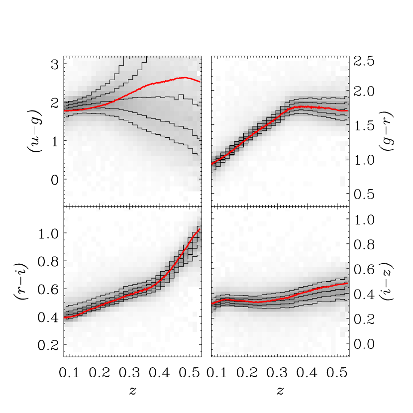
Figure 3 shows the LRG colors as a function of redshift, with the best fit template color overplotted as the smooth, thick line. In the code described in Section 7, we used the routine sdss_kcorrect (with the optional flag /lrg) to perform these fits. The best fit is a good fit to the data.

Note that in this example we have fit a nonevolving template, which is inappropriate over this range of redshifts — even if it is a good fit to the colors! In principle, we can adjust the methods used here for the case of evolving templates, but we will not do so here.

In Appendix B we describe the form in which we release the star-formation histories and spectra associated with this template.

3.2 Templates for the full data set

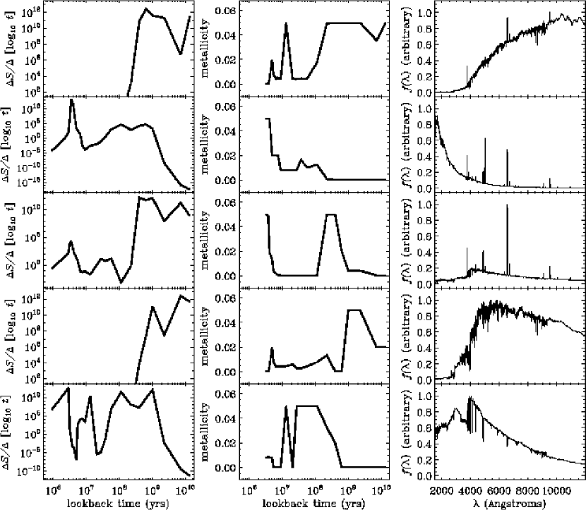
We next apply the method to the full data set and fit for five templates. From experiments, we found that we needed five to adequately explain the data. More than five templates would allow us to explain the data better, but only marginally so. The right-most column of Figure 4 shows the spectrum from the ultraviolet through the near infrared for the resulting templates. Note that there is a very old template, a very young template, and several intermediate templates, including one which is close to that of an A star.

The left and middle columns of Figure 4 show the star-formation histories and metallicities associated with the templates. We have not imposed any smoothness criterion on these fits, which explains the ragged appearance of these histories. The details of these fits are weakly constrained due to degeneracies within and among the templates, but we show them here for completeness.

In all the results below, we use these five templates, unaltered. That is, when we speak below of “fitting” the templates, we mean we fix $b_{ij}$ to the five templates shown in this section and fit only for $a_{ki}$. Since we have determined these templates to be appropriate for the data sets we include in the training set, they end up providing good fits to most other galaxies from the parent data sets. In general below, the tests we perform are not to the training set but to independent sets of galaxies.

In Appendix B we describe the form in which we release the star-formation histories and spectra associated with these templates.

3.3 Explanatory power of templates

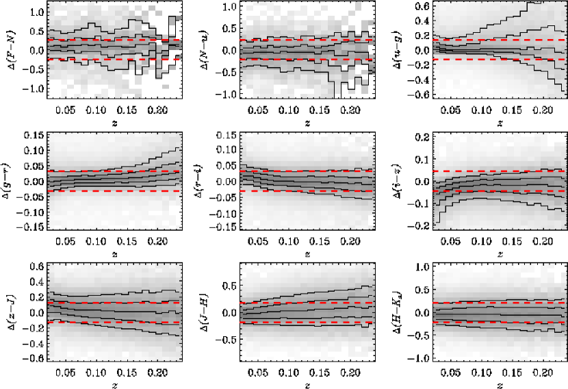
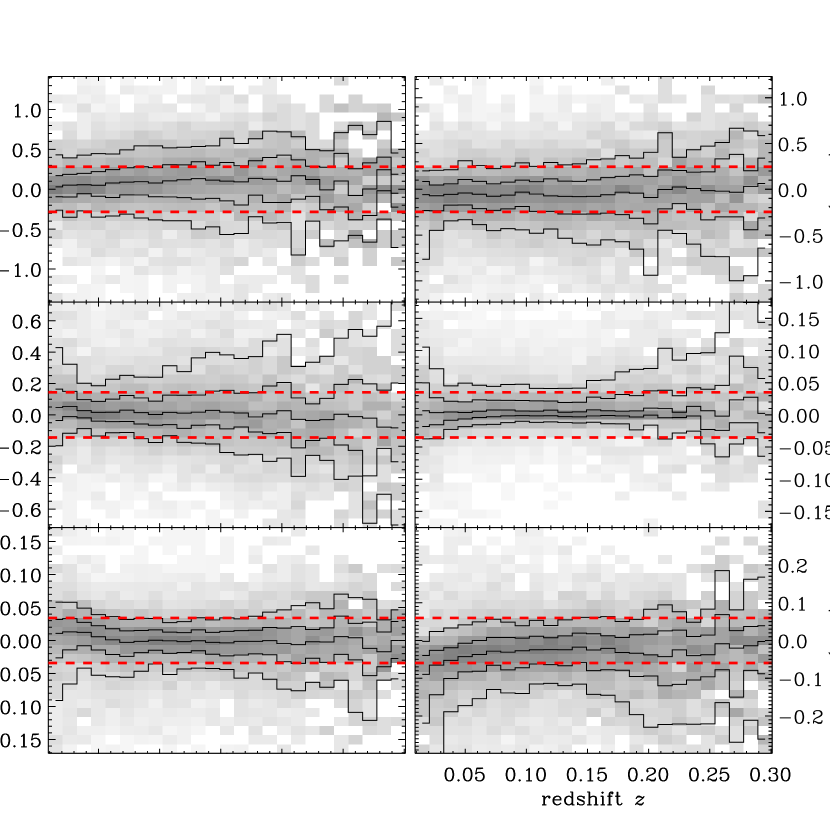
These templates explain the photometric data rather well. For example, consider Figure 5, showing the color residuals of the observations with respect to the best fits, when fitting to galaxies with GALEX, SDSS, and 2MASS data. In this context we define the color residuals as (for example):

$$\Delta[u-g]=[u_{\mathrm{obs}}-g_{\mathrm{obs}}]-[u_{\mathrm{model}}-g_{\mathrm{model}}].$$ (14)

In the code described in Section 7, we used the routine gst_kcorrect to perform these fits. In Figure 5 the thick dashed lines show the estimated 1$\sigma$ uncertainties in the colors from the photometric catalogs. Relative to the uncertainties, there are no significant biases or redshift trends in these fits. Note that the galaxies used in this test are distinct from the training set on which we fit the five templates.

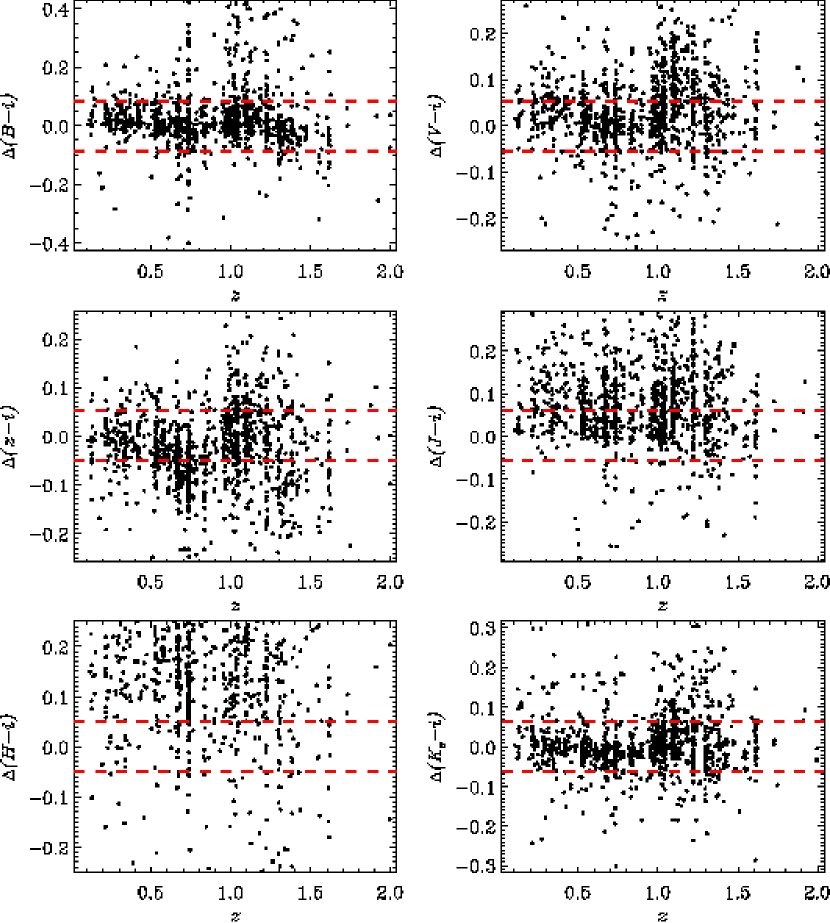
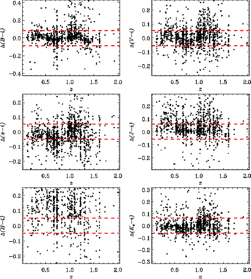
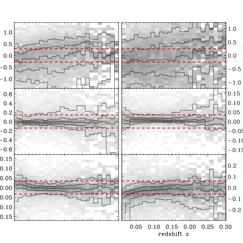
The templates do well on higher redshift data, as well. For example, Figure 6 shows the color residuals for GOODS data. Here we find that there are somewhat larger residuals with respect to the uncertainties (again shown as the thick dashed lines). We can compare this result to that in Figure 7, which we get by fitting a new set of templates to only the GOODS data (this alternate set of five templates is also distributed in the manner that Appendix B describes). From Figure 7, we conclude that some of the errors are irreducible, and require either a larger set of templates for high redshift galaxies (a possibility we find a priori unlikely), or that there are simply errors in the catalogs or the input filter curves. For example, in the $z$ and $V$ bands we find significant trends between redshifts $z=0.5$ and $1.5$ (echoed in Figure 6). More significantly, in the $H$ band there is at least a 10% offset in the magnitudes across all redshifts, which is almost certainly a catalog or filter curve error. Other errors (such as a large scatter in the residuals in the $B$ band and some redshift dependence in the $J$ band) are clearly due to the fact that the templates are not primarily designed for GOODS data. All in all, we recommend using the special templates for $K$-corrections within the GOODS data set.

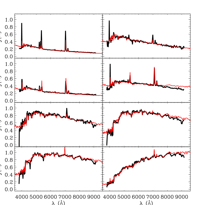
We can also test how well these templates recover actual spectra given only photometry. To do so, we take eight random SDSS spectra (chosen to span color space), project them onto the $g$, $r$ and $i$ bandpasses, and then fit the five templates to just these three fluxes. Figure 8 compares the reconstructed model spectra to the original spectrum. The two agree well in general, though some features (like the emission lines) are not reproduced well. Naturally, this success is mostly due to the quality of the original stellar spectra used in the population synthesis code of Bruzual & Charlot (2003). We are not suggesting that $gri$ photometry contains as much information as the full spectra. However, these results encourage us that by using broad-band data we can infer $K$-corrections of galaxies.

3.4 Predictive power of templates

Perhaps more interestingly, the templates do a good job of predicting missing data. That is, we can ask the question: if we use the templates to fit only to some bands but leave out others, how well do the best fits predict the bands left out?

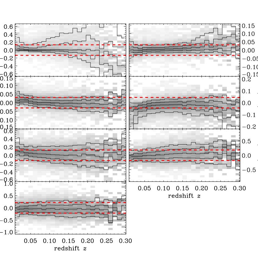
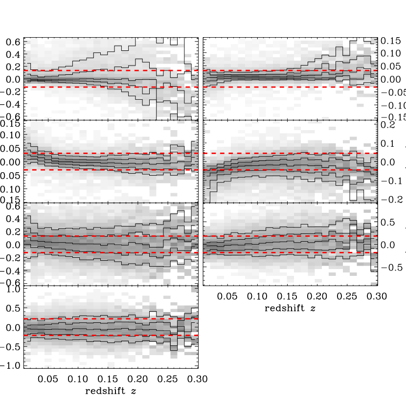
Consider Figures 9 and 10. The former shows the color residuals of fitting to both SDSS and 2MASS data for each galaxy. The latter shows the color residuals when we fit only to the SDSS data and do not include 2MASS in the fit at all. Without any input from 2MASS the templates do a very good job of predicting the 2MASS fluxes, with a scatter of 20–30% — not far from the uncertainties in the 2MASS fluxes themselves. Of course, it is not surprising that it is easy to predict the 2MASS fluxes — stellar spectra are very simple in the NIR, so having the $ugriz$-band fluxes from SDSS yields much information regarding the redder bandpasses.

However, we will note here that this result flies in the face of a persistent insistence that NIR observations are necessary to measure stellar masses of galaxies. If we can predict the NIR observations themselves, clearly they cannot be adding much to our knowledge of the underlying stellar mass. This fact changes one’s decisions about what data is best to use for calculating the stellar mass function. Basing it on 2MASS data only improves slightly the stellar mass estimate of each galaxy, while restricting (and thus biasing) the sample significantly at the lowest luminosities and surface brightnesses relative to the SDSS. Of course, if at high redshift galaxies have a very different locus of their SEDs, then perhaps this statement is less true for them.

In addition, consider Figures 11 and 12. The former shows the color residuals of fitting to both SDSS and GALEX data for each galaxy. The latter shows the color residuals when we fit only to the SDSS data and do not include GALEX in the fit at all. Without any input from GALEX the templates do a significantly worse job at predicting the GALEX fluxes. The scatter becomes about $\sigma\sim 0.5$ mag. As is common knowledge, it is more difficult to predict the UV fluxes, because dust and recent star-formation are so variable among galaxies. However, the median residuals based on are our templates still near zero.

4 Determining $K$-corrections

Given a model spectrum for the galaxy, the determination of the $K$-correction is straightforward. Here we give the relevant formulae for the $K$-corrections, leaving the derivation to Hogg et al. (2002). Then, we show the typical $K$-corrections for the data we have fit to.

The $K$-correction between a bandpass $R$ used to observe a galaxy at redshift $z$ and the desired bandpass $Q$ is defined by the equation (Oke & Sandage 1968; Hogg et al. 2002):

$$m_{R}=M_{Q}+\mathrm{DM}(z)+K_{QR}(z)-5\log_{10}h$$ (15)

where $\mathrm{DM}(z)=25-5\log_{10}(d_{L}/(h^{-1}{\mathrm{~{}Mpc}}))$ is the bolometric distance modulus calculated from the luminosity distance $d_{L}$, and $M_{Q}$ is the absolute magnitude. The absolute magnitude is defined as the apparent magnitude an object would have if were observed 10 pc away, in bandpass $Q$, at rest. The traditional definition of the $K$-correction takes $Q=R$. However, we note that in practice many surveys do perform $K$-corrections from one observed bandpass $R$ to another bandpass $Q$ in the rest frame. This practice is particularly common when dealing with high redshift observations. In addition to $K$-corrections, this method also provides an interpretation of the data in terms of a physical model which describes the stellar mass and star-formation history of each galaxy.

Equation (15) holds if the $K$-correction $K_{QR}$ is

$$K_{QR}=-2.5\,\log_{10}\left[\frac{1}{[1+z]}\,\frac{\displaystyle\int\mathrm{d}\lambda_{o}\,\lambda_{o}\,L_{\lambda}\!\left(\frac{\lambda_{o}}{1+z}\right)\,R(\lambda_{o})\,\int\mathrm{d}\lambda_{e}\,\lambda_{e}\,g^{Q}_{\lambda}(\lambda_{e})\,Q(\lambda_{e})}{\displaystyle\int\mathrm{d}\lambda_{o}\,\lambda_{o}\,g^{R}_{\lambda}(\lambda_{o})\,R(\lambda_{o})\,\int\mathrm{d}\lambda_{e}\,\lambda_{e}\,L_{\lambda}(\lambda_{e})\,Q(\lambda_{e})}\right]\;\;\;.$$ (16)

Here, $R(\lambda)$ and $Q(\lambda)$ represent the response of the instrument per unit photon entering the Earth’s atmosphere (or the telescope aperture for a space instrument). $g^{R}_{\lambda}$ is the flux density per unit wavelength (e.g.  ergs s^-1 cm^-2 A^-1) for the standard source for band $R$, and similarly for band $Q$. For example, if the magnitudes are AB relative, then these represent the AB standard source, while if they are AB relative then they represent the spectrum of Vega.

A particularly common special case is when $R=Q$:

$$K_{R}(z)=-2.5\,\log_{10}\left[\frac{1}{[1+z]}\,\frac{\displaystyle\int\mathrm{d}\lambda_{o}\,\lambda_{o}\,L_{\lambda}\!\left(\frac{\lambda_{o}}{1+z}\right)\,R(\lambda_{o})\,}{\displaystyle\int\mathrm{d}\lambda_{e}\,\lambda_{e}\,L_{\lambda}(\lambda_{e})\,R(\lambda_{e})}\right]\;\;\;.$$ (17)

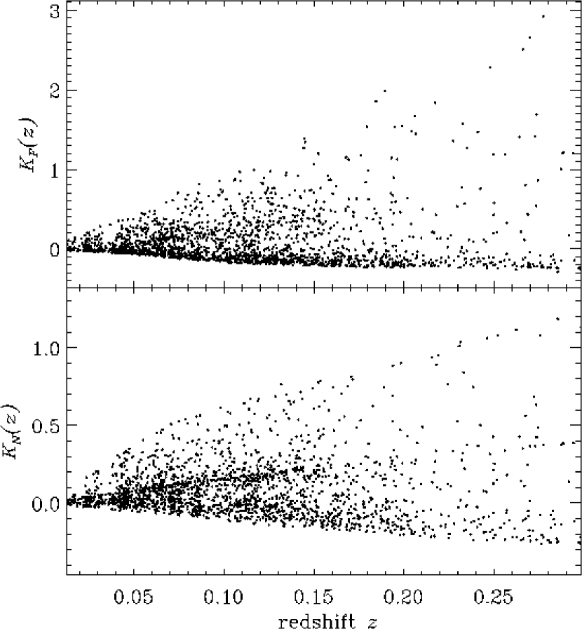
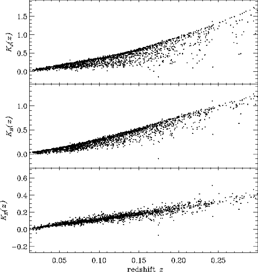
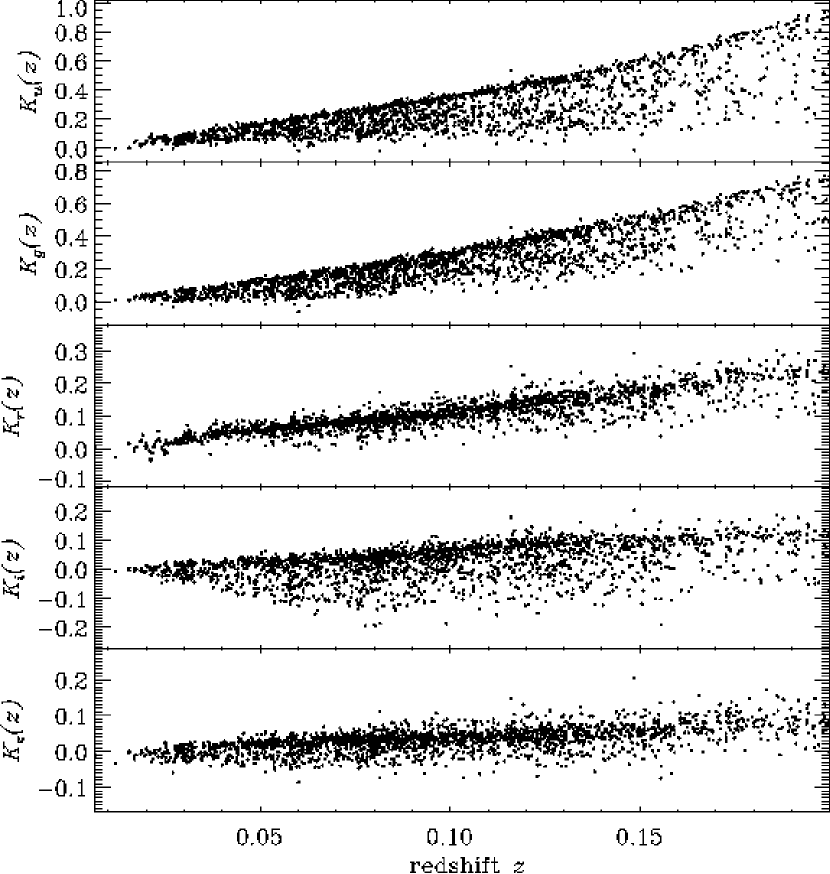
For example, consider Figures 13, 15 and 14. For a randomly selected set of galaxies these figures show the $K$-corrections from the observed frame bandpasses of GALEX, SDSS, and 2MASS respectively, to the same bandpasses in the rest frame.

Often, it makes sense to $K$-correct to a different set of band passes than the rest frame. For example, the SDSS Main sample is mostly around $z=0.1$, so it does not always make sense to $K$-correct from the observed frame $r$ band to the rest frame $r$ band. Doing so means applying large and uncertain corrections to all galaxies. If precision is not important, this uncertainty might be worth the simplification it brings. However, if one is (say) interested in the evolution of galaxies, the clustering of galaxies, or something else that requires precision, it makes more sense to avoid introducing unnecessary uncertainty.

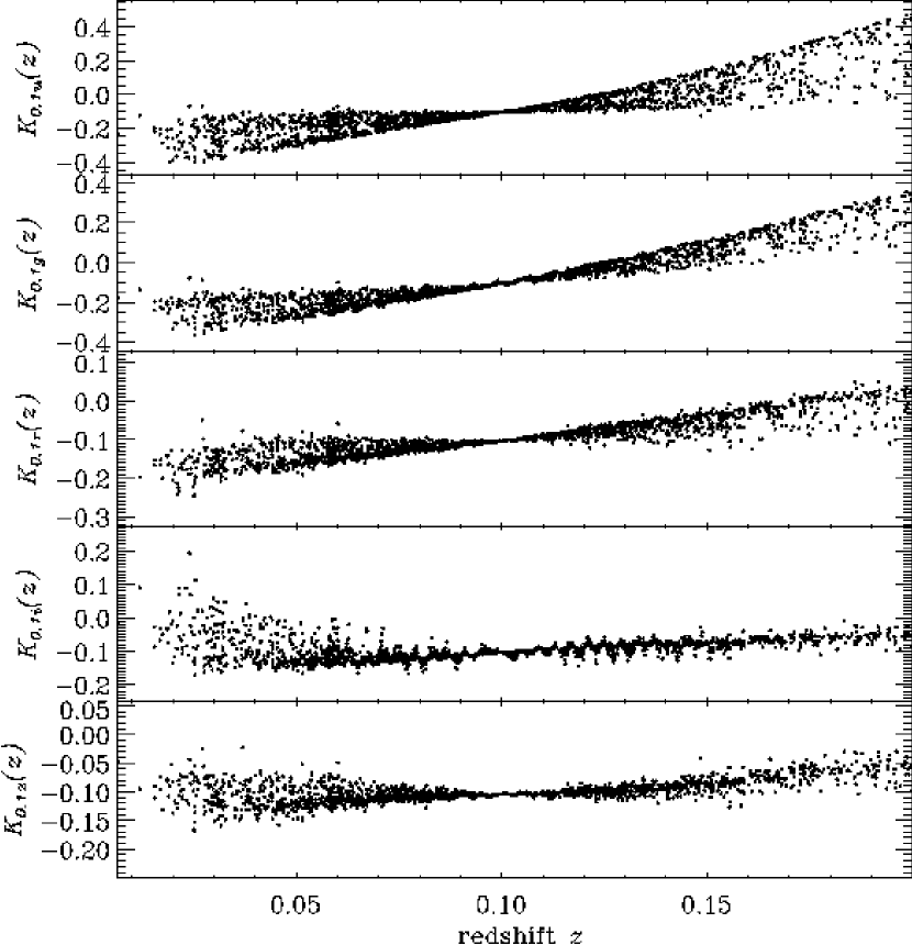
Our solution to this problem is to correct the magnitude to blue-shifted bandpasses that correspond to the observed bandpass at some intermediate redshift. We denote these bandpasses ${}^{{z}}\!{b}$, where the blue-shift in this case is by a factor $1+z$. For example, in the case of SDSS galaxies it makes sense to correct to the ${}^{{0.1}}\!{r}$ bandpass — the $r$ band blue-shifted to $z=0.1$. This bandpass has the property that the $K$-correction is independent of the SED of the galaxy. If the magnitudes are AB relative, then the $K$-correction to ${}^{{z}}\!{b}$ for a galaxy at redshift $z$ is simply $-2.5\log_{10}(1+z)$.

Figure 16 shows the $K$-corrections from the $[ugriz]$ bands to the ${}^{{0.1}}\!{[ugriz]}$ bands as a function of redshift for SDSS galaxies. Note that the $K$-corrections converge at $z=0.1$, so that around that redshift (where most galaxies are) the uncertainties in the $K$-corrections are minimized. Compare this simplicity to Figure 15, where the $K$-corrections at redshift $z=0.1$ in the $g$-band range between $0.$ and $0.2$ (and in the $u$-band from $0.$ and $0.5$). Most SDSS galaxies are near redshift $z=0.1$, and obviously the $K$-corrections are not perfect — why introduce a large uncertainty for most galaxies when it can easily be avoided?

5 Physical interpretation of the models

In addition to $K$-corrections, these template fits also provide physical interpretations of the galaxies, since they correspond to actual stellar population synthesis models. Indeed, the code outputs three parameters relevant to the star-formation history: the current mass of stars in the galaxy; the stellar mass-to-light ratio of the galaxy; and the fraction of the total amount of star-formation that has occurred recently.

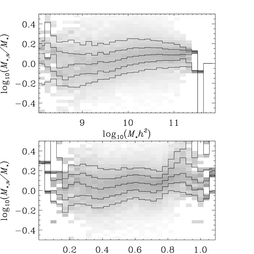
Kauffmann et al. (2003) have also calculated stellar masses for SDSS galaxies. Roughly, they have calculated the $z$-band stellar mass-to-light ratios of models which best fit the H$\delta$ absorption and D4000 measurements of the spectra, and then applied those mass-to-light ratios to the observed $z$-band luminosities of the imaging. Figure 17 shows a galaxy-by-galaxy comparison of their stellar masses $M_{\ast,s}$ relative to our $M_{\ast}$, as a function of $M_{\ast}$ and of intrinsic $g-r$ color. The two sets of masses are very similar to each other, with a scatter of only 0.1 dex and trends of less than 0.2 dex with stellar mass. To be explicit, the masses in Figure 17 correspond to the current mass in stars remaining in the galaxy. This mass can differ from the total star-formation rate integrated over time, due to the fact that stars can die — and in practice for our fits the total integrated star-formation rate is usually about twice as high as the total current mass in stars.

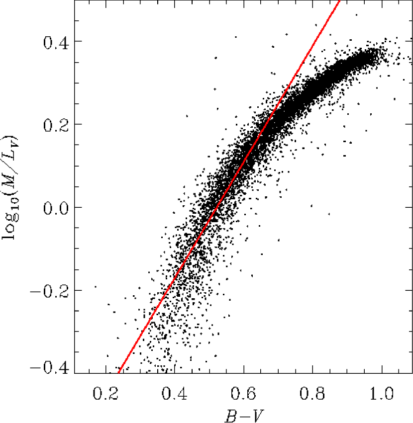
Similarly, Figure 18 shows the mass-to-light ratios of SDSS galaxies in the $V$ band as a function of color in $B-V$. Here, we have calculated the $B$ and $V$ band fluxes based on the template fits to each galaxy, as explained in Section 6 below. We give the mass-to-light ratio in solar units. The solid line is the relationship that Bell & de Jong (2001) give based on their fits to spiral galaxies. For blue galaxies ($B-V<0.8$) this line is indeed a good fit to our results. For the typical red galaxy, the Bell & de Jong (2001) relation predicts a larger stellar mass than we do.

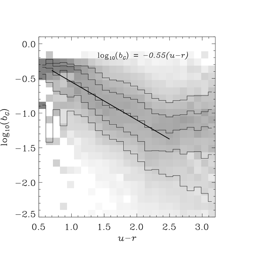
Finally, we can also calculate measures of the recent star-formation rate from these fits. Since our fits are to broad-band photometry, and not based on emission line measurements, we cannot expect to have detailed information about the very recent star-formation rate. However, we can try to measure what fraction of the total star-formation has occurred in, say, the past 1 Gyr:

$$b_{G}=\frac{\int_{0}^{1\mathrm{~{}Gyr}}dt\,\mathrm{SFR}(t)}{\int_{0}^{a_{\mathrm{Univ}}}dt\,\mathrm{SFR}(t)}$$ (18)

where the definition here is meant to be similar to the birthrate parameter $b$ in Kennicutt et al. (1994) and references therein. Note that here $b_{G}$ is defined in terms of the total integrated star-formation history (unlike the stellar masses referred to above) as is standard for the $b$ parameter. Figure 19 shows the relationship between the rest-frame $u-r$ color for SDSS galaxies and $b_{G}$. For galaxies with $u-r<2.5$ (redder than which galaxies are mostly reddened, edge-on disks) these two parameters follow a simple relationship:

$$\log_{10}b_{g}=-0.55(u-r).$$ (19)

Note, however, the large scatter (about 0.3 dex at 1$\sigma$).

We do not want to overstate the validity of these physical interpretations. They are sufficiently good physical interpretations to explain broad band data, but are not uniquely so. Certainly more detailed spectroscopic analysis can provide better constraints on star-formation histories and stellar masses.

One particular weakness for high redshift data is that the templates always assume that there is 14 Gyrs of star-formation history. Thus, kcorrect may greatly overestimate the stellar masses of galaxies at $z\sim 1$ (for example), where the actual star-formation history must last only 6 Gyrs.

6 Linear relationships between common magnitude systems

The software and templates that we present here are also useful for determining simple conversions between bandpasses performing other common tasks, such as calculating the absolute magnitude of the Sun in various band systems, and calculating the conversion between Vega and AB magnitudes. In this section, we present these tools.

For example, Table 1 lists the effective wavelengths, conversion from Vega to AB magnitudes, and absolute magnitudes of the Sun in a number of filters: the GALEX filters, the Bessell filters, the SDSS filters, and the 2MASS filters. The listed numbers are the results of running the IDL functions k_lambda_eff, k_vega2ab, and k_solar_magnitudes, respectively, so the reader can calculate the same thing easily on any given filter. The effective wavelengths listed for each filter use the definition

$$\lambda_{\mathrm{eff}}=\exp\left[\frac{\int d(\ln\lambda)R(\lambda)\ln\lambda}{\int d(\ln\lambda)R(\lambda)}\right],$$ (20)

following Fukugita et al. (1996) and Schneider et al. (1983). For the spectrum of Vega in the conversion of AB to Vega magnitudes, we use the Kurucz (1991) theoretical Vega spectrum (normalized at 5000 A to match the Hayes (1985) spectrophotometry of Vega). In k_vega2ab, the user has the option to use the spectrum of Hayes (1985) instead. We use the solar spectrum of Kurucz (1991) for the calculation of the solar absolute magnitude.

For comparison among results from different surveys, one also wants to be able to convert the magnitudes in one set of bandpasses to magnitudes in another set of bandpasses. An example of doing so is given in our piece of code sdss2bessell, which takes SDSS input magnitudes and outputs absolute magnitudes in the Bessell $U$, $B$, $V$, $R$ and $I$ bandpasses.

However, often one wants to just make quick and dirty comparisons, without going through the trouble of running any software. For these purposes, we provide Table 2, which provides the linear relationships among the same bandpasses as those listed in Table 1. In fact, these relationships are usually good to 0.05 mag or better. Note that Table 2 refers to AB magnitudes throughout; use Table 1 to get the relationships to Vega magnitudes.

7 Summary

We have here described a method for fitting templates to nearly-arbitrary sets of spectra and broad-band fluxes. The basic concept is that we can recover a small set of templates (based on models), nonnegative linear combinations of which can explain a much larger set of inhomogeneous observations. We have applied this method to SDSS, GALEX, 2MASS, DEEP2, and GOODS data to come up with a set of templates which are effective for describing all of these data sets.

Nonnegative matrix factorization (NMF) is an effective way to reduce the dimensionality of any large data set, and has that in common with PCA. It is, in some sense, a “nonnegative PCA.” However, at least in the current context the method has several advantages over PCA. First, it has a natural physical interpretation associated with that spectral subspace, which is the corresponding subspace of all possible star-formation histories. Second, it naturally handles data uncertainties and missing data, which allows it to ignore that variation which is due purely to statistical errors. Third, it handles the complications of observing galaxy spectra photometrically using broad-band filters.

We note here that the general NMF method does not depend on using a model — our “model” could just have been a set of top hat functions or Gaussians on a wavelength grid. In some situations, such as datasets for which there are not well-developed theoretical models, this approach could be more appropriate.

We have released our results in the form of a templates and a code base called kcorrect which fits those templates to many types of data (SDSS photometric and spectroscopic data, GALEX data, GOODS data, DEEP2 data, and 2MASS data). Furthermore, this code returns $K$-corrections and a physical interpretation of the photometry. All of the plots in this paper were created using code in the repository. The code is available from a web page maintained by one of the authors. This web page is kept updated on improvements in the code and new developments. It consists of a C language library, stand-alone C programs, and IDL language wrappers around the C library. Thus, one can use the basic templates and fitting code using only a machine with a C compiler. However, there is significant functionality which is programmed in the (unfortunately, proprietary) IDL language. These routines depend on the idlutils library.

Appendix A Nonnegative matrix factorization (NMF)

A.1 Standard NMF

The standard non-negative matrix factorization (NMF) problem, as originally posed by Lee & Seung (2000), is to approximate a data matrix $X$ (of size $N_{k}\times N_{n}$) as the outer product of two rank-$N_{i}$ non-negative matrices $W$ and $H$. For example, in this paper, $X$ represents the fluxes at $N_{n}$ different wavelengths for $N_{k}$ different galaxies, $H$ represents a set of $N_{i}$ templates to build each galaxy from, and $W$ represents, for each galaxy, the weights to give each template. This factorization is similar in spirit to singular value decomposition (SVD) and principal components analysis (PCA) but crucially, in NMF, $X$, $W$ and $H$ are all constrained to have non-negative entries. This changes the problem fundamentally, since no “cancellation” of positive and negative basis functions or coefficients is possible – all approximation interactions are strictly additive. The goal, as with SVD or PCA, is to minmize the squared approximation error (Frobenius norm):

$$\chi^{2} =\|X-WH\|^{2}$$ (A1)

$$=\sum_{kn}\left(X_{kn}-\sum_{i}W_{ki}H_{in}\right)^{2}$$ (A2)

In their seminal papers, Lee & Seung (2000) show that this approximation error in non-increasing under the following very simple multiplicative update rules:

$$W_{ki} \leftarrow W_{ki}\frac{[XH^{\scriptscriptstyle\top}]_{ki}}{[WHH^{\scriptscriptstyle\top}]_{ki}}$$ (A3)

$$H_{in} \leftarrow H_{in}\frac{[W^{\scriptscriptstyle\top}X]_{in}}{[W^{\scriptscriptstyle\top}WH]_{in}}$$ (A4)

$[M]_{ab}$ denotes the $(ab)$ element of the matrix valued expression $M$. $H^{\scriptscriptstyle\top}$ is the transpose of matrix $H$.

These rules are remarkable because, although they make finite (not infinitesimal) adjustments to the elements of the approximation matrices, they have no step-size parameters and are always guaranteed to reduce the error (or leave it invariant once they have converged). $\chi^{2}$ is in general a “non-convex” function of $W$ and $H$, meaning we cannot guarantee there is only one local minimum. Therefore, the procedure does not necessarily find the global optimum. But in practice, even with random initialization, these rules seem to converge to good solutions for real data (at least data like ours).

A.2 NMF in the space of coefficients for a known basis

The factorization problem we face in this paper is a slight variation on the basic NMF setup described above. We wish to approximate $X$ by the product $ABM$, where $M$ is a given (fixed) basis matrix of size $N_{j}\times N_{n}$ and the optimization is over the matrices $A$ (of size $N_{k}\times N_{i}$) and $B$ (of size $N_{i}\times N_{j}$). All matrices $X,A,B\,M$ have non-negative entries. This can be thought of as performing non-negative matrix factorization on the coefficients of an approximation, given a fixed (non-negative) basis, described by the columns of $M$. Once again, the objective we wish to minimize is the squared approximation error:

$$\chi^{2} =\|X-ABM\|^{2}$$ (A5)

$$=\sum_{kn}\left(X_{kn}-\sum_{ij}A_{ki}B_{ij}M_{jn}\right)^{2}$$ (A6)

This equation is almost that posed in Equation 13. In the case of this paper, this generalization allows us to express the templates in terms of star-formation histories, but to compare the predicted fluxes for the star-formation histories through the $M$ matrix to the observed fluxes $X$.

Of course, in the very special case where $M$ is an invertible matrix, this problem can be transformed into the original NMF problem above by right multiplying the data matrix by $M^{-1}$. However, in most situations, including ours, $M$ has many fewer rows than columns, and as such is far from invertible. Fortunately, however, it is possible to derive multiplicative updates for this extended problem which minimze the error directly, even when $M$ is not invertible.

First, by thinking of the tensor product $BM$ as a single non-negative matrix $H$, we can trivially derive a multiplicative update equation for the elements of $A$ by using the $W$ update provided above:

$$A_{ki}\leftarrow A_{ki}\frac{[XM^{\scriptscriptstyle\top}B^{\scriptscriptstyle\top}]_{ki}}{[ABMM^{\scriptscriptstyle\top}B^{\scriptscriptstyle\top}]_{ki}}$$ (A7)

By Lee and Seung’s original proof, this update is guaranteed (for any non-negative matrices $X$,$M$ and $B$) not to increase the approximation error.

Our main algorithmic contribution is to derive a similar update equation for the elements of $B$:

$$B_{ij}\leftarrow B_{ij}\frac{[A^{\scriptscriptstyle\top}XM^{\scriptscriptstyle\top}]_{ij}}{[A^{\scriptscriptstyle\top}ABMM^{\scriptscriptstyle\top}]_{ij}}$$ (A8)

Following the technique outlined in Lee & Seung (2000), it can still be shown that the error is nonincreasing under the application of this update.

The proof involves the use of an inequality lemma for symmetric non-negative matrices:

Lemma: For any symmetric matrix $P$ having non-negative entries $P_{ni}\geq 0$, any vector $z$ having non-negative entries $z_{n}\geq 0$, and any vector $y$,

$$\sum_{ni}y_{n}y_{i}P_{ni}\leq\sum_{ni}y_{n}^{2}\frac{z_{i}}{z_{n}}P_{ni}$$ (A9)

For the standard NMF problem, we can prove that the approximation error (A1) is non-increasing under (A3) by using the above lemma to construct a function $\phi(W,Z)$ which is an upper bound on the cost $\chi^{2}(W)$ for any non-negative matrix $Z$:

$$\chi^{2}(W) =\sum_{kni\ell}W_{ki}W_{k\ell}H_{in}H_{\ell{}n}-2\sum_{kni}W_{ki}X_{kn}H_{in}+\sum_{kn}X_{kn}^{2}$$ (A10)

$$\phi(W,Z) =\sum_{kni\ell}W_{ki}^{2}\frac{Z_{k\ell}}{Z_{ki}}H_{in}H_{\ell{}n}-2\sum_{kni}W_{ki}X_{kn}H_{in}+\sum_{kn}X_{kn}^{2}$$ (A11)

$$\phi(W,Z) \geq\chi^{2}(W)\qquad\forall\>W_{ki}\geq 0,\>Z_{ki}\geq 0$$ (A12)

with equality being achieved when $Z=W$. Figure 20 represents this definition schematically, showing the true $\chi^{2}$ function and $\phi$. The trick of the method is to define $\phi$ such that it is equal to $\chi^{2}$ at $W$, greater than $\chi^{2}$ everywhere else, and is easily minimizable. Then one can use the minimum of $\phi$ as the update, and be guaranteed that one’s updates do not increase $\chi^{2}$.

The function $\phi$ can be analytically minimized with respect to its first argument:

$$\phi(W^{*},Z) \leq\phi(W,Z)\qquad\forall\>W,Z$$ (A13)

$$W_{ki}^{*} =Z_{ki}\frac{\sum_{n}X_{kn}H_{in}}{\sum_{n\ell}H_{in}H_{\ell{}n}Z_{k\ell}}$$ (A14)

If we set $Z=W$, this becomes exactly (A3) and now we can easily prove the validity of this update rule:

$$\chi^{2}(W)=\phi(W,W)\geq\phi(W^{*},W)\geq\chi^{2}(W^{*})$$ (A15)

where the first inequality comes from the fact that $W^{*}$ minimizes $\phi(\cdot,W)$ with respect to its first argument and the second comes from the fact that $\phi(W^{*},\cdot)$ is a bound on $\chi^{2}(W^{*})$. The proof of validity for the update (A4) is analogous by symmetry.

To prove the validity of our update (A8) for our new problem, we proceed in a similar fashion, using the lemma twice to construct consecutive upper bounds on the cost:

$$\chi^{2}(B) =\sum_{kni\ell{}js}A_{ki}A_{k\ell}B_{ij}B_{\ell{}s}M_{jn}M_{sn}$$ (A16)

$$-2\sum_{knij}X_{kn}A_{ki}B_{ij}M_{jn}+\sum_{kn}X_{kn}^{2}$$

$$\phi(B,Z,\beta) =\sum_{kni\ell{}js}A_{ki}A_{k\ell}B_{ij}^{2}\frac{Z_{ks}\beta_{\ell{}j}}{Z_{kj}\beta_{ij}}M_{jn}M_{sn}$$ (A17)

$$-2\sum_{knij}X_{kn}A_{ki}B_{ij}M_{jn}+\sum_{kn}X_{kn}^{2}$$

$$\phi(B,Z,\beta) \geq\chi^{2}(B)\qquad\forall\>B_{ij}\geq 0,\>Z_{kj}\geq 0,\>\beta_{ij}\geq 0$$ (A18)

with equality being achieved when $Z=AB$ and $\beta=B$.

Once again, the bound $\phi$ can be analytically minimized with respect to its first argument:

$$\phi(B^{*},Z,\beta) \leq\phi(B,Z,\beta)\qquad\forall\>B,Z,\beta$$ (A19)

$$B_{ij}^{*} =\beta_{ij}\frac{\sum_{kn}X_{kn}A_{ki}M_{jn}}{\sum_{kn\ell{}s}A_{ki}A_{k\ell}\frac{Z_{ks}\beta_{\ell{}j}}{Z_{kj}}M_{jn}M_{sn}}$$ (A20)

If we set $Z=AB$ and $\beta=B$, this becomes exactly (A8) and we can now prove the validity of this update rule:

$$\chi^{2}(B)=\phi(B,AB,B)\geq\phi(B^{*},AB,B)\geq\chi^{2}(B^{*})$$ (A21)

where the first inequality comes from the fact that $B^{*}$ minimizes $\phi(\cdot,AB,B)$ with respect to its first argument and the second comes from the fact that $\phi(B^{*},\cdot,\cdot)$ is a bound on $\chi^{2}(B^{*})$. The only condition we require is that the elements of the matrix $MM^{\scriptscriptstyle\top}$ are all non-negative.

A.3 Nonuniform uncertainties

When different entries $X_{kn}$ of the data matrix have different uncertainties, the natural objective function is the weighted approximation error (which also corresponds to the negative log likelihood under a Gaussian noise assumption):

$$\chi^{2}=\sum_{kn}\left(\frac{X_{kn}-\sum_{i}W_{ki}H_{in}}{\sigma_{kn}}\right)^{2}$$ (A22)

This case can easily be handled since during the update for $W$ the elements of $H$ are fixed and vice versa and the updates are guaranteed not to increase the cost for any nonnegative matrices. In particular, when updating $W$, we can rewrite the cost function as

$$\chi^{2}=\sum_{kn}\left(\frac{X_{kn}}{\sigma_{kn}}-\sum_{i}W_{ki}\frac{H_{in}}{\sigma_{kn}}\right)^{2}$$ (A23)

yielding updates of the form:

$$W_{ki}\leftarrow W_{ki}\left(\sum_{n}\frac{X_{kn}H_{in}}{\sigma_{kn}^{2}}\right)/\left(\sum_{mn}\frac{W_{km}H_{mn}H_{in}}{\sigma_{kn}^{2}}\right)$$ (A24)

and similarly, when updating $H$, we can rewrite the cost function as

$$\chi^{2}=\sum_{kn}\left(\frac{X_{kn}}{\sigma_{kn}}-\sum_{i}\frac{W_{ki}}{\sigma_{kn}}H_{in}\right)^{2}$$ (A25)

yielding updates of the form:

$$H_{in}\leftarrow H_{in}\left(\sum_{k}\frac{W_{ki}X_{kn}}{\sigma_{kn}^{2}}\right)/\left(\sum_{mk}\frac{W_{ki}{}W_{km}H_{mn}}{\sigma_{kn}^{2}}\right)$$ (A26)

This argument can be equally applied to our extended model, yielding the final update equations which are actually implemented in the kcorrect code:

$$A_{ki} \leftarrow A_{ki}\left(\sum_{jn}\frac{X_{kn}M_{jn}B_{ij}}{\sigma_{kn}^{2}}\right)/\left(\sum_{mljn}\frac{A_{km}B_{mj}M_{jn}M_{nl}B_{il}}{\sigma_{kn}^{2}}\right)$$ (A27)

$$B_{ij} \leftarrow B_{ij}\left(\sum_{kn}\frac{A_{ki}X_{kn}M_{jn}}{\sigma_{kn}^{2}}\right)/\left(\sum_{mlkn}\frac{A_{ki}A_{km}B_{ml}M_{ln}M_{jn}}{\sigma_{kn}^{2}}\right)$$ (A28)

Appendix B Format for templates

We have fit several different sets of templates that we release with the code, which we denote:

1. default, the default set of five templates,

2. lrg1, the single template fit to LRGs, and

3. goods, the five template fit to just the GOODS data.

The information about the default set of templates is contained in the file data/templates/k_nmf_derived.default.fits in the kcorrect project. This file has 25 Header and Data Units (HDUs), each listed in Table 3 and described in more detail in the paragraphs below. There are similar files for the lrg1 and goods template sets.

As described in Section 2.2, there are $N_{\mathrm{basis}}=485$ basis spectra, consisting of 450 different instantaneous burst stellar populations ($N_{\mathrm{age}}=25$ ages, $N_{\mathrm{mets}}=6$ metallicities, and $N_{\mathrm{dust}}=3$ dust properties) plus 35 different emission line models. The templates HDU has the coefficients of the five templates in this basis space.

For each of the five templates, we have the template spectrum spec in units of ergs s^-1 cm^-2 A^-1 per solar mass, as it would be observed at 10 pc distance. The wavelength grid is in the lambda HDU. As noted above, the models are smoothed at 300 km s^-1 resolution; the rawspec HDUs have the original (unsmoothed) models from Bruzual & Charlot (2003). In addition, we give versions without the emission lines (with the _nl suffix) and without the dust extinction applied (with the _nd suffix). The actual emission-line-only spectra for each template are in the lspec HDU. Finally, the multiplicative dust extinction factor for each template spectrum is given in the extinction HDU.

We include the star-formation rate as a function of time in the sfr HDU (the age grid used is in the ages HDU). The time differential used to quantify this rate is in the dage HDU; to get the total number of stars formed at each age, multiply sfr by dage. The average metallicity of the stars formed as a function of time is in the metallicity HDU.

The total mass formed in each template (in solar masses) is in the mass HDU — this is actually just unity for each template. The total surviving stellar mass for each template is in the mremain HDU. The metallicity in the surviving stars is given in the mets HDU. The total mass in stars formed in the last 300 Myrs is in the m300 HDU, and the total mass formed in the last 1 Gyr is in the m1000 HDU.

The properties of the 450 stellar population basis vectors are given in the four HDU: basis_ages, basis_mets, basis_dusts, and basis_mremain. Respectively, these give the ages, metallicities, dust properties, and fraction of original stellar mass remaining for each instantaneous burst in the grid. The dust properties are given in terms of a structure with four elements which refer to the properties in the multiple scattering model of Witt & Gordon (2000):

1. GEOMETRY: the geometry of the dust (e.g. “shell”)

2. DUST: the dust extinction curve (e.g. “MW” for Milky Way extinction and “SMC” for Small Magellanic Cloud type extinction)

3. STRUCTURE: structure of the dust distribution (“h” for homogeneous, “c” for clumpy)

4. TAUV: the amount of dust (the total optical depth in the $V$ band)

Table 1: Properties of various filters

Band	$\lambda_{\mathrm{eff}}$ (A)	$m_{\mathrm{AB}}-m_{\mathrm{Vega}}$	$M_{\odot}$ (AB)	$M_{\odot}$ (Vega)
$U$	3571.	0.79	6.35	5.55
$B$	4344.	-0.09	5.36	5.45
$V$	5456.	0.02	4.80	4.78
$R$	6442.	0.21	4.61	4.41
$I$	7994.	0.45	4.52	4.07
$u$	3546.	0.91	6.38	5.47
$g$	4670.	-0.08	5.12	5.20
$r$	6156.	0.16	4.64	4.49
$i$	7472.	0.37	4.53	4.16
$z$	8917.	0.54	4.51	3.97
$J$	12355.	0.91	4.56	3.65
$H$	16458.	1.39	4.71	3.32
$K_{s}$	21603.	1.85	5.14	3.29
${}^{{0.1}}\!{u}$	3224.	1.25	6.78	5.53
${}^{{0.1}}\!{g}$	4245.	-0.01	5.43	5.44
${}^{{0.1}}\!{r}$	5597.	0.04	4.76	4.71
${}^{{0.1}}\!{i}$	6792.	0.27	4.57	4.30
${}^{{0.1}}\!{z}$	8107.	0.46	4.52	4.05

Note. — Uses model solar spectrum and model Vega spectrum of Kurucz (1991). Effective wavelength is defined in the text. The $UBRVI$ filters are those of Bessell (1990). The $ugriz$ filters are those determined by Mamoru Doi, Daniel Eisenstein, and James Gunn and available on the SDSS DR4 web site. The $JHK_{s}$ filters are those from Cohen et al. (2003).

Table 2: Conversions among various filters

Equation	Color dispersion
$u=^{{0.1}}\!{u}-0.3310-0.3014\left[(^{{0.1}}\!{u}-^{{0.1}}\!{g})-1.2839\right]$	$\sigma\left[{}^{{0.1}}\!{u}-^{{0.1}}\!{g}\right]=0.28$
$g=^{{0.1}}\!{g}-0.3112-0.3530\left[(^{{0.1}}\!{g}-^{{0.1}}\!{r})-0.7187\right]$	$\sigma\left[{}^{{0.1}}\!{g}-^{{0.1}}\!{r}\right]=0.20$
$r=^{{0.1}}\!{r}-0.2026-0.3810\left[(^{{0.1}}\!{r}-^{{0.1}}\!{i})-0.3530\right]$	$\sigma\left[{}^{{0.1}}\!{r}-^{{0.1}}\!{i}\right]=0.07$
$i=^{{0.1}}\!{i}-0.1072-0.4273\left[(^{{0.1}}\!{i}-^{{0.1}}\!{z})-0.1914\right]$	$\sigma\left[{}^{{0.1}}\!{i}-^{{0.1}}\!{z}\right]=0.13$
$z=^{{0.1}}\!{i}-0.3161-1.2057\left[(^{{0.1}}\!{i}-^{{0.1}}\!{z})-0.1914\right]$	$\sigma\left[{}^{{0.1}}\!{i}-^{{0.1}}\!{z}\right]=0.13$
$u=U+0.0682+0.0197\left[(U-B)-0.9602\right]$	$\sigma\left[U-B\right]=0.20$
$g=B-0.2354-0.3411\left[(B-V)-0.5870\right]$	$\sigma\left[B-V\right]=0.18$
$r=V-0.2585-0.5003\left[(V-R)-0.3161\right]$	$\sigma\left[V-R\right]=0.07$
$i=R-0.2000-0.4248\left[(R-I)-0.2652\right]$	$\sigma\left[R-I\right]=0.12$
$z=R-0.4088-1.2495\left[(R-I)-0.2652\right]$	$\sigma\left[R-I\right]=0.12$
${}^{{0.1}}\!{u}=U+0.3989+0.4135\left[(U-B)-0.9602\right]$	$\sigma\left[U-B\right]=0.20$
${}^{{0.1}}\!{g}=U-0.8845-0.9508\left[(U-B)-0.9602\right]$	$\sigma\left[U-B\right]=0.20$
${}^{{0.1}}\!{g}=B+0.0759+0.0620\left[(B-V)-0.5870\right]$	$\sigma\left[B-V\right]=0.18$
${}^{{0.1}}\!{r}=B-0.6429-1.0845\left[(B-V)-0.5870\right]$	$\sigma\left[B-V\right]=0.18$
${}^{{0.1}}\!{r}=V-0.0558-0.1803\left[(V-R)-0.3161\right]$	$\sigma\left[V-R\right]=0.07$
${}^{{0.1}}\!{i}=R-0.0927+0.0035\left[(R-I)-0.2652\right]$	$\sigma\left[R-I\right]=0.12$
${}^{{0.1}}\!{z}=R-0.2841-1.0301\left[(R-I)-0.2652\right]$	$\sigma\left[R-I\right]=0.12$
${}^{{0.1}}\!{u}=u+0.3310+0.3203\left[(u-g)-1.2638\right]$	$\sigma\left[u-g\right]=0.26$
${}^{{0.1}}\!{g}=u-0.9528-0.7572\left[(u-g)-1.2638\right]$	$\sigma\left[u-g\right]=0.26$
${}^{{0.1}}\!{g}=g+0.3113+0.4620\left[(g-r)-0.6102\right]$	$\sigma\left[g-r\right]=0.15$
${}^{{0.1}}\!{r}=g-0.4075-0.8577\left[(g-r)-0.6102\right]$	$\sigma\left[g-r\right]=0.15$
${}^{{0.1}}\!{i}=r-0.1504-0.3654\left[(r-i)-0.2589\right]$	$\sigma\left[r-i\right]=0.10$
${}^{{0.1}}\!{z}=i-0.0836-0.7518\left[(i-z)-0.2083\right]$	$\sigma\left[i-z\right]=0.10$
$U=u-0.0682-0.0140\left[(u-g)-1.2638\right]$	$\sigma\left[u-g\right]=0.26$
$B=u-1.0286-0.7981\left[(u-g)-1.2638\right]$	$\sigma\left[u-g\right]=0.26$
$B=g+0.2354+0.3915\left[(g-r)-0.6102\right]$	$\sigma\left[g-r\right]=0.15$
$V=g-0.3516-0.7585\left[(g-r)-0.6102\right]$	$\sigma\left[g-r\right]=0.15$
$R=r-0.0576-0.3718\left[(r-i)-0.2589\right]$	$\sigma\left[r-i\right]=0.10$
$I=i-0.0647-0.7177\left[(i-z)-0.2083\right]$	$\sigma\left[i-z\right]=0.10$
$U=^{{0.1}}\!{u}-0.3992-0.3189\left[(^{{0.1}}\!{u}-^{{0.1}}\!{g})-1.2839\right]$	$\sigma\left[{}^{{0.1}}\!{u}-^{{0.1}}\!{g}\right]=0.28$
$B=^{{0.1}}\!{g}-0.0759-0.0545\left[(^{{0.1}}\!{g}-^{{0.1}}\!{r})-0.7187\right]$	$\sigma\left[{}^{{0.1}}\!{g}-^{{0.1}}\!{r}\right]=0.20$
$V=^{{0.1}}\!{g}-0.6628-0.9259\left[(^{{0.1}}\!{g}-^{{0.1}}\!{r})-0.7187\right]$	$\sigma\left[{}^{{0.1}}\!{g}-^{{0.1}}\!{r}\right]=0.20$
$R=^{{0.1}}\!{r}-0.2603-0.9162\left[(^{{0.1}}\!{r}-^{{0.1}}\!{i})-0.3530\right]$	$\sigma\left[{}^{{0.1}}\!{r}-^{{0.1}}\!{i}\right]=0.07$
$I=^{{0.1}}\!{i}-0.1725-0.9718\left[(^{{0.1}}\!{i}-^{{0.1}}\!{z})-0.1914\right]$	$\sigma\left[{}^{{0.1}}\!{i}-^{{0.1}}\!{z}\right]=0.13$

Note. — Uses AB magnitudes throughout.

Table 3: Header and Data Units (HDUs) of k_nmf_derived.default.fits

Number	Name	Dimensions	Description
0	templates	$N_{\mathrm{basis}}\times N_{t}$	Coefficients in basis space for each template
1	spec	$N_{\mathrm{spec}}\times N_{t}$	Smoothed spectrum of each template
2	spec_nl	$N_{\mathrm{spec}}\times N_{t}$	Smoothed spectrum of each template, lines removed
3	spec_nd	$N_{\mathrm{spec}}\times N_{t}$	Smoothed spectrum of each template, without dust
4	spec_nl_nd	$N_{\mathrm{spec}}\times N_{t}$	Smoothed spectrum of each template, without lines or dust
5	rawspec	$N_{\mathrm{spec}}\times N_{t}$	Unsmoothed spectrum of each template
6	rawspec_nl	$N_{\mathrm{spec}}\times N_{t}$	Unsmoothed spectrum of each template, lines removed
7	rawspec_nd	$N_{\mathrm{spec}}\times N_{t}$	Unsmoothed spectrum of each template, without dust
8	rawspec_nl_nd	$N_{\mathrm{spec}}\times N_{t}$	Unsmoothed spectrum of each template, without lines or dust
9	lspec	$N_{\mathrm{spec}}\times N_{t}$	emission line spectrum
10	extinction	$N_{\mathrm{spec}}\times N_{t}$	extinction as a function of wavelength
11	lambda	$N_{\mathrm{spec}}$	Wavelength grid (A)
12	sfr	$N_{\mathrm{age}}\times N_{t}$	Star-formation rate ($M_{\odot}$ per year) as a function of time
13	metallicity	$N_{\mathrm{age}}\times N_{t}$	Average metallicity as a function of time
14	ages	$N_{\mathrm{age}}$	Age grid (yrs)
15	dage	$N_{\mathrm{age}}$	Age bin size (yrs); sfr$\times$dage $=$ total star-formation in each bin
16	mass	$N_{t}$	total mass formed in each template
17	mremain	$N_{t}$	total current stellar mass in each template
18	mets	$N_{t}$	average metallicity of current stars in each template
19	m300	$N_{t}$	total stellar mass formed in last 300 Myrs in each template
20	m1000	$N_{t}$	total stellar mass formed in last 1 Gyr in each template
21	basis_ages	$N_{\mathrm{age}}\times N_{\mathrm{mets}}\times N_{\mathrm{dust}}$	ages of each stellar population basis vector
22	basis_mets	$N_{\mathrm{age}}\times N_{\mathrm{mets}}\times N_{\mathrm{dust}}$	metallicity of each stellar population basis vector
23	basis_dusts	$N_{\mathrm{age}}\times N_{\mathrm{mets}}\times N_{\mathrm{dust}}$	dust properties of each stellar population basis vector
24	basis_mremain	$N_{\mathrm{age}}\times N_{\mathrm{mets}}\times N_{\mathrm{dust}}$	fraction of original stellar mass surviving for each basis vector

Note. — All quantities are in floating point (four byte) precision, except dusts which is an array of structures, whose format is described in text.

Figure 1: Best fit LRG spectral template in the rest frame (normalization is for a 1 $M_{\odot}$ galaxy located 10 pc away, or equivalently a $10^{12}$ $M_{\odot}$ galaxy located 10 Mpc away).

Figure 2: Star-formation history corresponding to LRG spectral template of Figure 1. Top panel shows the number of stars formed per logarithmic time interval ($t$ is expressed in years, curve is normalized for a $10^{12}$ $M_{\odot}$ galaxy). Almost all of the stars are formed in the first couple of billion years — note that the recent “spike” is represents a tiny fraction ($\sim 10^{-8}$) of the total number of stars. Bottom panel shows the mean metallicity of the population as a function of time. Note that the details of these functions are rather poorly constrained.

Figure 3: SDSS colors of LRGs as a function of redshift. The greyscale is the conditional distribution of color within each redshift bin. The thin lines are the 10%, 25%, 50%, 75%, and 90% quantiles of the distribution. The thick line is the prediction of the model. The $u$ band is not included in the fit, and the $u$ magnitudes of most LRGs are poorly known. The other colors fit the models reasonably well. This model, remember, is given incredible freedom, meaning that the above agreement is the best one can do with the stellar population synthesis code of Bruzual & Charlot (2003).

Figure 4: Similar to Figure 2, but for the five global templates. Again, there are many degeneracies in the fit parameters (though there are fewer in the actual spectra), so these figures need to be interpreted appropriately.

Figure 5: Color residuals (defined explicitly in the text) of GALEX, SDSS, and 2MASS observations relative to our best fit 5-template model. The greyscale is the conditional distribution of the color residual given the redshift. The thin lines are the 10%, 25%, 50%, 75%, and 90% quantiles of the distribution. The thick dashed lines show the estimated 1$\sigma$ uncertainties in the colors from the photometric catalogs. Relative to the uncertainties, there are no significant biases or redshift trends in these fits.

Figure 6: Color residuals in fit using the standard five templates to GOODS data, compared to the typical uncertainties (thick dashed lines). Note that the fits always do poorly on the $H$ band, which we believe to be a catalog error.

Figure 7: Same as Figure 6, but fitting using five templates specially designed for GOODS. These templates have smaller residuals in many respects but still fail to fit the $H$ band data.

Figure 8: Best fit model spectra based on the five template fit to $g$, $r$ and $i$ fluxes, compared to the original SDSS spectra from which we computed those fluxes. The models and the original spectra agree very well.

Figure 9: Similar to Figure 5 but for galaxies observed in both SDSS and 2MASS and only using SDSS and 2MASS bands. The fits are to the SDSS and 2MASS data together.

Figure 10: Similar to Figure 9 but now the fits are only to the SDSS bands. The residuals in the 2MASS bands remain very small, indicating that the 2MASS measurements do not add a lot of information about these galaxies.

Figure 11: Similar to Figure 9 but for galaxies observed in both SDSS and GALEX and only using SDSS and GALEX bands. The fits are to the SDSS and GALEX data together.

Figure 12: Similar to Figure 11 but now the fits are only to the SDSS bands.

Figure 13: $K$-corrections as a function of redshift in the GALEX near (N) and far (F) UV bands.

Figure 14: $K$-corrections as a function of redshift in the 2MASS $J$, $H$ and $K_{s}$ bands.

Figure 15: $K$-corrections as a function of redshift in the SDSS $u$, $g$, $r$, $i$, and $z$ bands.

Figure 16: Same as Figure 15, but $K$-correcting to the ${}^{{0.1}}\!{u}$, ${}^{{0.1}}\!{g}$, ${}^{{0.1}}\!{r}$, ${}^{{0.1}}\!{i}$, and ${}^{{0.1}}\!{z}$ bands.

Figure 17: Our galaxy stellar mass estimates $M_{\ast}$ compared to those of Kauffmann et al. (2003) $M_{s,\ast}$, as a function of stellar mass (top panel) and of color (bottom panel). The greyscale is the conditional distribution $M_{s,\ast}/M_{\ast}$ on each quantity . The lines are the 10%, 25%, 50%, 75% and 90% quantiles.

Figure 18: Mass-to-light ratios of galaxies in the $V$ band (in solar units) as a function of galaxy $B-V$ color. The solid line satisfies the relationship $\log_{10}(M/L_{V})=1.40(g-r)-0.73$, given by Bell & de Jong (2001) for their sample of spiral galaxies. Their estimates and ours agree for $B-V<0.8$, where spiral galaxies dominate the galaxy population.

Figure 19: Fraction of the total star-formation that has occurred in the previous billion years $b_{G}$, as a function of restframe $u-r$ color, for SDSS galaxies. The greyscale is the conditional distribution of $b_{G}$ on $u-r$. The lines are the 10%, 25%, 50%, 75% and 90% quantiles. For $u-r<2.5$, the median relationship follows the simple form listed in the figure. Galaxies with $u-r>2.5$ are often highly reddened star-forming galaxies.

Figure 20: Example diagram of definition of $\phi$ in the text. $\chi^{2}$ represents the actual $\chi^{2}$ while $\phi$ is designed such that it exceeds $\chi^{2}$ except at the single point $W$. By minimizing $\phi$ we can find a point $W^{\ast}$ that we know to have an equal or better $\chi^{2}$ than that at $W$.

References

- Bell & de Jong (2001) Bell, E. F. & de Jong, R. S. 2001, ApJ, 550, 212
- Bertin & Arnouts (1996) Bertin, E. & Arnouts, S. 1996, A&AS, 117, 393
- Bessell (1990) Bessell, M. S. 1990, PASP, 102, 1181
- Blanton et al. (2003) Blanton, M. R., Brinkmann, J., Csabai, I., Doi, M., Eisenstein, D. J., Fukugita, M., Gunn, J. E., Hogg, D. W., & Schlegel, D. J. 2003, AJ, 125, 2348
- Blanton et al. (2003) Blanton, M. R., Lin, H., Lupton, R. H., Maley, F. M., Young, N., Zehavi, I., & Loveday, J. 2003, AJ, 125, 2276
- Blanton et al. (2005) Blanton, M. R. et al. 2005, AJ, 129, 2562
- Bruzual & Charlot (2003) Bruzual, A. G. & Charlot, S. 2003, MNRAS, 344, 1000
- Chabrier (2003) Chabrier, G. 2003, PASP, 115, 763
- Cohen et al. (2003) Cohen, M., Wheaton, W. A., & Megeath, S. T. 2003, AJ, 126, 1090
- Connolly et al. (1995) Connolly, A. J., Szalay, A. S., Bershady, M. A., Kinney, A. L., & Calzetti, D. 1995, AJ, 110, 1071
- Davis et al. (2003) Davis, M., Faber, S. M., Newman, J., Phillips, A. C., Ellis, R. S., Steidel, C. C., Conselice, C., Coil, A. L., Finkbeiner, D. P., Koo, D. C., Guhathakurta, P., Weiner, B., Schiavon, R., Willmer, C., Kaiser, N., Luppino, G. A., Wirth, G., Connolly, A., Eisenhardt, P., Cooper, M., & Gerke, B. 2003, in Discoveries and Research Prospects from 6- to 10-Meter-Class Telescopes II. Edited by Guhathakurta, Puragra. Proceedings of the SPIE, Volume 4834, pp. 161-172 (2003)., 161–172
- Eisenstein et al. (2001) Eisenstein, D. J. et al. 2001, AJ, 122, 2267
- Faber et al. (2003) Faber, S. M., Phillips, A. C., Kibrick, R. I., Alcott, B., Allen, S. L., Burrous, J., Cantrall, T., Clarke, D., Coil, A. L., Cowley, D. J., Davis, M., Deich, W. T. S., Dietsch, K., Gilmore, D. K., Harper, C. A., Hilyard, D. F., Lewis, J. P., McVeigh, M., Newman, J., Osborne, J., Schiavon, R., Stover, R. J., Tucker, D., Wallace, V., Wei, M., Wirth, G., & Wright, C. A. 2003, in Instrument Design and Performance for Optical/Infrared Ground-based Telescopes. Edited by Iye, Masanori; Moorwood, Alan F. M. Proceedings of the SPIE, Volume 4841, pp. 1657-1669 (2003)., 1657–1669
- Fukugita et al. (1996) Fukugita, M., Ichikawa, T., Gunn, J. E., Doi, M., Shimasaku, K., & Schneider, D. P. 1996, AJ, 111, 1748
- Giavalisco et al. (2004) Giavalisco, M. et al. 2004, ApJ, 600, L93
- Hayes (1985) Hayes, D. S. 1985, in IAU Symp. 111: Calibration of Fundamental Stellar Quantities, Vol. 111, 225–249
- Hogg (1999) Hogg, D. W. 1999, in ASP Conf. Ser. 193: The Hy-Redshift Universe: Galaxy Formation and Evolution at High Redshift, 224–+
- Hogg et al. (2001) Hogg, D. W., Finkbeiner, D. P., Schlegel, D. J., & Gunn, J. E. 2001, AJ, 122, 2129
- Hogg et al. (2002) Hogg, D. W. et al. 2002, AJ, 124, 646
- Jarrett et al. (2000) Jarrett, T. H., Chester, T., Cutri, R., Schneider, S., Skrutskie, M., & Huchra, J. P. 2000, AJ, 119, 2498
- Kauffmann et al. (2003) Kauffmann, G. et al. 2003, MNRAS, 341, 33
- Kennicutt et al. (1994) Kennicutt, R. C., Tamblyn, P., & Congdon, C. E. 1994, ApJ, 435, 22
- Kewley et al. (2001) Kewley, L. J., Dopita, M. A., Sutherland, R. S., Heisler, C. A., & Trevena, J. 2001, ApJ, 556, 121
- Kurucz (1991) Kurucz, R. L. 1991, in Precision Photometry: Astrophysics of the Galaxy, L. Davis Press, Inc., 27–44
- Lee & Seung (1999) Lee, D. D. & Seung, H. S. 1999, Nature, 401, 788
- Lee & Seung (2000) Lee, D. D. & Seung, H. S. 2000, in NIPS, 556–562
- Lupton et al. (2001) Lupton, R. H., Gunn, J. E., Ivezić, Z., Knapp, G. R., Kent, S., & Yasuda, N. 2001, in ASP Conf. Ser. 238: Astronomical Data Analysis Software and Systems X, Vol. 10, 269
- Martin et al. (2005) Martin, D. C. et al. 2005, ApJ, 619, L1
- Oke & Sandage (1968) Oke, J. B. & Sandage, A. 1968, ApJ, 154, 21
- Pier et al. (2003) Pier, J. R., Munn, J. A., Hindsley, R. B., Hennessy, G. S., Kent, S. M., Lupton, R. H., & Ivezić, Ž. 2003, AJ, 125, 1559
- Richards et al. (2002) Richards, G. et al. 2002, AJ, 123, 2945
- Schneider et al. (1983) Schneider, D. P., Gunn, J. E., & Hoessel, J. G. 1983, ApJ, 264, 337
- Sha et al. (2002) Sha, F., Saul, L., & Lee, D. 2002, University of Pennsylvania, Technical Report MS-CIS-02-19
- Skrutskie et al. (1997) Skrutskie, M. F. et al. 1997, in ASSL Vol. 210: The Impact of Large Scale Near-IR Sky Surveys, 25
- Smith et al. (2002) Smith, J. A., Tucker, D. L., et al. 2002, AJ, 123, 2121
- Stoughton et al. (2002) Stoughton, C. et al. 2002, AJ, 123, 485
- Strauss et al. (2002) Strauss, M. A. et al. 2002, AJ, 124, 1810
- Witt & Gordon (2000) Witt, A. N. & Gordon, K. D. 2000, ApJ, 528, 799
- York et al. (2000) York, D. et al. 2000, AJ, 120, 1579