An alternative to grids and glasses:
Quaquaversal pre-initial conditions for N-body simulations

Abstract

N-body simulations sample their initial conditions on an initial particle distribution, which for cosmological simulations is usually a glass or grid, whilst a Poisson distribution is used for galaxy models, spherical collapse etc. These pre-initial conditions have inherent correlations, noise due to discreteness and preferential alignments, whilst the glass distribution is poorly defined and computationally expensive to construct. We present a novel particle distribution which can be useful as a pre-initial condition for N-body simulations, using a simple construction based on a “quaquaversal” tiling of space. This distribution has little preferred orientation (i.e. is statistically isotropic), has a rapidly vanishing large scale power-spectrum ($P(k)\sim k^{4}$), and is trivial to create. It should be particularly useful for warm dark matter and cold collapse simulations.

1 INTRODUCTION

Numerical simulations have become a very powerful tool for investigating non-linear gravitational phenomenon, such as understanding the evolution and properties of cosmological structures. Since the simulations contain a rapidly increasing number of particles, and probe structures on ever smaller scales, it is timely to address some of the fundamental aspects of the initial conditions used in these simulations.

One such aspect is that the cosmological standard model assumes that the early Universe is statistically isotropic. This is in contrast with the usual choice of pre-initial conditions for N-body simulations, most often given by placing particles on a uniform grid, which is intrinsically anisotropic. While it has been shown that this anisotropy can produce non-physical effects in simulations, such effects are difficult to quantify. For cold dark matter simulations it is thought that the physically relevant correlations quickly grow and dominate over fluctuations due to discreteness. The same is not true for warm dark matter simulations for example.

To address this and related questions numerically it is useful to have alternative pre-initial conditions (PreICs). We construct a novel pre-initial condition by making use of a tiling of three dimensional space called the quaquaversal tiling (Conway & Radin, 1998). We will show that this new particle distribution, which is statistically isotropic (i.e. has little intrinsic directionality), has mass fluctuations which decay as rapidly as in a grid. At the same time it is a deterministic structure, and can be trivially generated. We present a C-code for the generation of these structures, which can be downloaded from http://krone.physik.unizh.ch/~hansen/qua/.

2 EXISTING PRE-INITIAL CONDITIONS

Let us briefly recall the steps in any cosmological simulation. 1) First one chooses PreICs, which most often is a regular grid, i.e. the particles are placed on a lattice. 2) One then imprints a power-spectrum onto these particles, by applying an appropriate displacement field specified through the Zeldovich approximation. 3) Then one runs the cosmological code, taking care of the many numerical issues related to convergence (softening, time stepping etc). The present paper focuses solely on the first step, namely the setting up of the pre-initial condition.

There are three PreICs which are regularly used in the literature. The first, which is the standard choice, places the particles on a regular grid. This is a very well tested method, which most likely produces the correct growth of long range large scale fluctuations (Efstathiou et al., 1985). However, it is unknown how much the grid affects small scale structures. One explicit example in which such effects have been observed to be important are in simulations with warm dark matter (WDM). In the WDM case the thermal motion induces a free streaming, which erases structures on small scales. In a paper by Bode et al. (2001) it was suggested that WDM might have the novel property of creating structures along a cosmic web, below the cut-off frequency of the power spectrum. Bode et al. (2001) took great care in testing for a large range of known numerical issues, and concluded that the effect observed was real and physical. It was later shown that these small scale structures were spurious. In the paper by Götz & Sommer-Larsen (2003) two almost identical simulations were performed, differing only in the pre-initial conditions: one was a grid, the other was a glass (we will discuss glass initial conditions below). It was shown from the results of these simulations (Götz & Sommer-Larsen, 2003), that the conclusions reached in Bode et al. (2001) were incorrect precisely because of effects coming from the pre-initial particle distribution: the bead-like structures along the filaments observed were virtually absent in the simulation with a pre-initial glass. We emphasise that this is just an illustration of how difficult WDM simulations can be. Similar difficulties have been discussed in the context of cold dark matter (CDM) simulations e.g. starting from specific configurations (Melott et al., 1997), and at early times (Joyce et al., 2005), it remains unclear how important such effects are in real simulations.

The second PreICs which are often used is the glass. The idea is to evolve a set of particles, initially randomly distributed in a box, under negative gravity, i.e. Coulomb forces, until one reaches a configuration in which the force on each particle is extremely small (White, 1994). While this appears simple at first sight, there are a range of well known practical problems. Firstly, starting from the random configuration, the particles stream towards a lower potential, but gain kinetic energy which makes them oscillate about the minimum of their local potential. To reduce the associated Poisson noise, one needs to damp these velocities. If one does so by reducing the particle velocities at a given time, then a large fraction of the particles will lie far from the minimum of the potential and little is gained. If one applies a more continuous damping of the particle velocities, then either the small scale fluctuations are erased (if the damping is large), or the glass takes an unreasonably long time to create (if the damping is small). If one uses the method of simulated annealing, repeatedly heating up and cooling down the system, the creation of the glass becomes computationally very expensive. A major difficulty is that the final configuration is not unique, and indeed that one does not have a well defined criterion for determining when an optimal configuration has been reached. We note in this respect (see Gabrielli et al. (2003)) that the system which is simulated is just a damped variant of the “one component plasma” (i.e. point particles interacting through Coulomb forces), which is known (Carr, 1961) to undergo a transition to a body centered cubic lattice configuration at low temperature. The glass is presumably a transient to such a grid type configuration, but it is not known what the relevant time scales are.

A third possibility, and one that is frequently used to create equilibrium and non-equilibrium halo models is to simply select random positions for particles. In this case there is Poisson noise at all scales. If one tries to simulate a “cold collapse” using such initial conditions then the growth of small scale structures can clearly be seen which will affect the virialisation of the final structure.

In summary the grid PreICs are trivial to create and has vanishing power-spectrum (below the Nyquist frequency). It has, however, a strong orientation and power on the scale of the grid spacing. The glass PreICs have, in principle, little preferred orientation, and has a rapidly decreasing power spectrum of density fluctuations, with $P(k)\sim k^{4}$ (Smith et al., 2003), at large scales. These latter configurations are, however, not clearly defined and they are computationally expensive to create. Note, however, that the glass PreICs still suffer from large scale anisotropy as long as periodic boundary conditions are used. Such large scale anisotropies are evidently also present in the new PreIC to be discussed below. The random PreIC has no orientation, but it has significant intrinsic power on all scales ($P(k)={\rm constant})$). We will now present a novel PreIC which is clearly defined and easy to generate, has a large scale power spectrum vanishing as in the glass configurations ($P(k)\sim k^{4}$), and has no preferred orientation.

Figure 1: The quaquaversal tiling after one step. The thick lines (coloured) show the rotated smaller triangles, which are rotated by $2\pi/3$ and $\pi/2$ respectively.

3 CONSTRUCTING A QUAQUAVERSAL TILING

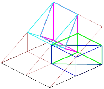
The quaquaversal tiling (Conway & Radin, 1998) is a hierarchical tiling of 3 dimensional space, based on a triangular prism that is repeatedly rotated about orthogonal axes by angles $2\pi/3$ and $\pi/2$.

The principle of our construction of the PreICs is simple. The quaquaversal tiling defines a division of space into equal volume cells. The particle distribution obtained by assigning a particle of the same mass to each cell is highly uniform: the only source of fluctuations is the redistribution of the mass at the scale of the cell. Indeed a well known argument, due to Zeldovich (Zeldovich, 1965; Zeldovich & Novikov, 1983), shows that such a local mass conservation constraint should lead to a power spectrum with the behaviour $P(k)\sim k^{2}$ at small $k$. If one adds the further constraint that the centre of mass is locally conserved one expects to obtain $P(k)\sim k^{4}$ at small $k$. Here we will impose this constraint by placing the particle in each tile at its centre of mass. Furthermore, the tiling has little preferred orientation, a desirable property which will be inherited by the particle distribution.

Consider a triangular tile, made from a 1, $\sqrt{3}$, 2 right-angle triangle, with depth 1/2. This tile can be decomposed into 4 identical tiles, all with exactly the same properties as the original “parent” tile, by placing 3 lines from the center of the long side (length 2), to the centers of the other 2 sides (length 1 and $\sqrt{3}$) and to the right angle. Then all lines are extended in depth (in the 3rd dimension). One can now choose one of two possibilities, either to rotate the two triangles at the short axis by $2\pi/3$ about an axis in the depth dimension, or to rotate the two triangles touching the right angle by $\pi/2$ about an axis in the y-dimension (see figure 1). Finally, one places two tiles next to each other, each with their choice of rotation. For further detail, see Conway & Radin (1998).

After this first tiling, we are left with 8 triangles, each identical to the original parent triangle, but a factor 8 smaller in volume. (The angles of the individual triangles are the same, only the sides are smaller by a factor 2). We can now repeat this process again for each triangle, giving us 64 identical triangles. After $N$ such iterations we will have $8^{N}$ identical triangles, with the same properties as the original parent triangle.

To obtain our configuration, we then place a particle in the center of volume of each triangle. Finally we place two parent tiles on top of each other, to form a rectangular box with sides 1,1,$\sqrt{3}$. This final distribution, which is our new PreIC to be used in simulations, thus contains $2\times 8^{N}$ particles. From now on, we will refer to this kind of particle distribution as a Q-set. For simulations where periodic boundary conditions are needed, one can only make Q-sets with $16,128,\cdots,4.2M,33.6M,\cdots$ particles. It is proved in Conway & Radin (1998) that, in the limit of an infinite number of iterations, the orientations of the tiles are essentially random (uniform in SO(3)). We infer that our distribution (with finite, but large, $N$) will have little directionality (see discussion in section 4.4).

Naturally one can imagine similar constructions based on other tilings. In this paper, however, we will focus on this simple quaquaversal structure.

3.1 COMPUTER CODE

We will briefly describe the idea behind this code. Each triangle is uniquely defined through the definition of the spatial position (in 3-d space) of 4 corners (3 corners would suffice, of course). Thus, the original parent tile is defined through 4 different $3-$vectors. This is expressed through one 12-vector, $\vec{V}$. The 8 sub-tiles in the next level of tiling, $n+1$, are defined through a constant matrix, ${\cal M}$, applied to each vector at level $n$ such that

$$\vec{V}_{i}(n+1)={\cal M}\vec{V}(n)\,,$$ (1)

where $i=1,\cdots,8$ define the 8 new sub-tiles. Thus the constant matrix ${\cal M}$ has 128 entries, and it uniquely defines each tiling step.

The code recursively applies ${\cal M}$ to the vectors (it recursively tiles each subtile), until the desired level, $N$, has been reached. Then a particle is placed in the center of volume of that triangle, and that point is written to a file. Constructed in this way the code is very fast and requires very little memory.

In our implementation the matrix ${\cal M}$ is constant. This implies that the specific rotations by fractions of $\pi$ are identical at each level of refinement. It would be possible to generalize the procedure, by allowing the rotations to differ at each level, e.g. sometimes rotate by $4\pi/3$ instead of $2\pi/3$. In that way one could achieve a slightly higher level of isotropization.

We will now consider the properties of the particle distribution in this rectangular box, in terms of mass variance and power spectrum.

4 STATISTICAL PROPERTIES

4.1 Mass Variance $\sigma_{M}^{2}(R)$

Let us first analyse the amplitude of mass fluctuations in a sphere of radius $R$ with respect to the average mass. If $M(R)$ is the mass (for a discrete distribution, the number of particles) inside a sphere of radius $R$, the normalised mass variance is defined as

$$\sigma_{M}^{2}(R)=\frac{\langle M(R)^{2}\rangle-\langle M(R)\rangle^{2}}{\langle M(R)\rangle^{2}},$$ (2)

where the brackets indicate an ensemble average. For a distribution like ours (or e.g. a grid) one can define the ensemble average as the average over random positions of the initial box. Such an ensemble average definition is equivalent to a spatial average, with the mass variance then given as the infinite volume limit of the estimator defined below.

Figure 2: The mass variance as function of radius. The correct (analytical) behaviour of the test structures are found. The Poisson (red, dotted) has $\sigma^{2}\sim R^{-3}$, the grid (black, long-dashed) has $\sigma^{2}\sim R^{-4}$ turning into $R^{-3}$ for distances much below the interparticle distance. The $\Lambda$CDM (green, dashed) has the correct behaviour until scales where the interparticle distance approaches the grid size. The Q-set (blue, solid line) has the same behaviour as a grid, namely $\sigma^{2}\sim R^{-4}$ on all scales down to the Poissonian turn over.

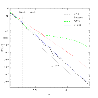
For our mass variance calculations we have used the simple estimator

$$\sigma_{M,{\rm est}}^{2}(R)=\frac{1}{\langle N_{r}\rangle^{2}}\sum_{i=1}^{N_{s}}\frac{(N_{i}(R)\ -\langle N_{r}\rangle)^{2}}{N_{s}-1}\,,$$ (3)

where $N_{i}(R)$ is the number of particles in the $i$th of $N_{s}$ randomly thrown spheres, constrained to be inside the sample volume. $\langle N_{r}\rangle$ is the mean number of particles in such a sphere, given exactly by $\langle N_{r}\rangle=\frac{4\pi r^{3}}{3v}$ where $v$ is the volume per particle (i.e. the volume of a single tile in the Q-set).

We apply this estimator to a grid, a Poisson distribution, a typical $\Lambda$CDM initial condition ($z=70$), and a Q-set. We have used $128^{3}$ particles in a cube of side unity for the first three, while the Q-set employed seven tiling levels, which gives $2\times 8^{7}=2\times 128^{3}$ particles in a rectangular box. The dimension of the Q-set box is chosen so that the mean density is equal to that of the other distributions. This is a convenient choice for comparison of the results, as it is the mean particle density $n_{0}$ which fixes the asymptotic level of the Poisson variance at small scales in any point distribution, with $\sigma_{M}^{2}(R\rightarrow 0)=\frac{1}{n_{0}V_{\rm{s}}(R)}$ where $V_{\rm{s}}=4\pi R^{3}/3$ (see e.g. Gabrielli, Joyce & Sylos Labini (2002)). Several tests confirm that our estimator calculates the correct spatial properties (see further discussion below). We see (figure 2) that the mass variance of a Q-set has the same behaviour as that of a grid with $\sigma^{2}\sim R^{-4}$ above the interparticle distance. The mean interparticle distance, $\Lambda=1/128$, for the structures with $128^{3}$ particles is also shown in the figure. Note that this is exactly the length of the shortest side of a tile in the level seven quaquaversal tiling used for the Q-set considered here.

4.2 Power Spectrum $P(k)$

The power spectrum is the primary statistical tool used to characterise fluctuations in cosmology. It is defined as

$$P({\mathbf{k}})=\lim_{V\rightarrow\infty}\frac{1}{V}\langle|\hat{\delta}(\mathbf{k})|^{2}\rangle\,,$$ (4)

where $\hat{\delta}(\mathbf{k})$ is the Fourier transform of the density fluctuation field $\delta(\mathbf{x})=(\rho(\mathbf{x})-\rho_{0})/\rho_{0}$. In the case of a discrete distribution (i.e. of point particles) these quantities simply become

$$\halign to=433.62pt{\@eqnsel\hskip\@centering$\displaystyle\let\@currentlabel=\theequation{#}$&\global\@eqcnt\@ne\hskip 2\arraycolsep\hfil${#}$\hfil&\global\@eqcnt\tw@\hskip 2\arraycolsep$\displaystyle{#}$\hfil&\llap{#}\cr 0.0pt plus 1000.0pt$\displaystyle{ \delta(\mathbf{x}) &10.0pt\hfil${=&10.0pt$\displaystyle{\frac{V}{N_{\rm{p}}} \sum\delta_{\rm{D}}(\mathbf{x}-\mathbf{x}_{\rm p}) -1 \, , {}&\hbox to0.0pt{\hss{\rm(5-a)}\cr\penalty 100\vskip 3.0pt\vskip 0.0pt\cr 0.0pt plus 1000.0pt$\displaystyle{\hat{\delta}(\mathbf{k}) &10.0pt\hfil${=&10.0pt$\displaystyle{\frac{V}{N_{\rm{p}}} \sum e^{-i \mathbf{k}\cdot\mathbf{x}_{\rm p}} \qquad(\mathbf{k}\neq 0) \, , &\hbox to0.0pt{\hss{\rm(5-b)}\cr}}}}}}}}}$$

where $\mathbf{x}_{\rm p}$ is the location of each particle and $\delta_{\rm{D}}$ is the Dirac delta function.

To estimate the power spectrum we have used the “brute force” method i.e. we calculate it directly from the formula one obtains by substituting Eq. (4.2) in Eq. (4), without the infinite volume limit and ensemble average. Our finite volume $V$ is thus a rectangular box with sides $L_{i}$, and we assume periodic boundary conditions so that $\mathbf{k}$ in the Fourier sums take the values $\mathbf{k}=2\pi\left(n_{x}/L_{x},n_{y}/L_{y},n_{z}/L_{z}\right)$ where $n_{i}$ are integers. We obtain $P(k)=P(|\mathbf{k}|)$ by averaging over a bin of finite width around $k=|\mathbf{k}|$ (Sirko, 2005). It is important to take care in the interpretation of the large scale (i.e. small $k$) modes, which will be affected both by under-sampling and contaminated by the boundary conditions (which systematically suppress power at small $k$). With this simple estimator, however, we do not have to worry about the effect of assignment function, which typically causes problems in FFT methods (Jing, 2005).

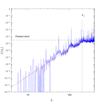
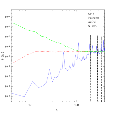
As for the mass variance we calculate the power spectrum for a grid, a Poisson distribution, a typical $\Lambda$CDM initial condition, and a Q-set. This time we use a smaller number of particles in order to facilitate the more computationally demanding procedure of calculating $P(k)$: they all have $32^{3}$ particles except for the Q-set which has $N=5$, and therefore again has twice as many points ($32^{3}=8^{5}$). Likewise for the mass variance, this makes the the Poisson level ($V/N_{\rm{p}}$) the same for all the distributions considered.

We see in figure 3 that the Q-set has the anticipated $P(k)\sim k^{4}$ behaviour up to the wave vector for the mean interparticle separation, $k_{\Lambda}=2\pi/\Lambda$, where it flattens on average, to the Poisson level. We have used a very fine binning in order to capture this characteristic slope as well as the peaks arising from typical interparticle distances. We note that peaks appear at frequencies of $2^{-n}k$, where $n$ has integer values. It can be shown (see  Radin (1999)) that in hierarchical structures, a feature in real space between two radii, $r_{1}$ and $r_{2}$, also must appear between the radii $\kappa r_{1}$ and $\kappa r_{2}$, where $\kappa=2$ for a quaquaversal structure.

Consistent with this interpretation we note that adding random perturbations to the particles, hence creating a shuffled Q-set, gives $P(k)\sim k^{2}$ with peaks of diminished amplitude.

A comparison between the different distributions can be seen in figure 4. Note that the grid has zero power up $k_{\Lambda}$ where it is strongly peaked and that all distributions, on average, reach the Poisson level at this wave number.

Figure 3: Detailed plot of the power spectrum for a the Q-set. We have used a very fine binning to capture the $k^{4}$ slope as well as the characteristic peaks of this PreIC.

Figure 4: The power spectra for a Q-set (solid, blue), a grid (short-dashed, black), a Poisson distribution (dotted, red) and a $\Lambda$CDM initial condition (long-dashed, green) . The Q-set shows a $k^{4}$ behaviour up to the Poisson level. The power spectrums has characteristic peaks appearing, as discussed in the text, at $k/2,k/4,k/8\ldots\,$ due to the hierarchical properties of the Q-set.

4.3 Relations between $\sigma_{M}^{2}(R)$ and $P(k)$

$\sigma^{2}(R)$ and $P(k)$ are related by the standard expression

$$\sigma_{M}^{2}(R)=\frac{1}{2\pi^{2}}\int_{0}^{+\infty}P(k)\hat{W}^{2}(kr)k^{2}dk\,,$$ (6)

where $\hat{W}^{2}(kr)$ is the Fourier transform of the spherical top hat window function.

By studying Eq. (6) for a power spectrum of the form $P(k\rightarrow 0)\sim k^{n}$ one finds  (Gabrielli, Joyce & Sylos Labini, 2002) that for $R\rightarrow\infty$

$$\sigma_{M}^{2}(R)\sim\left\{\begin{array}[]{lll}1/R^{3+n}\;\;\mbox{if}\;\;n<1\\ \log(R)/R^{4}\;\;\mbox{if}\;\;{n=1}\\ 1/R^{4}\;\;\mbox{if}\;\;{n>1}\end{array}\right.$$ (7)

Two particular and simple examples which are useful reference points against which to gauge new distributions are:

• Poisson: $\sigma_{M}^{2}(R)\sim R^{-3}$, $P(k)\sim V/N_{\rm p}\sim const$

• Shuffled Lattice: $\sigma_{M}^{2}(R)\sim R^{-4}$, $P(k)\sim k^{2}$

The numerical results for the mass variance and power spectrum in the previous two sections are all in line with these analytic results, notably our new Q-set has $\sigma_{M}^{2}(R)\sim R^{-4}$ and $P(k)\sim k^{4}$. This (large scale) behaviour makes the Q-set a member of a group of systems which have been termed super-homogenous  (Gabrielli, Joyce & Sylos Labini, 2002; Gabrielli et al., 2003) or hyperuniform  (Torquato & Stillinger, 2003). Such distributions, defined by the property $P(k\rightarrow 0)=0$, are characterised in real space (cf. Eq. (7) above) by the asymptotic behaviour of their variance, $\sigma^{2}(R)\sim 1/R^{m}$ with $d<m<d+1$ where $d$ is the spatial dimension. This quantity thus decays faster than in a Poisson point process ($m=d$), and in the cases we have considered attains the behaviour ($m=d+1$). This is in fact the fastest possible decay of this quantity for either point (Beck, 1987) or continuous (Gabrielli, Joyce & Sylos Labini, 2002) mass distributions. We note that the glass PreIC also belong to this class, as it shares this same behaviour of the variance and power spectrum as the Q-set we have introduced and analysed.

Figure 5: $\theta$ and $\phi$ are the standard angles in spherical coordinates, giving the orientations of a chosen reference vector in each tile of a level 7 Q-set (blue triangles), and the analagous quantities for a grid (red open circles).

4.4 Isotropy

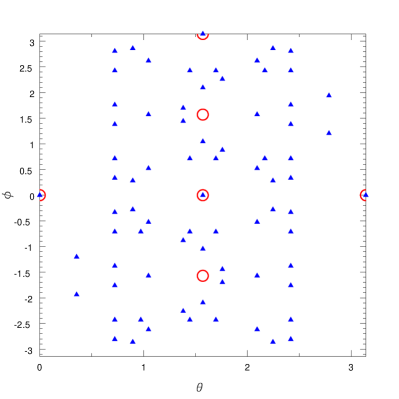
One of the nice features of the Q-set is, as we have underlined, that it is isotropic. This result applies, however, in the limit of an infinite number of iterations of the algorithm we have described. It it interesting to quantify the degree of isotropy of a finite level tiling. To do so we show in Figure 5 a plot giving (blue triangles) the distinct directions defined by the tiles of the quaquaversal tiling used to construct the Q-set with $N=7$. The directions are those of the shortest axis of each tile with respect to the orientation of the mother tile. Also shown (red open circles) is an analagous characterisation of a grid, which gives just the six orientations of the vectors pointing to nearest neighbour sites.

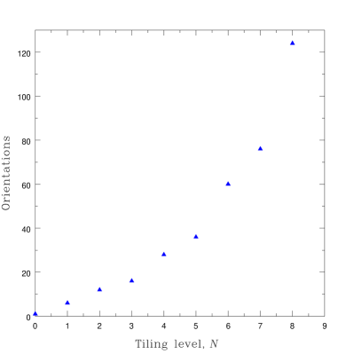
Figure 6 shows, on the other hand, the dependence of the number of distinct orientations, in the $(\theta,\phi)$-plane, on the level of the tiling. The degree of isotropy grows very rapidly with increasing $N$.

Figure 6: Number of distinct orientations as a function of level of tiling.

5 CONCLUSIONS

We have studied an alternative to the standard pre-initial conditions for N-body simulations of cosmological structures. The standard grid has strong orientations, and the glass is poorly defined and computationally expensive to create. We have therefore considered a particle distribution created starting from an equal volume tiling of space, called the quaquaversal tiling. The particle distribution is trivial to create, has virtually no orientation (is statistically isotropic), and has rapidly vanishing large scale power-spectrum. We provide a C-code for the generation of these structures on http://krone.physik.unizh.ch/~hansen/qua/.

References

- Beck (1987) Beck, J. 1987, Acta Mathematica 159, 1-878282
- Bode et al. (2001) Bode, P., Ostriker, J. P., & Turok, N. 2001, ApJ, 556, 93
- Carr (1961) Carr, H. 1961, Phys. Rev. 122, 1437
- Conway & Radin (1998) Conway, J. H. & Radin, C. 1998, Inventiones math. 132, 179
- Efstathiou et al. (1985) Efstathiou, G., Davis, M. Frenk, C. S. & White, S. D. M. 1985, Astrophys. J. Suppl. 57, 241
- Götz & Sommer-Larsen (2003) Götz, M., & Sommer-Larsen, J. 2003, Ap&SS, 284, 341
- Gabrielli, Joyce & Sylos Labini (2002) Gabrielli, A. Joyce, M. & Sylos Labini, F. 2002, Phys. Rev. D65, 083523
- Gabrielli et al. (2003) Gabrielli, A., Jancovici, B., Joyce, M., Lebowitz, J.L., Pietronero, L. & Sylos Labini, F. 2003, Phys.Rev. D67, 043506.
- Jing (2005) Jing, Y. P. 2005, Astrophys. J. 620, 559
- Joyce et al. (2005) Joyce, M., Marcos, B., Gabrielli, A., Baertschiger, T. & Sylos Labini, F. 2005, Phys. Rev. Lett. 95, 011304
- Melott et al. (1997) Melott A., Shandarin S., Splinter R. & Suto, Y. 1997, Astrophys. J. Lett., 479, L79
- Radin (1999) Radin C. 1999, J. Stat. Phys. 95, 827
- Smith et al. (2003) Smith, R. et al. 2003, MNRAS 341, 1311
- Sirko (2005) Sirko, E. 2005, “Initial conditions to cosmological N-body simulations, or how to run an ensemble of simulations,” Astrophys. J. 634, 728 [arXiv:astro-ph/0503106].
- Torquato & Stillinger (2003) Torquato, S. & Stillinger, F.H. 2003, Phys. Rev. E68, 041113
- White (1994) White, S. D. M. 1994, arXiv:astro-ph/9410043
- Zeldovich (1965) Zeldovich, Ya. B., Adv. Aston. Ap., 3, 241
- Zeldovich & Novikov (1983) Zeldovich, Ya. B. & Novikov, I.D. 1983,, Relativistic Astrophysics. Part 2. The structure and evolution of the Universe, The University of Chicago Press, Chicago and London