Observational constraints on phantom-like braneworld cosmologies

Abstract

We investigate a simple braneworld model in which the universe contains only cold dark matter and a cosmological constant, but the effective dark energy is phantom-like because of extra-dimensional gravity effects. Modified gravity screens the cosmological constant $\Lambda$, allowing for a larger $\Lambda$. In practice, observations do not favour any significant screening. We use supernova data, the cosmic microwave background shift parameter, and the baryon oscillation peak in the galaxy distribution to constrain the model. We find the mean value of $\Omega_{\text{m}}$ with 68% confidence limits, and an upper limit on $\Omega_{\Lambda}$ at the 68% confidence level. The best-fit model is very close to a standard LCDM model, but the LCDM model provides a better fit since it has one less parameter.

I Introduction

There is increasingly strong evidence for the acceleration of the late-time universe, from observations of supernovae, cosmic microwave background anisotropies and the large-scale structure. This late-time acceleration poses a major theoretical challenge in cosmology Padmanabhan:2006ag . Within the framework of general relativity, the acceleration originates from a dark energy field with effectively negative pressure: $w\equiv p/\rho<-{1\over 3}$. (It is also conceivable, though it remains controversial, that acceleration may be due to nonlinear backreaction or averaging effects Kolb:2005me .) The simplest model, with cosmological constant or vacuum energy ($w=-1$) as dark energy, i.e., the LCDM model, provides a very good fit to the data Spergel:2006hy , but the unnaturally small and fine-tuned value of $\Lambda$ cannot be explained within current particle physics. Quintessence models, i.e. scalar fields with $w>-1$, allow for richer dynamical behaviour, but do not improve the fit to the data, and also do not lessen the severe theoretical problems faced by LCDM. “Phantom” models, with $w<-1$, violate the null energy condition $\rho+p\geq 0$, and as a result, the total phantom energy density grows with expansion. Phantom scalar fields share the theoretical problems of quintessence, but in addition, they have negative kinetic energy and lead to an unstable quantum vacuum Carroll:2003st .

Current observations are compatible with $w<-1$. The WMAP 3-year data, in combination with large-scale structure and SN data, allows for $w<-1$ in a general relativistic model: for constant $w$ Spergel:2006hy ,

$$w=-1.06^{+.13}_{-.08}\,.$$ (1)

The simplest way to produce $w<-1$ is a phantom scalar field in general relativity. But the price is instability. Thus it is interesting to investigate other models in which $w<-1$, but without negative kinetic energy or associated instabilities. This can happen if some other effect mimics phantom dynamics, i.e., leads to an effective $w_{\text{eff}}$ such that $w_{\text{eff}}<-1$, but without the presence of a pathological phantom field.

For example, Boisseau et al. Boisseau:2000pr showed that this can happen in scalar-tensor theories. A number of other possible mechanisms for mimicking phantom behaviour has recently been investigated Liu:2003dj , including nonminimal coupling to gravity, interactions between dark energy and the matter sector, modified Lagrangians, braneworld models and quantum effects. Many of these mechanisms require complicated additional features and fine-tunings – it is not easy to construct simple and natural phantom-like behaviour without a phantom field. Among the less complicated models is that of Csaki et al. Csaki:2004ha , in which photon-to-axion conversion mimics super-acceleration (in the presence of non-phantom dark energy).

Phantom behaviour may also occur in braneworld models with an infrared modification of general relativity, as pointed out by Sahni and Shtanov Sahni:2002dx . A special case of the Sahni-Shtanov models was further investigated by Lue and Starkman Lue:2004za . In these models, the 4-dimensional brane universe contains only matter and a cosmological constant $\Lambda$, but a 5-dimensional gravitational effect leads to phantom behaviour. The most important implication of this modified gravity effect is that $\Lambda$ is effectively screened, so that in principle a higher value of $\Lambda$ is allowed by the observations than in the LCDM case. These models are the simplest in the Shani-Shtanov class, with only one parameter more than the LCDM model, and they are the simplest braneworld models with phantom behaviour as far as we are aware. In this paper, we extend the investigation of Lue and Starkman by testing the models against observations, to see how the data constrains the model parameters, and to compare the goodness of fit to that of LCDM. As explained below, this test can only be partially carried out, since the CMB anisotropies and matter power spectrum for the model have not yet been computed, and this remains a formidable open problem. However we can apply geometric observational tests that are based on the background dynamics.

II The phantom-like braneworld

The Dvali-Gabadadze-Porrati (DGP) braneworld model, generalized to cosmology by Deffayet Dvali:2000rv , is a self-accelerating model without any form of dark energy. In fact, the self-accelerating models are not the only form of DGP model. There are two separate branches, DGP$(\pm)$, depending on how the 4D brane universe is embedded in the 5D spacetime.

• The (+) branch is the self-accelerating model, which has recently been tested against supernova (SN) and baryon oscillation (BO) observations Fairbairn:2005ue , and then in addition against the CMB shift data Maartens:2006yt . The flat DGP(+) model is outside the 2$\sigma$ contour for the joint SN and BO constraints, but this is somewhat misleading, since the CMB observations have not been applied. When the CMB shift constraint is included, the flat DGP(+) model is within the 2$\sigma$ contour for the joint constraints, but the best-fit LCDM model gives a significantly better fit to the data Maartens:2006yt .

• The DGP$(-)$ model is very different. It does not self-accelerate, but requires dark energy on the brane. The simplest model has a cosmological constant, and we will call this the LDGP model, following Ref. Lue:2004za . The LDGP model is a special case of the Sahni-Shtanov models with zero brane tension. It experiences 5D gravitational modifications to its dynamics, which effectively screen the cosmological constant. At late times, as gravity leaks off the 4D brane, the dynamics deviates from general relativity. The transition from 4D to 5D behaviour is governed by a crossover scale $r_{c}$, as in the (+) branch. (The LDGP model has recently been generalized by replacing the cosmological constant with a quintessence field Chimento:2006ac .)

The energy conservation equation for LDGP remains the same as in general relativity, but the Friedman equation is modified:

$$\dot{\rho}+3H(\rho+p)=0\,,$$ (2)

$$H^{2}+{H\over r_{c}}={8\pi G\over 3}\rho+{\Lambda\over 3}\,.$$ (3)

[The self-accelerating (+) branch has $-H/r_{c}$ instead of $+H/r_{c}$.] For the CDM case, with $p=0$, these equations imply

$$\dot{H}=-4\pi G\rho\left[1-{1\over\sqrt{1+32\pi Gr_{c}^{2}\rho/3+4r_{c}^{2}\Lambda/3}}\right].$$ (4)

Equation (3) shows that at early times, the general relativistic Friedman equation is recovered:

$$H\gg r_{c}^{-1}~{}\Rightarrow~{}H^{2}\approx{8\pi G\over 3}\rho+{\Lambda\over 3}\,.$$ (5)

By contrast, at late times, the $H/r_{c}$ term is important and the Friedman equation is nonstandard.

Figure 1: (a) and (b): $1+w_{\text{eff}}$ against $1+z$. (c): $1+w_{\text{tot}}$ against $1+z$, with the same parameters as (a).
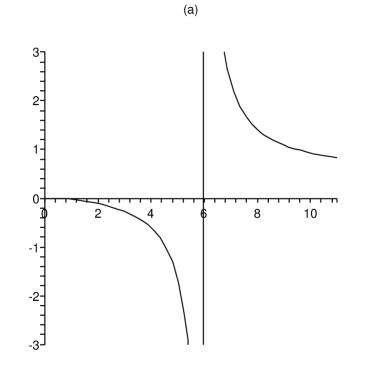
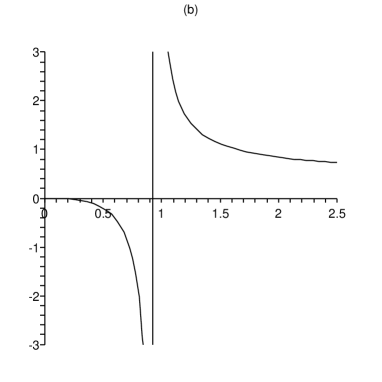
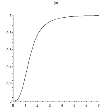
(a) shows a typical model with $w_{\text{eff}}<-1$ at $z=0$, with parameters $(\Omega_{\text{m}},\Omega_{\Lambda})=(0.3,0.8)$. (b) shows a model with unrealistic parameters, $(\Omega_{\text{m}},\Omega_{\Lambda})=(1.1,1.4)$, that has $w_{\text{eff}}>-1$ at $z=0$. Note that $w_{\text{eff}}\to-1$ as $z\to-1$ ($a\to\infty$), and $w_{\text{eff}}\to-{1\over 2}$ as $z\to\infty$. The redshift $z_{*}$ where $w_{\text{eff}}$ goes through $\pm\infty$ is clearly evident, with $z_{*}>0$ in (a) and $z_{*}<0$ in (b). Note that $w_{\text{tot}}$ is continuous at $z_{*}$.

Gravity leakage at late times screens the cosmological constant, leading to an effective dark energy Sahni:2002dx ; Lue:2004za

$$\rho_{\text{eff}}={1\over 8\pi G}\left(\Lambda-3{H\over r_{c}}\right),$$ (6)

where

$$H^{2}={8\pi G\over 3}(\rho+\rho_{\text{eff}}).$$ (7)

By Eq. (4), $\dot{H}<0$, so that

$$\dot{\rho}_{\text{eff}}>0\,.$$ (8)

This is the basis for the phantom-like behaviour in the model. We can define the effective dark energy equation of state $w_{\text{eff}}=p_{\text{eff}}/\rho_{\text{eff}}$ via

$$\dot{\rho}_{\text{eff}}+3H(1+w_{\text{eff}})\rho_{\text{eff}}=0\,,$$ (9)

or equivalently,

$$\dot{H}=-4\pi G[\rho+(1+w_{\text{eff}})\rho_{\text{eff}}].$$ (10)

Thus $\rho_{\text{eff}}$ and $w_{\text{eff}}$, as defined in Eqs. (6)–(10), are effective quantities that give a standard general relativistic interpretation of LDGP expansion history, i.e., they describe the equivalent general relativity model. This equivalent model is a phantom model: by Eqs. (6) and (9), we have

$$1+w_{\text{eff}}={\dot{H}\over 8\pi Gr_{c}H\rho_{\text{eff}}}\,.$$ (11)

Since $\dot{H}<0$ by Eq. (10), we have effective phantom behaviour,

$$w_{\text{eff}}<-1~{}~{}~{}(\rho_{\text{eff}}>0)\,.$$ (12)

The effective picture breaks down when $\rho_{\text{eff}}=0$, i.e., when $H=H_{*}=r_{c}\Lambda/3$, which always happens at some redshift $z_{*}$ in the history of the universe. At this time, $w_{\text{eff}}\to-\infty$. At higher redshifts, $1+w_{\text{eff}}$ is positive, decreasing from $+\infty$, as illustrated in Fig. 1. This is a special case of the behaviour found by Sahni and Shtanov Sahni:2002dx . Nothing unphysical occurs at $z_{*}$, it is only the description that breaks down. Note that it is possible that $z_{*}<0$, i.e., in the future, so that $H_{0}>H_{*}$. But in this case, $w_{\text{eff}}$ at $z=0$ is positive, so that there is no phantom behaviour for nonnegative redshifts. In fact, Eq. (22) below shows that this only occurs for the unphysical parameter values, $\Omega_{\text{m}}>1$.

Although $w_{\text{eff}}\to-{1\over 2}$ for large redshifts, CDM is becoming strongly dominant, so that the geometrical constraints from observations can be comfortably satisfied – as we show in the next section. As discussed further in the concluding section, it remains an open question whether structure formation constraints can also be satisfied.

The effective phantom behaviour in LDGP has no associated instability, unlike phantom scalar fields in general relativity. Furthermore, in general relativistic phantom models, $\dot{H}$ eventually becomes positive, i.e., the universe eventually super-accelerates, which can lead to a “big rip” singularity Nojiri:2005sx . This also happens in a number of models that mimic phantom behaviour without phantom matter. By contrast, in LDGP, $\dot{H}$ is always negative, and there is no big rip singularity in LDGP. Equation (10) shows that the key issue is the sign of $1+w_{\text{eff}}$ as $a\to\infty$. In phantom and most phantom-like models, $1+w_{\text{eff}}<0$ as $a\to\infty$, so that $\dot{H}$ becomes positive. In LDGP, we have $1+w_{\text{eff}}\to 0^{-}$ and the universe is asymptotically de Sitter:

$$w_{\text{eff}}\to-1\,,~{}H\to H_{\text{dS}}={1\over 2r_{c}}\left[\sqrt{{4r_{c}^{2}\Lambda\over 3}+1}-1\right].$$ (13)

Note that $H_{\text{dS}}$ is less than the corresponding LCDM value $H_{\text{dS,LCDM}}=\sqrt{\Lambda/3}$. This is an aspect of the effective screening of $\Lambda$ by DGP($-$) gravity.

In LDGP, the total equation of state parameter is always greater than $-1$, i.e., the phantom effects never dominate. Although the screened dark energy has phantom equation of state, $w_{\text{eff}}<-1$, the total $w$ remains above $-1$, and there is no phantom-like acceleration of the universe, and thus no big rip. This is shown by Eq. (23) below, and illustrated in Fig. 1.

III Observational constraints on LDGP

Figure 2: The 68%, 95% and 99% confidence contours for the SNLS data (left), the CMB shift parameter $S$ (based on WMAP 3-year data) (middle) and the baryon oscillation measure $A$ (right). The shaded area is the unphysical region, $\Omega_{\text{m}}+\Omega_{\Lambda}<1$, and the boundary is the flat LCDM model, $\Omega_{r_{c}}=0$.

In dimensionless form, the LDGP Friedman equation (3) implies

$$E(z)\!\equiv\!{H(z)\over H_{0}}=\!\sqrt{\Omega_{\text{m}}(1+z)^{3}+\Omega_{\Lambda}+\Omega_{r_{c}}}-\!\sqrt{\Omega_{r_{c}}},$$ (14)

where

$$\Omega_{\text{m}} = {8\pi G\rho_{0}\over 3H_{0}^{2}}\,,~{}\Omega_{\Lambda}={\Lambda\over 3H_{0}^{2}}\,,$$ (15)

$$\Omega_{r_{c}} = {1\over 4H_{0}^{2}r_{c}^{2}}\,.$$ (16)

Note that Eq. (3) implies

$$\Omega_{\text{m}}+\Omega_{\Lambda}=1+2\sqrt{\Omega_{r_{c}}}\,,$$ (17)

so that in particular,

$$\Omega_{\text{m}}+\Omega_{\Lambda}\geq 1\,.$$ (18)

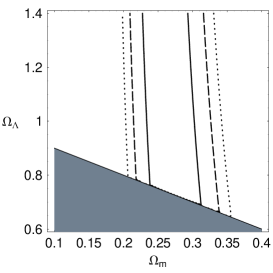
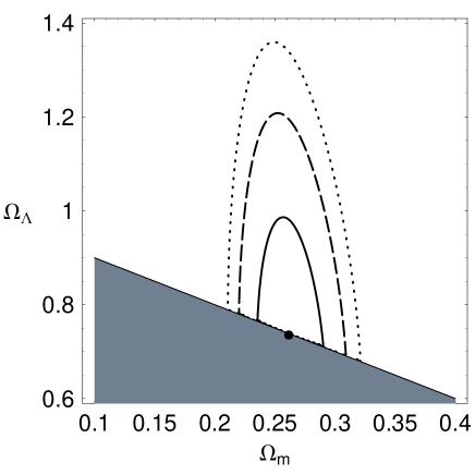
This condition ensures that $H_{0}^{2}\geq 0$. The flat LCDM model is the limiting case of equality, when $\Omega_{r_{c}}=0$. The unphysical region $\Omega_{\text{m}}+\Omega_{\Lambda}<1$ (corresponding to imaginary $H_{0}$) is shown in Fig. 2.

Equation (17) means that the flat LDGP model has the remarkable feature that it mimics a closed LCDM model in the $(\Omega_{\text{m}},\Omega_{\Lambda})$ plane:

$$\sqrt{\Omega_{r_{c}}}\leftrightarrow-{\Omega_{K}\over 2}\,.$$ (19)

The WMAP 3-year data with SN data gives Spergel:2006hy

$$\Omega_{K}=-0.01^{+.016}_{-.009}\,,~{}~{}\Omega_{\Lambda}=0.72\pm.04\,.$$ (20)

If we take the mean value, $\Omega_{K}=-0.01$, then Eq. (19) gives the “equivalent” value $r_{c}=100H_{0}^{-1}$. This very large value of $r_{c}$ suggests that observations will require the LDGP model to be close to the LCDM model ($r_{c}=\infty$). We confirm this expectation below.

By Eqs. (11) and (14), we have

$$1+w_{\text{eff}}(z)=-{\sqrt{\Omega_{r_{c}}}\Omega_{\text{m}}(1+z)^{3}\over[\Omega_{\Lambda}-2\sqrt{\Omega_{r_{c}}}\,E(z)][\sqrt{\Omega_{r_{c}}}+E(z)]}\!.$$ (21)

This equation shows explicitly how we can mimic the expansion history of LDGP by an effective phantom model in general relativity. However, there is no violation of the null energy condition, and no super-acceleration, since in LDGP the phantom dynamics is gravitational. Figure 1 illustrates this equation.

At the current time,

$$1+w_{\text{eff}}(0)=-{(\Omega_{\text{m}}+\Omega_{\Lambda}-1)\Omega_{\text{m}}\over(1-\Omega_{\text{m}})(\Omega_{\text{m}}+\Omega_{\Lambda}+1)}.$$ (22)

Provided that $\Omega_{\text{m}}<1$, we have phantom behaviour at the current time, i.e., Eq. (12) is satisfied.

As noted above, the phantom effects never dominate, and the total equation of state parameter, $w_{\text{tot}}=p_{\text{tot}}/\rho_{\text{tot}}=w_{\text{eff}}\rho_{\text{eff}}/(\rho+\rho_{\text{eff}})$, is always greater than $-1$. By Eqs. (14) and (21),

$$1+w_{\text{tot}}(z)={\Omega_{\text{m}}(1+z)^{3}\over E(z)\left[\sqrt{\Omega_{r_{c}}}+E(z)\right]}\,,$$ (23)

and it follows immediately that $w_{\text{tot}}(z)\geq-1$. Since $E\to\sqrt{\Omega_{\Lambda}+\Omega_{r_{c}}}-\sqrt{\Omega_{r_{c}}}$ as $z\to-1$ (i.e., as $a\to\infty$), it follows that $1+w_{\text{tot}}\to 0^{+}$. At early times, i.e., $z\to\infty$, we have $w_{\text{tot}}\to 0$, which is the GR limit (we are neglecting radiation). This behaviour is illustrated in Fig. 1.

From Eq. (4), the dimensionless acceleration is

$${\ddot{a}/a\over H_{0}^{2}}=E\!\left[\!{2\Omega_{r_{c}}+2\Omega_{\Lambda}-\Omega_{\text{m}}(1+z)^{3}\over 2\sqrt{\Omega_{\text{m}}(1+z)^{3}+\Omega_{\Lambda}+\Omega_{r_{c}}}}\!-\!\sqrt{\Omega_{r_{c}}}\right],$$ (24)

so that the redshift when acceleration starts is given by

$$\!\!\!\!\!\!\!1+z_{\text{acc}}=$$

$$\!\!\!\!\left(2{\Omega_{\Lambda}\over\Omega_{\text{m}}}\right)^{\!1/3}\left[\!1+2{\Omega_{r_{c}}\over\Omega_{\Lambda}}\!\left(\!1-\!\sqrt{1+{3\Omega_{\Lambda}\over 4\Omega_{r_{c}}}}\,\right)\right]^{\!1/3}\!.$$ (25)

The LCDM result is recovered for $\Omega_{r_{c}}=0$. When $z_{\text{acc}}=0$, this gives the critical line $\Omega_{\Lambda}=2\Omega_{\text{m}}-1$, so that

$$\Omega_{\text{m}}<{1\over 2}(1+\Omega_{\Lambda})\,,$$ (26)

is the condition for models that are currently accelerating. This differs from the corresponding condition for LCDM, i.e., $\Omega_{\text{m}}<2\Omega_{\Lambda}$.

The fundamental test of the background dynamics of a cosmological model is the SN magnitude-redshift test, based on the luminosity distance,

$$d_{L} = {(1+z)\over H_{0}}\,\int_{0}^{z}\,{dz^{\prime}\over E(z^{\prime})}\,.$$ (27)

(Here we are restricting to the flat case.) The 68%, 95% and 99% confidence contours from fits to the Legacy (SNLS) data Astier:2005qq are shown in the LDGP parameter plane in Fig. 2.

Further independent tests are needed to check whether the LDGP model is consistent with the observed features of the universe.

Figure 3: Joint constraints on LDGP models from the SNLS data, the BO measure $A$ and the CMB shift parameter $S$. The solid dot is the best-fit model. The shaded area is the unphysical region, $\Omega_{\text{m}}+\Omega_{\Lambda}<1$, and the boundary is the flat LCDM model, $\Omega_{r_{c}}=0$.

The CMB shift parameter

$$S=\sqrt{\Omega_{\text{m}}}H_{0}\,{d_{L}(z_{\text{r}})\over(1+z_{\text{r}})}\,,$$ (28)

encodes the relation between the angular diameter distance to last scattering, the angular scale of the first acoustic peak, and the physical scale of the sound horizon. This parameter is effectively model-independent and provides a good test of the background dynamics, independent of the SN redshift test. We take $z_{\text{r}}=1090$. Wang and Mukherjee Wang:2006ts have used the WMAP 3-year data to find that

$$S=1.70~{}\pm 0.03\,.$$ (29)

This value shows a significant improvement in the error over the value from the 1-year data Wang:2003gz , $S=1.72\pm 0.06$. The constraints from the CMB $S$ parameter, based on the 3-year data, are shown in Fig. 2.

Figure 4: The normalized marginalized likelihoods for $\Omega_{\text{m}}$ and $\Omega_{\Lambda}$, subject to the joint constraints of data from SNLS supernova redshifts, CMB shift parameter $S$, and baryon acoustic oscillation measure $A$.

The baryon acoustic oscillation peak recently detected in the SDSS luminous red galaxies (LRGs) Eisenstein:2005su can be used as another independent geometrical test of the LDGP. The correlation function for SDSS LRGs shows a peak at a scale $\sim 100h^{-1}\,$Mpc, corresponding to the first acoustic peak at recombination (determined by the sound horizon). The observed scale effectively constrains the quantity Eisenstein:2005su

$$A = \sqrt{\Omega_{\text{m}}}\left[{H_{0}^{3}\,d_{L}^{2}(z_{1})\over H_{1}z_{1}^{2}(1+z_{1})^{2}}\right]^{1/3},$$ (30)

where $z_{1}=0.35$ is the typical LRG redshift. Eisenstein et al. Eisenstein:2005su give

$$A=0.469\pm 0.017\,.$$ (31)

(We have suppressed a weak dependence of $A$ on the spectral tilt.) Note that there is a level of uncertainty in the use of the BO measure $A$ to test non-LCDM models. This uncertainty will require substantial further effort, both in the processing of the data Maartens:2006yt ; Dick:2006ev and in the theoretical understanding of the LDGP matter power spectrum (see Ref. Maartens:2006yt and the discussion below). For the present, we use the constraint in Eq. (31), and assume that the unresolved issues will lead to only small corrections. Constraints from the BO data are shown in Fig. 2.

The joint constraints from SN, CMB shift and BO data are shown in Fig. 3.

IV CONCLUSIONS

A naive comparison between LDGP models and closed LCDM models, as illustrated in Eqs. (19) and (20), already suggests that the data will favour LDGP models that are close to the flat LCDM model. The joint constraint contours in Fig. 3 confirm this expectation.

The best fit from the joint constraints is

$$\Omega_{\text{m}}=0.26\,,~{}\Omega_{\Lambda}=0.74\,,~{}w_{\text{eff}}(0)=-1.00\,,$$ (32)

with $\chi^{2}$ of

$$\chi^{2}=114.6\,,~{}~{}\chi^{2}~{}\text{per degree of freedom}\,=0.996\,.$$ (33)

Interestingly, the best-fit LDGP model, with current data and within the accuracy of our calculations, is the LCDM limit of LDGP. Since the LCDM model has one less parameter, it provides a better fit as measured by the reduced $\chi^{2}$:

$$\chi^{2}\Big{|}_{\text{LCDM}}~{}\text{per degree of freedom}\,=0.988\,.$$ (34)

It is the CMB shift value from the 3-year WMAP data that is forcing the best-fit strongly towards the LCDM limit: if we use the shift value from the 1-year data Wang:2003gz , i.e., $S=1.72\pm 0.06$, then the best-fit model from the joint constraints moves off the LCDM boundary:

$$\Omega_{\text{m}}=0.27\,,~{}\Omega_{\Lambda}=0.78\,,~{}w_{\text{eff}}(0)=-1.01~{}(\text{1-year }\,S)\,,$$ (35)

with $\chi^{2}=113.7$, and a reduced $\chi^{2}$ per degree of freedom of $0.988$.

The best-fit LDGP model happens to be an LCDM model, using the current data, but it is more meaningful to give the 68% confidence limits on the mean values of the parameters. The 68% contour in Fig. 3 shows that a broad range of non-LCDM models is consistent with the joint data constraints. In principle, we can calculate this range by marginalizing in turn over $\Omega_{\Lambda}$ and $\Omega_{\text{m}}$. In practice this is made difficult by the asymmetrical shape of the physical region in parameter space. The marginalized likelihoods are shown in Fig. 4. The $\Omega_{\text{m}}$ likelihood has a near-gaussian shape, so that the median gives a good measure of the mean. Then we can calculate the limits by integrating to 34.1% of the area to the left and 34.1% to the right. This leads to

$$\Omega_{\text{m}}=0.261^{+0.019}_{-0.018}\,.$$ (36)

By contrast, the $\Omega_{\Lambda}$ likelihood curve is strongly asymmetrical, reflecting the fact that the unphysical region has a stronger effect on $\Omega_{\Lambda}$ than on $\Omega_{\text{m}}$. As a consequence, the mode and the median are significantly different, and we cannot extract a meaningful mean value for $\Omega_{\Lambda}$. A conservative upper limit on $\Omega_{\Lambda}$ may be computed by integrating from the mode until 68% of the area under the curve. This gives

$$\Omega_{\Lambda}<0.95~{}\text{ at 68.3\% confidence}\,.$$ (37)

If we use the Gold SN data Riess:2004nr instead of the SNLS data, then there are some interesting changes in the values of the parameters, but the best fit lies still on the LCDM line. The Gold data favours a higher best-fit $\Omega_{\text{m}}$:

$$\Omega_{\text{m}}=0.275\,,~{}\Omega_{\Lambda}=0.725\,,$$ (38)

$$\chi^{2}=179.3\,,~{}\chi^{2}~{}\text{per degree of freedom}\,=1.142\,.$$ (39)

For LCDM the $\chi^{2}$ per degree of freedom is 1.135. The marginalized likelihoods for $\Omega_{\text{m}}$ and $\Omega_{\Lambda}$ are shown in Fig. 5. We find that

$$\Omega_{\text{m}}=0.274^{+0.019}_{-0.019}\,,$$ (40)

$$\Omega_{\Lambda}<0.87~{}\text{ at 68.3\% confidence}\,.$$ (41)

Thus the Gold data gives a stronger upper limit on $\Omega_{\Lambda}$.

Figure 5: As in Fig. 4, but using the Gold supernova data.

Equations (36), (37) and (40), (41) summarize our quantitative conclusions about the observational constraints on LDGP models. The 3 independent data sets allow for a significant range of these phantom-like braneworld models, with $\Omega_{\text{m}}$ values that are consistent with other observational tests, and with $\Omega_{\Lambda}$ values that imply significant screening of $\Lambda$. However, the LCDM model, with one less parameter, does provide a better fit to the data. The evidence for braneworld screening of $\Lambda$, via effective phantom behaviour, is therefore weak. This is consistent with results for general relativistic models. If one uses only supernova observations, especially the Gold data Riess:2004nr , then there appears to be evidence for phantom dark energy. But it is misleading to ignore the CMB observations, and when these are imposed, the evidence for phantom behaviour is much weaker Jassal:2006gf .

It is important to stress that we have only imposed observational tests on the background dynamics of LDGP. In regard to background dynamics, which are determined by $H(z)$, the LDGP model is indistinguishable from a GR model with dark energy whose equation of state is exactly $w_{\text{eff}}(z)$, as given by Eq. (21). However, the GR model has no physical motivation, whereas the LDGP model gives a covariant and consistent physical meaning to the equation of state (21). Nevertheless, one needs to break this degeneracy. The way to do this is to impose observational tests based on structure formation.

Why have we not done this, i.e., computed the detailed CMB anisotropies and matter power spectrum for the LDGP model? The reason is that the density perturbation equations for LDGP are 5-dimensional, and their solution is still a formidable unsolved problem. An approximate solution to the 5D equations in the DGP(+) models has been developed for small, sub-Hubble scales, by Koyama and Maartens Koyama:2005kd , confirming the intuitively motivated solution of Lue and Starkman Lue:2005ya . This approximate solution may also be applied to the LDGP case via the replacement $r_{c}\to-r_{c}$, as pointed out by Lue and Starkman Lue:2004za . But perturbations on scales near to and above the Hubble scale feel increasingly strong 5D gravity effects, and the approximation in Refs. Koyama:2005kd ; Lue:2005ya breaks down. The perturbation problem becomes strongly 5D and the Fourier modes satisfy partial rather ordinary differential equations. In the DGP(+) case, the CMB anisotropies and matter power spectrum have been presented in Refs. wrong . These papers describe valuable strategies for distinguishing DGP from GR dark energy. However, as explained by Koyama and Maartens Koyama:2005kd , their quantitative results are unreliable, since they ignore 5D effects on density perturbations (which turns out to violate the 4D Bianchi identity).

Finally, we comment on the DGP ghost issue. In self-accelerating DGP(+) models, the asymptotic de Sitter state of the model suffers from a ghost Gorbunov:2005zk . However, in the LDGP case, which is based on the DGP$(-)$ branch, there is no ghost Charmousis:2006pn .

Acknowledgements: RL is supported by the Spanish Ministry of Science and Education through the RyC program, and research grants FIS2004-01626 and FIS2005-01181. The work of RM is supported by PPARC. We thank Rob Crittenden, Kazuya Koyama, Pia Mukherjee, Israel Quiros, Varun Sahni, Yun Wang and Jussi Valiviita for useful discussions.