Optimized supernova constraints on dark energy evolution

Abstract

A model-independent method to study the possible evolution of dark energy is presented. Optimal estimates of the dark energy equation of state $w$ are obtained from current supernovae data from [A. G. Riess et al., Astrophys. J.  607, 665 (2004).] following a principal components approach. We assess the impact of varying the number of piecewise constant $w$ estimates $N_{\mathrm{p}}$ using a model selection method, the Bayesian information criterion, and compare the most favored models with some parametrizations commonly used in the literature. Although data seem to prefer a cosmological constant, some models are only moderately disfavored by our selection criterion: a constant $w$, $w\propto a$, $w\propto z$ and the two-parameter models introduced here. Among these, the models we find by optimization are slightly preferred. However, current data do not allow us to draw a conclusion on the possible evolution of dark energy. Interestingly, the best fits for all varying-$w$ models exhibit a $w<-1$ at low redshifts.

I Introduction

The discovery of the late-time accelerated expansion of our universe using supernovae (SNe) observations RP and independent corroboration coming from additional observational tests sdss , have often been interpreted as indications of the existence of a previously undetected dark energy. Furthermore, this appears to be the dominant constituent of the universe, accounting for $70\%$ of its total energy density. Our understanding of the nature of dark energy is severely limited by the little we know about the dependence on the redshift $z$ of its equation of state parameter $w(z)$, defined as the ratio between its pressure and its energy density. In practice, observations are analyzed while assuming a particular form of $w(z)$, $w=\mathrm{const}$ being the most common one. More elaborate parametrizations have been designed to capture the different behaviors of dark energy models, yet none provides a standard description for $w$. Among their usual deficiencies are: the lack of flexibility to cope with rapid evolution (as pointed out in BCK ), biasing caused by imposing priors over model parameters, and model-dependent results. For example MBMS warns about the pitfalls of assuming a constant $w$ or $w(z)\geqslant-1$ which, respectively, may cause an erroneous reconstruction remarkably consistent with observational constraints or an underestimation of uncertainties. Studies of possible theoretical motivations for $w(z)<-1$ are available in the literature (see for example MMOT and references therein).

Principal components (PC) analysis was first used to address the problem of parametrizing $w(z)$ in HS , more recent examples of the study of dark energy through PC being HC ; LH ; CP ; ST . In such approach $w(z)$ is described in terms of a basis of orthogonal functions whose form is dictated by the constraining capabilities of data. A shortcoming of employing PC in this context is that even the best determined estimates present broad, difficult-to-interpret component functions T2002 , which obscures the intuitive interpretation of the resulting estimates. On the other hand, the localized principal components (LPC) approach taken by Huterer and Cooray in HC benefits from a more straightforward interpretation: the equation of state is now described by uncorrelated and localized piecewise constant estimates at different redshift regions. Still, the parametrization through LPC is not completely model-independent since the redshift bin arrangement needs to be determined by hand. In Ref. HC the choice was made on the assumption that better constraining capabilities are attained at lower redshifts. As will be seen later, we replace this assumption by a detailed inspection of the possible redshift bin configurations. Namely, we are asking the following question: Is there an optimal structure of the piecewise constant $w(z)$ that could facilitate its interpretation, with respect to a given dataset? An optimized reconstruction of this sort would provide useful information on the phenomenology of dark energy, together with a model independent account of the constraining power of the dataset under consideration.

In this paper we present our efforts to construct such a parametrization: In Section II we show the methodology leading to an optimal LPC description of the equation of state. First we detail the procedure to obtain a piecewise constant $w$ whose construction is guided by data. Since we are unable to decide, on theoretical grounds, what number of segments (parameters) to employ in our piecewise constant $w(z)$, we recur to a model selection framework to probe the space of possible parametrizations. This and other statistical tools used here are also described in Section II. Our results and discussion are presented in Section III, where the point is made that both the one- and two-parameter optimized LPC models are equally suitable descriptions under the model selection criterion and dataset considered. Concluding remarks are presented in section IV.

II Methodology

II.1 Optimized piecewise constant w(z)

We choose to represent $w(z)$ by a piecewise constant function, assigning a value $w_{i}$ at each redshift interval $(z_{i-1},z_{i})$. This is expressed simply as:

$$w(z)=\sum^{N_{\mathrm{p}}}_{i=1}w_{i}\,b_{i}(z),$$ (1)

where a function $b_{j}(z)$ equals unity within the bin $(z_{j-1},z_{j})$ and zero elsewhere. The number of segments $N_{\mathrm{p}}$ is defined to be the number of model parameters.

A model will also be determined by two nuisance parameters, the matter density $\Omega_{m}$ and the present day normalized Hubble expansion rate $h$. In addition, to fully determine a model we need to specify the redshift interval boundaries $\{z_{\mathrm{div}}\}$. The freedom in choosing the latter generates a whole family of parametrizations for fixed $N_{\mathrm{p}}$. For example, when restricted to $N_{\mathrm{p}}=2$ we could set the boundaries at $\{0,0.9,1.8\}$ which would imply different data-fitting capabilities than the choice $\{0,0.3,1.8\}$. From now on, $z_{\mathrm{div}}$ refer exclusively to intermediate divisions since our analyses are all for the $(0,1.8)$ range.

In our examples we perform a thorough inspection of the fitting properties of all possible $\{z_{\mathrm{div}}\}$ configurations. The optimal model for each $N_{\mathrm{p}}$ is identified according to the following outline: We start by finding the most likely $w_{i}$ values, with respect to some dataset, for all models in a family. We then identify the optimal case, the one with highest likelihood (defined below), and refer to it as the optimized model for the $N_{\mathrm{p}}$ family, or simply, the $N_{\mathrm{p}}$-parameter model. This optimization procedure fully exploits the descriptive power of piecewise constant parametrizations, since it ensures a data-driven reconstruction of $w$.

The likelihood, $\mathcal{L}=e^{-\chi^{2}/2}$, follows from the $\chi^{2}$ statistic, which is in turn given by

$$\chi^{2}(\mathbf{p})=\sum^{N}_{i=1}\frac{(y^{\mathrm{obs}}_{j}-y^{\mathrm{model}}_{j}(\mathbf{p}))^{2}}{\sigma_{j}^{2}},$$ (2)

where $y^{\mathrm{obs}}$ is some observed physical quantity, $\sigma$ its corresponding uncertainty, $y^{\mathrm{model}}$ the quantity calculated assuming some model given by parameters $\mathbf{p}$ and the sum is over $N$ datapoints.

II.2 Localized principal components

As mentioned in Section I, our aim is to describe $w$ in terms of a basis in which parameter errors are uncorrelated and eigenfunctions are visually easy to interpret.

The standard PC analysis provides, as an alternative to Eq. 1, an expansion

$$w(z)=\sum^{N_{\mathrm{p}}}_{i=1}q_{i}\,e_{i}(z),$$ (3)

where the new parameters $\mathbf{q}$ present uncorrelated errors. Nevertheless, the window functions $\mathbf{e}$ —the eigenfunctions of the decorrelation matrix relating the set of original parameters to the uncorrelated ones— are in general difficult to interpret. They are often oscillatory and non-zero for the whole redshift range under consideration (i.e. not localized). This motivates the use of the LPC approach, which yields highly localized and mostly positive window functions that allow a direct interpretation of the resulting estimates. As pointed out in T , this is a consequence of choosing the square root of the Fisher matrix as the decorrelation matrix.

We obtain LPC estimates for our piecewise constant models following the prescription of HC , as described in the Appendix.

II.3 Priors

As mentioned earlier, setting priors on $w(z)$ may decrease our chances of retrieving the correct model. Therefore, we only use the top-hat prior implicitly defined by the size of the parameter space which, when chosen to be large compared to likelihood widths, resembles a ‘no priors’ situation. Later we will see that ranges with considerable fractions in the $w<-1$ sector are commonplace.

Since our ability to constrain $w(z)$ depends strongly on our knowledge of $\Omega_{m}$ LH2003 ; MBMS , a tight prior will help us attain optimal model-recognition capabilities SWB . Considering this we marginalize using a somewhat optimistic flat prior $0.20<\Omega_{m}<0.28$, in agreement with the 1$\sigma$ constraints of the three-year analysis of WMAP wmap3 . Additionally, the Hubble parameter is assigned a flat prior $0.67<h<0.79$, compatible with 2$\sigma$ constraints from WMAP. A flat universe is assumed throughout.

II.4 Observational test

The observational quantity used to compute $\chi^{2}$ through Equation (2) is the one usually reported by experiments: the distance modulus $\mu(z)=m(z)-M_{\mathrm{obs}}$ associated to type Ia supernovae. The apparent magnitude, assumed here to have Gaussian errors, is given by

$$m(z)=M-5\log_{10}h+5\log_{10}D_{\mathrm{L}}+42.38.$$ (4)

while the Hubble-parameter-free luminosity distance is defined as

$$D_{\mathrm{L}}=H_{0}\,(1+z)\int^{z}_{0}\frac{du}{H(u)},$$ (5)

$M$ is the absolute magnitude of supernovae, $H(z)$ the Hubble expansion rate and $H_{0}$ its present day value. The perfect degeneracy between $M$ and $h\equiv 10^{-2}H_{0}\,\mathrm{km}^{-1}\,\mathrm{s}\,\mathrm{Mpc}$ is what allows us to reduce the set of nuisance parameters to $\{\Omega_{m},h\}$. An enlightening discussion on the subtleties involved in pairing the theoretical and observed $m(z)$ can be found in Ref. CP2 .

For this analysis we use 156 supernovae from the Gold dataset of Riess et al.gold , which includes 9 SNe at $z>1$. Our $z_{\mathrm{div}}$ arrangements are then restricted to contain at least 10 SNe in their last bin, implying $z_{\mathrm{div}}\lesssim 1$.

II.5 Model comparison

As noted in L , a model selection approach is essential when comparing different theoretical models in the light of observations; in contrast with just exhibiting estimated values and corresponding confidence levels of the model parameters associated to the various models. We take this approach to assess the data-fitting merits of different $N_{\mathrm{p}}$ models independently of the number of model parameters.

The problem of choosing the most probable model, given certain dataset, finds a simple solution with the Bayesian information criterion (BIC, S ):

$$\mathrm{BIC}=-2\ln\mathcal{L}_{\mathrm{max}}+N_{\mathrm{p}}\ln N_{\mathrm{data}},$$ (6)

where $\mathcal{L}_{\mathrm{max}}$ is the maximized likelihood. Recent examples of the use of the BIC in a cosmological context can be found in L ; BCK ; bic among other sources. This statistical tool was designed as an approximation to the Bayes factor $B$ —the ratio of posterior likelihoods used in Bayesian statistics to compare a pair of competing models— resulting in the approximate relation $\mathrm{BIC}\sim-2\ln B$. An exact solution requires calculating the Bayesian evidence M , a more sophisticated task involving integration of the likelihood-prior product over the parameter space for each model (for an implementation of Bayesian evidence to determine the order of a polynomial $w(z)$ see SWB ).

When priors over model parameters are unknown, as is our case, the BIC is a convenient alternative to the Bayesian evidence since it is, by design, independent of parameter space size. Models may be ranked according to the difference $\Delta$BIC with respect to a base model, chosen here to be the ‘zero-parameters’ $\Lambda$CDM. As listed in Ref. KR , a $\Delta$BIC value between $2-5$ ($5-10$) translates into positive (strong) evidence in favor of the model with smaller BIC value, while $\Delta$BIC $>10$ implies that the evidence is decisive. A $\Delta$BIC $<2$ means neither model is preferred by the criterion.

III Results and Discussion

First let us define $\Lambda$CDM as the base model for model selection. The next simplest possibility, constant $w$, is equivalent to the $N_{\mathrm{p}}=1$ model, for which we find an estimate $w_{1}=-0.90\pm 0.12$ (68$\%$ confidence level).

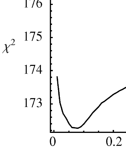
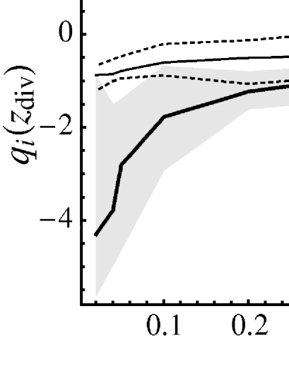
We now illustrate the exploration that identifies the optimal bin arrangement for fixed $N_{\mathrm{p}}$. Fig. 1 shows the dependence of $\chi^{2}$ on the bin boundary position $z_{\mathrm{div}}$ for $N_{\mathrm{p}}=2$ models. We identify the model with $z_{\mathrm{div}}=0.08$ as the one with a smaller $\chi^{2}$ and label it as the ‘optimized model’. Large-$\chi^{2}$ (worse fit) models are limiting cases resembling the constant $w$ model, their $\chi^{2}$ and preferred $w_{1}$ values tend to the ones of the single-parameter case (later shown in Table 1). This is not surprising if we bear in mind that $95\%$ of SNe belong to the first redshift bin when $z_{\mathrm{div}}\sim 1$.

Figure 1: Dependence of $\chi^{2}$ on the bin boundary $z_{\mathrm{div}}$ that characterizes LPC models with two segments.

Table 1: Parameter estimates together with $\chi^{2}$ and BIC values for various models. The difference $\Delta$BIC is calculated with respect to the base model $\Lambda$CDM. Redshift arrangements are shown for our optimized models.

Model	Optimized $\{z_{\mathrm{div}}\}$	$w_{0}$	$w_{a,z}$	$q_{1}$	$q_{2}$	$q_{3}$	$q_{4}$	$q_{5}$	$\chi^{2}_{\mathrm{min}}$	BIC	$\Delta$BIC
$\Lambda$CDM		$\equiv$-1							178.6	178.6	0.0
$N_{\mathrm{p}}=1$				-0.90					177.9	182.9	4.4
$N_{\mathrm{p}}=2$	$\{0.08\}$			-2.05	-0.60				172.7	182.8	4.3
$N_{\mathrm{p}}=3$	$\{0.43,0.60\}$			-1.08	2.01	-1.90			171.2	186.4	7.8
$N_{\mathrm{p}}=4$	$\{0.05,0.55,0.70\}$			-3.56	-0.63	7.45	-25.01		170.5	190.7	12.1
$N_{\mathrm{p}}=5$	$\{0.05,0.50,0.60,0.70\}$			-3.62	-0.67	9.80	-3.94	-40.16	169.6	194.8	16.3
eq. err.	$\{0.18\}$			-1.28	-0.46				173.4	183.5	4.9
$w\propto a$		-1.32	2.61						173.8	183.9	5.3
$w\propto z$		-1.27	1.63						174.3	184.4	5.8

Figure 2: (color online) The optimized $N_{\mathrm{p}}=2$ model. Top: Likelihoods for the optimized 2-parameter model. Note that the low-redshift estimate (red/gray line) is broader than the medium- and large-redshift estimate (black line). Color conventions are the same for the three plots. Middle: Uncorrelated principal component estimates of $w(z)$ (thin, horizontal lines) with corresponding 1-$\sigma$ (solid) and 2-$\sigma$ (dotted) rectangles showing parameter constraints (horizontal edges) and redshift span (vertical edges). Bottom: Window functions relating original piecewise coefficients to LPC ones.

In Table 1 we present the models obtained by means of optimization for $N_{\mathrm{p}}=1-5$, together with the base model $\Lambda$CDM and two other parametrizations commonly used in the literature: $w(z)=w_{0}+w_{z}z$ wz and $w(a)=w_{0}+w_{a}(1-a)$ wa . We also include the model selection quantity $\Delta$BIC, all statistics are obtained using the Gold dataset.

Model comparison in light of the BIC criterion shows that $\Lambda$CDM is the model preferred by data. A collection of models that exhibit low $\chi^{2}$ but are moderately disfavored are $N_{\mathrm{p}}=1$, $N_{\mathrm{p}}=2$, $w\propto z$, $w\propto a$ and the equal errors model explained below. The $N_{\mathrm{p}}=3$ model turns out to be strongly disfavored while $N_{\mathrm{p}}=4$ and $N_{\mathrm{p}}=5$ are decidedly disfavored, all this in terms of the rules proposed in KR .

It is worth mentioning that all time-varying $w$ models, favored by the BIC or not, suggest a principal component value $q_{1}<-1$ at low redshifts. The table also suggests that a larger number of LPC estimates implies more extreme values for $q_{i}$. This reminds of certain parametrizations that, when extended to second order expansions, acquire huge values in their expansion coefficients, as studied in BCK . We won’t be concerned by the huge values found, since the models in question are already rejected by the BIC criterion. Still, it is somewhat disconcerting that the further redshift divisions are added, estimates are more and more inconsistent with $q_{1}\sim-1$.

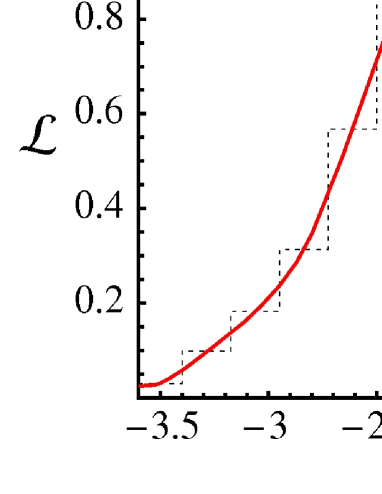
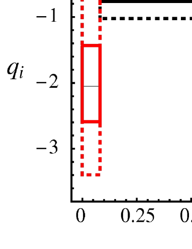
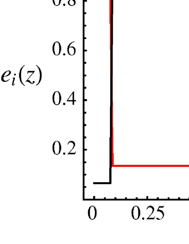
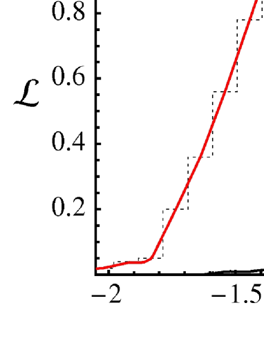
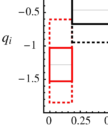
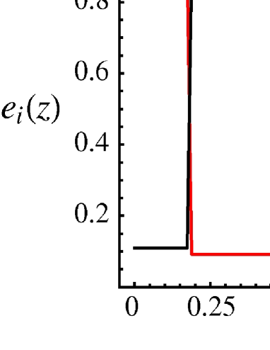
A more detailed analysis of the optimized $N_{\mathrm{p}}=2$ case shows that $q_{1}$ is loosely constrained with respect to $q_{2}$. This is illustrated in Figure 2, where likelihoods (top plot) and constraints on model parameters $q_{i}$ (middle plot) are shown. The bottom plot of the figure shows the highly localized, mostly positive window functions resulting from the LPC approach.

An alternative $N_{\mathrm{p}}=2$ model is obtained by a different optimization criterion which, instead of accepting the model with minimum $\chi^{2}$, requires errors in parameter estimates to be of comparable size. This case exemplifies how different optimization criteria may result in different $w$-estimates. In figure 3 we sketch the interplay between $q_{1}$ and $q_{2}$ estimates when $z_{\mathrm{div}}$ is varied. A detailed analysis points to the $z_{\mathrm{div}}=0.18$ model as the one with matching errors, which is labeled the equal errors model. As seen in Table 1, this model has practically the same BIC value as the $N_{\mathrm{p}}=1$ and $N_{\mathrm{p}}=2$ models. Its corresponding likelihood, parameter estimates and window functions are plotted in Figure 4.

It is interesting that two of the models with good fits to the data, the optimized $N_{\mathrm{p}}=2$ and equal errors ones, are reminiscent of some more complex models —for example the ones in BCK ; HC ; mod — which suggest $w<-1$ at low redshift and $w\sim-0.5$ elsewere. However, our models rely on two parameters only, which makes them more attractive in terms of model selection, making a better case for the rapidly varying $w$ possibility.

Figure 3: Parameter estimates $q_{1}$ (thick line) and $q_{2}$ (thin line) for varying $z_{\mathrm{div}}$ and their corresponding 2$\sigma$ confidence regions.

Figure 4: (color online) The equal errors model, a 2-parameter model similar to the optimized one but with comparable errors on both $q$-estimates. Likelihoods (top), $q$-estimates describing $w(z)$ (middle) and window functions (bottom) are displayed following the color coding of Figure 2.

IV Conclusions

This paper introduces a new framework to study the model-independent implications of data regarding the possibility of dark energy evolution. Extending the approach proposed in HC , we find the optimal set of eigenfunctions that describe $w$. We focus on a currently available SNe dataset gold , and follow a model selection scheme, in terms of the Bayesian information criterion, which points to $\Lambda$CDM as the preferred model. A class of models is found to provide better fits to data but is moderately disfavored by the BIC. These include our two-parameter models: the one that minimizes $\chi^{2}$ and the one with equal errors on both estimates, as well as the constant $w$ parametrization. Also in this category, with slightly worse BIC values, are the ‘linear in redshift’ and ‘linear in scale factor’ parametrizations. Optimized models with more than two parameters are strongly disfavored.

In the light of the data considered, mutually exclusive phenomenologies are found to be equally favored by the BIC, for example, the constant $w$ and optimized $N_{\mathrm{p}}=2$ models which are, respectively, consistent and marginally consistent with $\Lambda$CDM at a 95$\%$ confidence level. This reproduces a problem commonly found in the literature when considering flexible forms of $w(z)$: the constant $w$ model leads to $w\sim-1$ at all redshifts, but if $w$ is allowed to evolve we find that $w<-1$ at low redshift and $w>-1$ elsewhere. Our approach may prove useful in reconstructing a true model with a rapidly varying $w$, however, current data give no information on whether this option is preferred over a slowly varying or constant $w$, even when the rapidly varying $w$ is described with a simple model such as our two-parameter ones.

Interpretation of the favored models should be made while considering that resulting estimates are “integrated properties of w(z)” SPB , and so the underlaying physical model may differ substantially from the reconstructed one. In particular, the $z_{\mathrm{div}}$ found in our optimized models is not necessarily a proof of change in dark energy dynamics at exactly that time, it could be seen as a feature of the reconstruction employed.

Further research, adding other observational tests to the analysis, may improve constraints on the equation of state. Of special interest are weak lensing measurements wl , or the observed Integrated Sachs-Wolfe effect SW , which for certain cases provides a probe of the total change in $w$ PCSCN . This is postponed for a future investigation.

Appendix A

In this appendix we show, following HC , the procedure to decompose $w$ in terms of localized principal components.

We first calculate the Fisher matrix $\mathbf{F}$ TTH (marginalized over nuisance parameters) for some $w$ model and with respect to a given dataset. We then obtain its square root

$$\mathbf{F}^{1/2}=\mathbf{O}^{\mathrm{T}}\sqrt{\mathbf{\Lambda}}\mathbf{O},$$ (7)

where the diagonalized matrix of eigenvalues $\mathbf{\Lambda}$ and the orthogonal matrix of eigenvectors $\mathbf{O}$ satisfy

$$\mathbf{F}=\mathbf{O}^{\mathrm{T}}\mathbf{\Lambda}\mathbf{O}.$$ (8)

It is straightforward to check that $\mathbf{F}^{1/2}$ is indeed the ‘square root matrix’ of $\mathbf{F}$ if we consider the product $\mathbf{F}^{1/2}\mathbf{F}^{1/2}$.

LPC estimates $\mathbf{q}$ are given in terms of the original parameters $\mathbf{p}$ by $\mathbf{q}=\mathbf{W}\mathbf{p}$, where $\mathbf{W}$ is a normalized version of $\mathbf{F}^{1/2}$ for which each row adds up to 1 (Roman indices run from 1 to $N_{\mathrm{p}}$ and summations are explicitely shown):

$$W_{ij}=\frac{F^{1/2}_{ij}}{\sum_{k}\limits F^{1/2}_{ik}}.$$ (9)

The rows of $W$ then define the window functions $\mathbf{e}$ which provide the desired orthogonal basis. Furthermore, when considering the covariance of the original parameters $\langle\Delta p_{i}\Delta p_{j}\rangle=F^{-1}_{ij}$ and the diagonality of $W$, the new errors $\Delta q_{i}$ are found to be uncorrelated, their covariance being

$$\langle\Delta q_{i}\Delta q_{j}\rangle=\frac{\delta_{ij}}{\sum_{k}\limits F^{1/2}_{ik}\sum_{l}\limits F^{1/2}_{jl}}.$$ (10)

Our expansion in terms of the window functions is then written as:

$$w(z)=\sum_{i}q_{i}\,e_{i}(z),$$ (11)

where instead of ordering the principal components, as is usual, according to the magnitude of individual uncertainties, we respect the original indexing to maintain the transparency of the interpretation.

References

- (1) A. Riess et al., Astron. J. 116,1009 (1998); S. Perlmutter et al., Astrophys. J. 517, 565 (1999).
- (2) M. Tegmark et al. [SDSS Collaboration], Phys. Rev. D 69, 103501 (2004).
- (3) B. A. Bassett, P. S. Corasaniti and M. Kunz, Astrophys. J. 617, L1 (2004).
- (4) I. Maor, R. Brustein, J. McMahon and P.J. Steinhardt, Phys. Rev. D 65, 123003 (2002).
- (5) A. Melchiorri, L. Mersini-Houghton, C. J. Odman and M. Trodden, Phys. Rev. D 68, 043509 (2003).
- (6) D. Huterer and G. Starkman, Phys. Rev. Lett. 90, 031301 (2003).
- (7) D. Huterer and A. Cooray, Phys. Rev. D 71, 023506 (2005).
- (8) E. V. Linder and D. Huterer, Phys. Rev. D 72, 043509 (2005).
- (9) R. G. Crittenden and L. Pogosian, arXiv:astro-ph/0510293.
- (10) C. Shapiro and M. S. Turner, arXiv:astro-ph/0512586.
- (11) M. Tegmark, Phys. Rev. D 66, 103507 (2002).
- (12) M. Tegmark, Phys. Rev. D 55, 5895 (1997).
- (13) E. V. Linder and D. Huterer, Phys. Rev. D 67, 081303 (2003).
- (14) T. D. Saini, J. Weller and S. L. Bridle, Mon. Not. Roy. Astron. Soc. 348, 603 (2004).
- (15) D. N. Spergel et al., arXiv:astro-ph/0603449.
- (16) T. R. Choudhury and T. Padmanabhan, Astron. Astrophys. 429, 807 (2005).
- (17) A. G. Riess et al. [Supernova Search Team Collaboration], Astrophys. J. 607, 665 (2004).
- (18) A. R. Liddle, Mon. Not. Roy. Astron. Soc. 351, L49 (2004).
- (19) G. Schwarz, Annals of Statistics 6, 461 (1978).
- (20) M. Sahlén, A. R. Liddle and D. Parkinson, Phys. Rev. D 72, 083511 (2005); W. Godlowski and M. Szydlowski, Phys. Lett. B 623, 10 (2005); M. Szydlowski and A. Kurek, arXiv:astro-ph/0603538.
- (21) see, for example, D. J. C. MacKay, Information theory, inference and learning algorithms, Cambridge University Press (2003).
- (22) R. E. Kass and A. E. Raftery, J. Amer. Stat. Assoc. 90, 773 (1995).
- (23) A. R. Cooray and D. Huterer, Astrophys. J. 513, L95 (1999).
- (24) M. Chevallier and D. Polarski, Int. J. Mod. Phys. D10, 213 (2001); E.V. Linder, Phys. Rev. Lett. 90, 091301 (2003).
- (25) U. Alam, V. Sahni, T. D. Saini and A. A. Starobinsky, Mon. Not. Roy. Astron. Soc. 354, 275 (2004); S. Hannestad and E. Mortsell, JCAP 0409, 001 (2004).
- (26) T. D. Saini, T. Padmanabhan and S. Bridle, Mon. Not. Roy. Astron. Soc. 343, 533 (2003).
- (27) See, for example, W. Hu and M. Tegmark, Astrophys. J. 514, L65 (1999); D. Huterer, Phys. Rev. D 65, 063001 (2002); B. Jain and A. Taylor, Phys. Rev. Lett. 91, 141302 (2003).
- (28) R. K. Sachs and A. M. Wolfe, Astrophys. J. 147, 73 (1967),
- (29) L. Pogosian, P. S. Corasaniti, C. Stephan-Otto, R. Crittenden and R. Nichol, Phys. Rev. D 72, 103519 (2005).
- (30) M. Tegmark, A. N. Taylor and A. F. Heavens, Astrophys. J. 480, 22 (1997).