Searching for modified gravity with baryon oscillations: from SDSS to wide field multiobject spectroscopy (WFMOS)

Abstract

We discuss how the baryon acoustic oscillation (BAO) signatures in the galaxy power spectrum can distinguish between modified gravity and the cosmological constant as the source of cosmic acceleration. To this end we consider a model characterized by a parameter $n$, which corresponds to the Dvali-Gabadadze-Porrati (DGP) model if $n=2$ and reduces to the standard spatially flat cosmological constant concordance model for $n$ equal to infinity. We find that the different expansion histories of the modified gravity models systematically shifts the peak positions of BAO. A preliminary analysis using the current SDSS LRG sample indicates that the original DGP model is disfavored unless the matter density parameter exceeds $0.3$. The constraints will be strongly tightened with future spectroscopic samples of galaxies at high redshifts. We demonstrate that WFMOS, in collaboration with other surveys such as Planck, will powerfully constrain modified gravity alternatives to dark energy as the explanation of cosmic acceleration.

I Introduction

Exploring the origin of the cosmic acceleration is one of the most challenging problems in cosmology. The nature of the cosmic expansion history can be investigated using a variety of cosmological observations: the anisotropies in the cosmic microwave background at $z=1100$, the Hubble diagram of supernovae, cosmic shear statistics of galaxies with photometric redshifts, and spatial clustering of galaxies with spectroscopically measured redshifts. In the present paper, we focus on the fourth method which relies on extracting the baryon acoustic oscillations (BAO) in the high-z galaxy power spectrum eis ; Blake ; LinderA ; SE ; HH ; Amendola .

Recently the clear detection of the baryon oscillations has been reported Eisenstein ; Cole ; Huetsi ; Yahata already yielding some constraints surely on dark energy and particularly cosmic curvature. Based on this success, and the fact that the systematic errors in the BAO method appear easier to control (due to the fact that the characteristic scale of  100 Mpc is fundamentally linear), many BAO projects for the future are being discussed. For example, the AAOmega spectrograph on the 2dF system will be able to observe a large number of galaxies in the range of redshift $0.5<z<0.9$ AAOmega . The Fibre Multi Object Spectrograph (FMOS) on Subaru will be able to measure redshifts of more than $6\times 10^{5}$ Ly-$\alpha$ emitting galaxies around $z=1.5$ in near future Totani . The Large sky Area Multi-Object fiber Spectroscopic Telescope (LAMOST) project in China has a capability of performing large redshift-survey Lamost , while HETDEX (Hobby-Eberly Telescope Dark Energy Experiment) aims to measure redshifts of more than $10^{6}$ Ly-$\alpha$ emitting galaxies using VIRUS (Visible Integral-field Replicable Unit Spectrograph) HETDEX . Furthermore, on a longer timescale, very large galaxy surveys might be performed with a space-based telescope JEDI and the SKA radio telescope SKA .

In this paper we concentrate on the constraints that can be expected from the planned WFMOS. It is a BAO survey that aims to measure the redshift of more than two millions of high-z galaxies with a large field of view and multi-fiber spectrograph ( 4000 fibers) on a large ground-based telescope such as Subaru WFMOS . While the optimal geometry of WFMOS is not finalized yet we will use the fiducial baseline concept. One aim of the present paper is to demonstrate the power of WFMOS to extract the baryon oscillation in the galaxy power spectrum and the resulting tests that can be made of modified gravity models which are putative explanations for the acceleration of the cosmos.

Although the cosmological constant is the simplest model leading to acceleration, new dynamical degrees of freedom (e.g., a scalar field) with effective negative pressure may be the source of acceleration. An interesting possibility is that acceleration results not from an additional repulsive force but through the weakening of traditional Einstein gravity on very large scales. The archetypal model in this class is the Dvali-Gabadadze-Porrati (DGP) model which was developed in the context of the brane world scenario, which includes a mechanism to explain self-acceleration in the late time universe DGP ; Gabadadze . The DGP model and variants Lue ; Fairbairn ; Alam ; Maartens will serve as a testbed for testing the ability of WFMOS to distinguish them from a cosmological constant. We note here that the DGP model is not without subtleties and problems at the quantum level as discussed in Luty ; Nicolis ; ghostkoyama .

Very recently, the evolution of the large-scale cosmological perturbations of the DGP cosmological model have been studied in detail with rather general assumptions km compared to earlier works Song ; Carroll ; LSS . Koyama has also presented a generalized model that interpolates between the DGP model and the CDM model with a cosmological constant ($\Lambda$CDM) in general relativity sfk . We will see that WFMOS may well provide not only a chance to test dark energy models but also to put general relativity to severe tests on large scales. To achieve this we investigate the theoretical predictions of modified gravity models in the galaxy power spectrum from a survey with WFMOS.

So far, there are a few works which focus on the nature of the large scale structure in a modified gravity model Sealfon ; Nusser ; Shirata . In the present paper, we consider the DGP cosmological model and its variants from the point of view of testing the gravity theory with the baryon oscillation, and investigate a future prospect assuming the WFMOS project for the first time. We also investigate the current consistency with observation utilizing the power spectrum. A similar problem is considered in Maartens ; Guo ; SSH , however, these works make use of a result on the distance from the SDSS LRG correlation function analysis in Eisenstein .

This paper is organized as follows: In section 2, a brief review of the DGP cosmological model and its variants is presented. In section 3, our theoretical modeling of the power spectrum and our basic statistic is explained. Then, a current comparison of the theoretical model with the observational result with the luminous red galaxy (LRG) sample in the SDSS is presented in section 4. In section 5, we discuss the baryon oscillation features, assuming a future WFMOS sample, as a test of the modified gravity model. We discusses how one can improve the constraints on modified gravity models from future WFMOS samples. The last section is devoted to a summary and conclusions. Throughout this paper, we use units in which the speed of light and the Planck constant are unity, $c=\hbar=1$. We adopt the Hubble parameter: $H_{0}=72~{}{\rm km/s/Mpc}$, unless we mention explicitly.

II The DGP cosmological model and variants

We start with a brief review of the DGP cosmological model (see e.g., Gabadadze ). The DGP model is based on the brane world scenario, and is constructed by embedding a (3+1)dimensional brane in a (4+1)dimensional bulk with infinite volume, with action

$$S=-{M_{*}^{3}\over 16\pi}\int d^{5}X\sqrt{-g^{(5)}}R^{(5)}-{M_{\rm pl}^{2}\over 16\pi}\int d^{4}x\sqrt{-g^{(4)}}R^{(4)}+\int d^{4}x\sqrt{-g^{(4)}}{\cal L}_{m}+S_{\rm G.H.},$$ (1)

where $M_{*}$ ($M_{\rm pl}$) is the fundamental Planck mass in the 5-dim (4-dim) space-time, $g^{(5)}$ ($g^{(4)}$) and $R^{(5)}$ ($R^{(4)}$) denote the determinant and the Ricci scalar of the 5-dim (4-dim) metric, respectively, and ${\cal L}_{m}$ is the matter Lagrangian on the brane. The final term, the Hawking-Gibbons term $S_{G.H.}$, is added so as to reproduce the appropriate field equation in a space-time with a boundary. The term with $R^{(4)}$ in the above action is assumed to be induced by quantum effects in the matter sector on the brane.

The crucial cross-over scale, $r_{c}$, is defined by the ratio of the Planck scales

$$r_{c}=\frac{M_{\rm pl}^{2}}{2M_{*}^{3}}.$$ (2)

This characterizes the region where gravity switches from being 4-dimensional (scales less than $r_{c}$) to being 5-dimensional (scales greater than $r_{c}$) which causes a modification of the laws of gravity on cosmologically larger scales if $r_{c}\sim H_{0}^{-1}$. As a result so-called self-acceleration may appear. The cosmological solution of the DGP model give

$$H^{2}-\frac{H}{r_{c}}=\frac{8\pi\rho}{3M_{\rm pl}^{2}},$$ (3)

where $H(t)$ is the Hubble expansion rate, $\rho(t)$ is the matter density, and $M_{\rm pl}^{-2}$ is regarded as the 4-dimensional gravitational constant, $G$.

Cosmological perturbations have also been studied in the modified DGP-like models sfk , originally proposed by Dvali and Turner DT . These variants are phenomenological models interpolating between the DGP model and $\Lambda$CDM. Adopting this modified DGP-like model, the modified Friedmann equation is

$$H^{2}-{H^{2/n}\over r_{c}^{2-2/n}}={8\pi\rho\over 3M_{\rm pl}^{2}},$$ (4)

where $r_{c}$ and $n$ are the parameters of the model. In this paper, we assume spatially flat sections, implying that the parameter $r_{c}$ is related to the cosmological parameters by $(H_{0}r_{c})^{2/n-2}=1-\Omega_{m}$, where $\Omega_{m}$ is the matter density parameter.

This model is the DGP model for $n=2$, and it reduces to $\Lambda$CDM for $n\rightarrow\infty$. Following the analysis of the modified DGP-like modelsfk , the evolution equation for the linear density perturbation (linear growth factor) obeys

$$\ddot{D_{1}}+2H\dot{D_{1}}={4\pi\over M_{\rm pl}^{2}}\left(1+{1\over 3\beta}\right)\rho{D_{1}},$$ (5)

where

$$\beta=1-n(Hr_{c})^{2(n-1)/n}\left(1+{2(n-1)\dot{H}/3nH^{2}}\right).$$ (6)

In the present paper, we test these modified DGP models by extracting the baryon oscillations of simulated and real galaxy power spectra.

Concerning the linear growth factor, the time evolution slightly depends on the treatment and assumptions of the perturbation equation km ; Song ; Carroll ; LSS ; sfk . However, the difference is small, and the effect on the baryon oscillation feature is negligible in the cases studied in the present paper. In a strict sense, the growth factor is the expression under the sub-horizon approximation. Hence the growth factor may depend on wavenumber at large scales, which could lead to additional scale dependence KKprivate .

III Baryon acoustic oscillation in the modified DGP model: theoretical predictions in linear theory

The reason why clustering statistics are sensitive to the expansion history of the universe comes primarily from the baryon acoustic oscillations (BAO), which imprints a characteristic scale on the galaxy distribution that acts as a standard ruler, which we briefly summarize here (see also e.g. eis ; Blake ; LinderA ; SE ; HH ; Amendola ). The origin of the BAO in the matter power spectrum can be understood as the velocity fluctuation of the baryon fluid at the decoupling time EH ; MWP . The characteristic scale of the baryon oscillation is determined by the sound horizon at decoupling, which depends on the total matter density and baryon densities. Because we can measure this scale in both the transverse and radial directions the BAO yields both the angular diameter distance and Hubble parameter at that redshift. Thus, the precise measurement of the BAO scale from galaxy power spectrum can put important constraints on the cosmic expansion history.

Our model predictions of galaxy power spectra in the modified DGP model proceed as follows (see Suto ; Y2003 for details). In the linear regime, the real-space mass power spectrum $P_{\rm mass}(q;z)$ is translated to the galaxy power spectrum in redshift-space as

$$P_{\rm gal}({q_{\scriptscriptstyle\|}},{q_{\scriptscriptstyle\bot}};z)=b^{2}(z)\left[1+\frac{1}{b(z)}\frac{d\ln D_{1}(z)}{d\ln a(z)}\left(\frac{q_{\scriptscriptstyle\|}}{q}\right)^{2}\right]^{2}P_{\rm mass}(q;z),$$ (7)

where $a(z)$ is the scale factor at $z$, $q_{\scriptscriptstyle\|}$ and $q_{\scriptscriptstyle\bot}$ is the parallel and perpendicular component of the comoving wavenumber to the line-of-sight direction. We assume a linear scale-independent galaxy bias, $b(z)$.

Mapping the length scale from the observed distribution, i.e., redshift and angular separations $\delta z$ and $\delta\theta$, becomes sensitive to the cosmological parameters at high redshiftsAP ; Ballinger ; MatsubaraSuto . If one adopts a fiducial set of cosmological parameters in estimating the power spectrum from the observed galaxy distribution, the result is necessarily distorted from the actual spectrum, but the effect can be modeled theoretically. Suppose that the Hubble parameter in the fiducial model is $H^{\rm(f)}(z)$ instead of the true one, $H(z)$, which can be obtained by numerically solving the modified Friedman equation (4). Then, comoving radial distances in the fiducial and true universes are given by

$$r^{\rm(f)}(z)=\int_{0}^{z}\frac{dz^{\prime}}{H^{\rm(f)}(z^{\prime})},\qquad r(z)=\int_{0}^{z}\frac{dz^{\prime}}{H(z^{\prime})}.$$ (8)

The parallel and perpendicular comoving distances that correspond to the observables $\delta z$ and $\delta\theta$, respectively, are

$$x_{\scriptscriptstyle\|}=\frac{dr(z)}{dz}\delta z=\frac{1}{H(z)}\delta z,\qquad x_{\scriptscriptstyle\bot}=r(z)\delta\theta.$$ (9)

Therefore their counterparts in the model universe with the adopted fiducial parameters are related to the above as

$$x^{\rm(f)}_{\scriptscriptstyle\|}=\frac{H(z)}{H^{\rm(f)}(z)}x_{\scriptscriptstyle\|},\qquad x^{\rm(f)}_{\scriptscriptstyle\bot}=\frac{r^{\rm(f)}(z)}{r(z)}x_{\scriptscriptstyle\bot}.$$ (10)

The corresponding relations for the wavenumbers read

$$k^{\rm(f)}_{\scriptscriptstyle\|}=\frac{H^{\rm(f)}(z)}{H(z)}q_{\scriptscriptstyle\|}\equiv k^{\rm(f)}\mu,\qquad k^{\rm(f)}_{\scriptscriptstyle\bot}=\frac{r(z)}{r^{\rm(f)}(z)}q_{\scriptscriptstyle\bot}\equiv k^{\rm(f)}\sqrt{1-\mu^{2}},$$ (11)

which yield

$$q^{2}={q_{\scriptscriptstyle\|}}^{2}+{q_{\scriptscriptstyle\bot}}^{2}=[k^{\rm(f)}]^{2}\left[\mu^{2}\left(\frac{H(z)}{H^{\rm(f)}(z)}\right)^{2}+(1-\mu^{2})\left(\frac{r^{\rm(f)}(z)}{r(z)}\right)^{2}\right].$$ (12)

Then, the power spectrum in the fiducial universe is computed from

$$P^{\rm(f)}(k^{\rm(f)},\mu,z)d^{2}k^{\rm(f)}_{\scriptscriptstyle\bot}dk^{\rm(f)}_{\scriptscriptstyle\|}=P_{\rm gal}({q_{\scriptscriptstyle\|}},{q_{\scriptscriptstyle\bot}};z)d^{2}q_{\scriptscriptstyle\bot}dq_{\scriptscriptstyle\|}.$$ (13)

Combining equations (7), (11), and (12), one obtains

$$P^{\rm(f)}(k^{\rm(f)},\mu,z) = b^{2}(z)\left[1+\frac{1}{b(z)}\frac{d\ln D_{1}(z)}{d\ln a(z)}\left\{\mu^{2}+(1-\mu^{2})\left(\frac{H^{\rm(f)}(z)r^{\rm(f)}(z)}{H(z)r(z)}\right)^{2}\right\}^{-1}\right]^{2}\left[\frac{H(z)}{H^{\rm(f)}(z)}\right]\left[\frac{r^{\rm(f)}(z)}{r(z)}\right]^{2}$$ (14)

$$\times P_{\rm mass}\left(k^{\rm(f)}\sqrt{\mu^{2}\left(\frac{H(z)}{H^{\rm(f)}(z)}\right)^{2}+(1-\mu^{2})\left(\frac{r^{\rm(f)}(z)}{r(z)}\right)^{2}};z\right).$$ (15)

Finally, the estimated power spectrum is given by integrating equation (14) over the light-cone:

$$P(k)=\frac{\displaystyle\int_{0}^{1}d\mu\int_{z_{\rm min}}^{z_{\rm max}}dz{dr^{\rm(f)}(z)\over dz}r^{\rm(f)}(z)^{2}\bar{n}(z)^{2}\psi(z,k)^{2}P^{\rm(f)}(k,\mu;z)}{\displaystyle{\int_{z_{\rm min}}^{z_{\rm max}}dz{dr^{\rm(f)}(z)\over dz}r^{\rm(f)}(z)^{2}\bar{n}(z)^{2}\psi(z,k)^{2}}},$$ (16)

where we write $k^{\rm(f)}$ simply as $k$. The mean number density of galaxies in the cosmological redshift space, $\bar{n}(z)$, is not directly observable, but rather inferred from the observed number count $dN(z)/dz$:

$$\frac{dN}{dz}=\bar{n}(z)\frac{[r^{\rm(f)}(z)]^{2}}{H^{\rm(f)}(z)}.$$ (17)

We may introduce a weight factor, $\psi(z,k)$, which is set as $1/[1+P(k,\mu,z)\bar{n}(z)]$ in the optimal weighting scheme. In the present paper, we adopt $\psi(z,k)=1/\bar{n}(z)$ for the SDSS LRG sample following ref.Huetsi , and $\psi(z,k)=1$ for future WFMOS samples for simplicity.

The analysis presented in this paper focuses on the local power-law index of the power spectrum:

$${d\ln P(k)\over d\ln k}={1\over P(k)}{dP(k)\over d\ln k}.$$ (18)

In general, ${d\ln P(k)/d\ln k}$ does not contain all the information encoded in $P(k)$ so constraints from ${d\ln P(k)/d\ln k}$ will be somewhat weaker than those from $P(k)$. However, ${d\ln P(k)/d\ln k}$ may be useful in extracting the baryon oscillation feature because, as long as the oscillations are clearly detected the principal part of the constraints on the cosmic expansion history using the power spectrum come from the oscillations sesim . In addition, ${d\ln P(k)/d\ln k}$ does not depend on the amplitude of the power spectrum. Thus, it is not sensitive to the bias and the growth factor which provides a desirable level of model-independence. In our theoretical predictions, we obtain $d\ln P(k)/d\ln k$ by differentiating $P(k)$ with respect to $k$ which does introduce some level of additional noise.

The fiducial cosmological model that we choose in the following analysis is a spatially-flat $\Lambda$ CDM with $\Omega_{m}^{\rm(f)}=0.27$, $\Omega_{\Lambda}^{\rm(f)}=1-\Omega_{m}^{\rm(f)}$, $\Omega_{b}=0.044$, and $h=0.72$. Therefore

$$H^{\rm(f)}(z)=H_{0}\sqrt{\Omega_{m}^{\rm(f)}(1+z)^{3}+1-\Omega_{m}^{\rm(f)}}.$$ (19)

Since we assume scale-independent linear growth factor in the modified DGP model (eq.[5]), $P_{\rm mass}(q;z)$, except for its overall amplitude, is exactly the same as that in the fiducial $\Lambda$CDM model. The spectrum is computed using the linear transfer function by Eisenstein and Hu EH , and the primordial spectral index $n_{s}=0.95$ and $\sigma_{8}=0.8$ WMAP . For definiteness we adopt $\psi(k,z)=1$, and the Fry’s bias model:

$$b(z)=1+\frac{b_{0}-1}{D_{1}(z)}$$ (20)

with $b_{0}=1.5$ for the samples WFMOS1 and WFMOS2, and with $b_{0}=2$ for the sample SDSS LRG (see below for details). The reasonable change in the bias model does not alter our results for $d\ln P(k)/d\ln k$. However the error does depend on the bias amplitude.

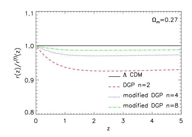
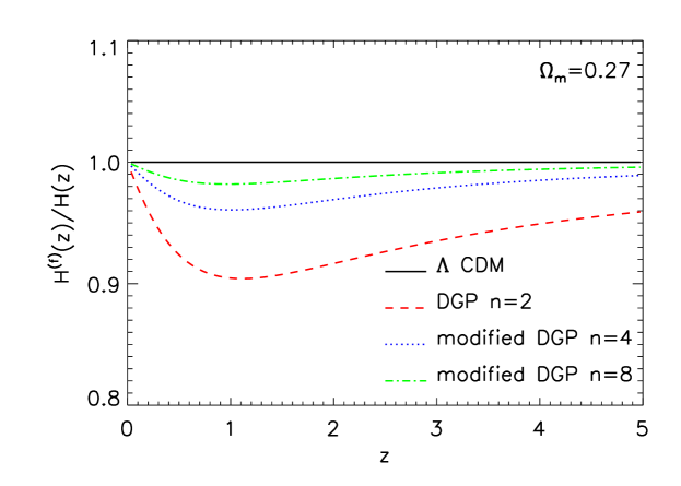
Figs. 1 and 2 plot $r(z)/r^{(f)}(z)$ and $H^{(f)}(z)/H(z)$, respectively, as function $z$ for the original DGP model ($n=2$; the dashed curve), and the modified DGP models with $n=4$ (dotted curve) and $n=8$ (dash-dotted curve). Here the density parameter is fixed as $\Omega_{m}=0.27$. The solid curve is the $\Lambda$CDM model, which is trivially $r(z)/r^{(f)}(z)=H^{(f)}(z)/H(z)=1$, because it is equivalent to the fiducial model. For clearly differentiating models, the deviation of $r(z)/r^{(f)}(z)$ and $H^{(f)}(z)/H(z)$ from unity is important. Therefore, the sample of the redshift larger than 0.5 is effective for selecting the models.

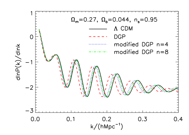
In the rest of this section, we consider theoretical predictions of the modified gravity model for $d\ln P(k)/d\ln k$. Here we assume a future fiducial WFMOS survey in the range of redshifts $0.5<z<1.3$ ($z_{\rm min}=0.5$ and $z_{\rm max}=1.3$; see section 5 for details). Fig. 3 shows the theoretical curves of ${d\ln{P}/d\ln k}$ for the original DGP model ($n=2$, dashed curve), the DGP-like models with $n=4$ and $n=8$ (dotted and dashed-dotted curves) and for the $\Lambda$CDM model (solid curve, the fiducial model). We have fixed the spectral index of the initial spectrum to the value $n_{s}=0.95$ and the density parameters to $\Omega_{b}=0.044$, $\Omega_{m}=0.27$. The difference of predictions between the fiducial $\Lambda$ CDM model and the modified gravity models entirely comes from the geometric distortion, i.e., the model-dependent relation between $q$ and $k$, equation (11). The apparent geometric distortion disappears only when the actual universe has the same $H^{\rm(f)}(z)$ and $r^{(f)}(z)$ for $z<z_{\rm max}$ of the fiducial model.

It is instructive to consider how the theoretical predictions are sensitive to the cosmological parameters in order to understand the degeneracy among different parameters. For this purpose, we plot the results for different $\Lambda$ CDM models by varying the values of $\Omega_{m}$ and $\Omega_{b}$ in Figs. 4 and 5, while the other parameters are the same as the fiducial $\Lambda$ CDM model in Fig. 3. Note again that the wavenumber $k$ in Figs. 4 and 5 is also computed under the assumption of the fiducial model parameters and should be regarded as $k^{\rm(f)}$.

Figs. 4 and 5 indicate that varying $\Omega_{m}$ and $\Omega_{b}$ in spatially-flat CDM models mainly affects the amplitude of the BAO, but the induced shift of the peak positions is weak, at least much weaker than the difference between the DGP model and the fiducial model illustrated in Fig. 3. This also applies to the change of the spectral index, $n_{s}$. Therefore we conclude that the degeneracy among those parameters space is not so crucial, although it is clear that a prior constraint on these parameters is important and complementary to the BAO test.

IV Current constraints: SDSS LRG sample

In this section, we utilize the theoretical framework developed in the previous section to place constraints on modified DGP models from existing large–scale structure data. For this purpose, we use the published power spectrum of galaxy clustering by H$\ddot{\rm u}$tsi Huetsi based on 51763 LRGs from Data Release Four (DR4) of the Sloan Digital Sky Survey (SDSS). In this work, they present a discovery of the BAO in the power spectrum and compute the covariance matrix as well, which is ideal to apply our current methodology.

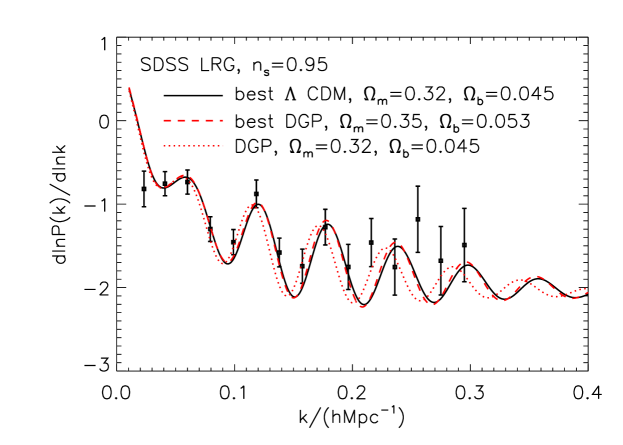
We fit our cosmological models to the power spectrum data by varying $\Omega_{m}$ and $\Omega_{b}$, assuming spatial flatness both for the $\Lambda$CDM and modified DGP models. In Figure 6, we present the best fit $\Lambda$ CDM model (solid line) and the best fit DGP model (dashed line) to the SDSS LRG power spectrum of Huetsi . For comparison, we also present the predicted DGP model (dotted line) with the same cosmological parameters as the best fit $\Lambda$ CDM model, i.e., with $\Omega_{m}=0.32$ and $\Omega_{b}=0.045$. For these fits, we have used $z_{\rm min}=0.16$ and $z_{\rm max}=0.47$, as well as determined the comoving number density $\bar{n}(z)$ (see Fig. 4 of Huetsi ) in the fiducial model cosmology (assuming the first year WMAP parameters). The error bars were computed via Monte Carlo simulations and the covariance matrix provided by Huetsi . To minimize non–linear effects, we only fit to the SDSS LRG power spectrum at scales of $k<0.2~{}h{\rm Mpc}^{-1}$. When quasi-nonlinear effects properly taken accounted forSS ; MSS ; MWP ; JK , we may increase the range of scales used in this analysis and thus improve the statistics.

In Figure 7 (a), we show the contours of $\Delta\chi^{2}$ in the $\Omega_{m}$ versus $\Omega_{b}/\Omega_{m}$ parameter plane with respect to the best fit $\Lambda$CDM and DGP models shown in Figure 6. We compute the $\chi^{2}$ using

$$\chi^{2}=\sum_{i}{\displaystyle{\bigl{[}{d\ln P/d\ln k}\big{|}^{\rm obs}_{k=k_{i}}-{d\ln P/d\ln k}\big{|}^{\rm theo}_{k=k_{i}}\bigr{]}^{2}}\over\displaystyle{[\Delta({d\ln P/d\ln k})]^{2}}},$$ (21)

where ${d\ln P/d\ln k}\big{|}^{\rm obs}$ and $\Delta({d\ln P/d\ln k})$ are the measured value and the errors in Figure 6 respectively. The way of finding $\Delta({d\ln P/d\ln k})$ is similar to that in the next section. We generate mock $P(k)$ data from Monte Carlo simulations with the covariance matrix in Huetsi . Then, we evaluated the variance of ${d\ln P/d\ln k}$ (see also next section). Also, ${d\ln P/d\ln k}\big{|}^{\rm theo}$ is the corresponding theoretical value and is evaluated from $P(k)^{\rm theo}$ sampled at the wavenumber bin interval of $\Delta k=0.02~{}h{\rm Mpc}^{-1}$ as in the observational data Huetsi . The other cosmological parameters are held at the values set by our fiducial model.

In Figure 7(a), we plot the contour levels of $\Delta\chi^{2}=2.3$ (inner curve) and $6.2$ (outer curve), which correspond to the one sigma and two sigma confidence levels for the $\chi^{2}$ distribution (with two degrees-of-freedom). Clearly, the DGP model favors a higher value of $\Omega_{m}$ than the $\Lambda$CDM model (see ref. Maartens ). Figure 7 (b) is the same as Fig. 7 (a) but with assuming $H_{0}=66~{}{\rm km/s/Mpc}$. Thus, the alternation of the Hubble parameter does not change our conclusion.

In figure 8, we show the contours of $\Delta\chi^{2}$ for the modified DGP models in the $\Omega_{m}$ versus $1/n$ parameter plane. For reference, $n=2$ corresponds to the original DGP model, while $n=\infty$ is the $\Lambda$CDM model.

Figures 7 and 8 show the potential for differentiating between DGP models and the standard $\Lambda$CDM model if independent measurements of $\Omega_{m}$, or the other cosmological parameters, can be obtained from additional data. We do not attempt such an analysis here because of the small redshift range of the SDSS LRG sample that results in a relatively small predicted difference in the location of the BAO peaks between the DGP models and $\Lambda$CDM model. Furthermore, we have not included non–linear effects. Instead, we look forward to the next generation of galaxy redshift surveys where the redshift baseline will be much larger and therefore, the expected differences between the DGP and $\Lambda$CDM models will be greater.

Limiting to the $\Lambda$CDM model, we briefly compare our result with that in other analyses. In HutsiII , H$\ddot{\rm u}$tsi investigated cosmological constraints from the SDSS LRG power spectrum. Our result on $\Omega_{m}$ is larger than his result. This might come from the difference in the treatment of the non-linear effect. In addition, his result is obtained by being combined with the WMAP result, then the comparison is not straightforward. Our result can be rather consistent with that in Percival .

V Future constraints: WFMOS samples

As stated above, we now consider the expected constraints on DGP models from future galaxy samples at higher redshifts. In particular, we consider the two galaxy redshift samples proposed by the WFMOS experiment; “WFMOS1”, which will contain $2.1\times 10^{6}$ galaxies, over $2000$ deg², at $0.5<z<1.3$ and “WFMOS2”, which will contain $5.5\times 10^{5}$ galaxies, over $300$ deg², at $2.3<z<3.3$. The corresponding comoving mean number density for these two samples is $\bar{n}=5\times 10^{-4}~{}({h^{-1}\rm Mpc})^{-3}$ and $\bar{n}=4\times 10^{-4}~{}({h^{-1}\rm Mpc})^{-3}$, respectively.

We determine the likely error on the power spectrum of these two WFMOS galaxy samples using Monte Carlo simulations. In detail, the error on $P(k)$ is obtained by the analytic formula of Feldman et al.FKP . More specifically, we use (see also Y2003 ; YNKBN )

$$[\Delta P(k)]^{2}=2\frac{(2\pi)^{3}}{\Delta V_{k}}\frac{\displaystyle{\int_{0}^{1}d\mu\int_{z_{\rm min}}^{z_{\rm max}}dz{dr^{\rm(f)}(z)\over dz}r^{\rm(f)}(z)^{2}\bar{n}(z)^{4}\psi(k,z)^{4}[P(k,\mu;z)+1/{\bar{n}}]^{2}}}{\Delta\Omega\Bigl{[}\displaystyle{\int_{z_{\rm min}}^{z_{\rm max}}dz{dr^{\rm(f)}(z)\over dz}r^{\rm(f)}(z)^{2}\bar{n}(z)^{2}\psi(k,z)^{2}}\Bigr{]}^{2}},$$ (22)

where $\Delta V_{k}(=4\pi k^{2}\Delta k)$ denotes the volume of the shell in the Fourier space and $\Delta\Omega$ is the survey area. Note that we adopt $\psi(k,z)=1$ here. We also create mock data from Monte Carlo simulations. We first generate $P(k_{i})$ with random errors from a Gaussian distribution, where $k_{i}=i\Delta k$. Then, we evaluated $d\ln P/d\ln k$ at the wavenumber $(k_{i}+k_{i+1})/2$ from the nearest two bins by $(P(k_{i+1})-P(k_{i}))(k_{i}+k_{i+1})/(P(k_{i})+P(k_{i+1}))/\Delta k$. The quoted error bars are one sigma derived from $10^{5}$ mock realizations.

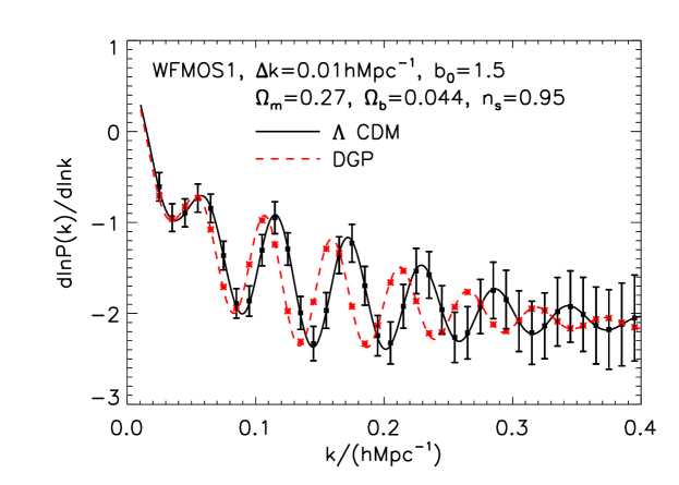
In Figure 9, we present theoretical predictions of $d\ln P/d\ln k$ for the WFMOS1 galaxy sample based on the $\Lambda$CDM (solid line) and modified DGP model (dashed line) presented in Figure 3. The data points with error bars are derived from our mock data with the wavenumber binsize of $\Delta k=0.01h{\rm Mpc}^{-1}$. We then compare the predictions of the $\Lambda$CDM model and the DGP model ($n=2$) with the mock data in Figure 9 using data points in the range $0.02<k<0.2~{}h{\rm Mpc}^{-1}$. Based on chi–square, we find that these two models are different by 6 $\sigma$. The statistical difference, with respect to the $\Lambda$CDM model, decreases to 2$\sigma$ for a modified DGP model with $n=3$, while modified gravity models with $n\geq 4$ are only statistically different at the 1$\sigma$ level. Therefore, Figure 9 demonstrates that the BAO analysis of the WFMOS1 galaxy sample will be able to discriminate between the standard $\Lambda$CDM cosmology and the original DGP models. Moreover, such analyses one will put stringent constraints on the modified DGP models with $n\geq 3$ especially when combined other independent cosmological observations.

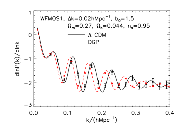
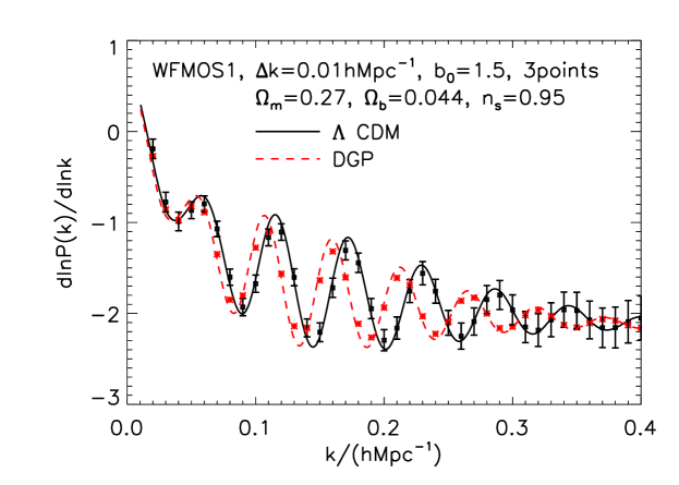
For the actual analysis of the WFMOS galaxy power spectra, the binsize ($\Delta k$) will be determined to ensure the statistical independence of adjacent bins, which will depend on the final survey geometry and the number density of observed galaxies. To test the effect of such issues on our results, we present in Figure 10 new predictions based on a binsize of $\Delta k=0.02h{\rm Mpc}^{-1}$. Furthermore, in Figure 11, we adopt the nearest three points in computing $dP/dk$ from the mock data. Taken together, Figures 10 and 11 demonstrate our results are robust against the details of binning the data. Nevertheless the statistical significance of the constraints should be carefully examined by properly taking account of the covariance matrix analysis of different data points, which is beyond the scope of the present paper.

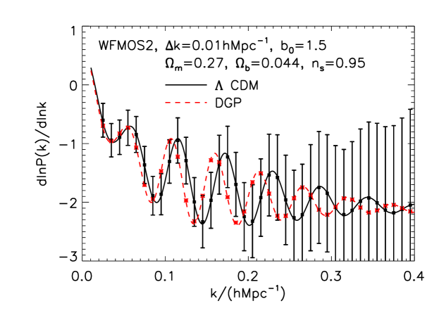
Figure 12 is similar to Figure 9 but now for the higher redshift WFMOS2 galaxy sample discussed above. The theoretical curves are almost the same as those for the WFMOS1 sample, but the error bars are now a factor 2 to 3 larger, because the theoretical curves are determined by the factors $r(z)/r^{(f)}(z)$ and $H^{(f)}(z)/H(z)$ (Figures 1 and 2) which are almost constant over the redshift range $0.5<z<3$.

To estimate future cosmological constraints, Figure 13 shows the contour of $\Delta\chi^{2}$ in the $\Omega_{m}$ and $1/n$ parameter plane for both the WFMOS1 (solid curve) and WFMOS2 (dashed curve) galaxy samples. This is similar to Figure 8 for the existing SDSS LRG sample. In this figure, the underlying cosmological model is $\Lambda$CDM with $\Omega_{m}=0.27$, $n_{s}=0.95$ and $\Omega_{b}=0.044$. Using Monte Carlo simulations, we create 100 mock datasets and computed $d\ln P(k)/d\ln k$ with a binsize of $\Delta k=0.01h{\rm Mpc}^{-1}$ (Figure 9) and then we compute the average $\Delta\chi^{2}$ statistic. The errors on the power spectrum were determined from the effective volume of the WFMOS1 and WFMOS2 samples, and the amplitude of the power spectrum (the volume of the WFMOS2 sample is assumed to be a quarter of WFMOS1 volume). Furthermore, we assumed the same bias parameter ($b_{0}=1.5$) which causes a decrease in the amplitude of power spectrum of WFMOS2 by a factor $2$.

We also consider here a new WFMOS sample of galaxies (called “WFMOS3”) which consists of $2.2\times 10^{6}$ galaxies over $1200$ deg² at $2.3<z<3.3$. This gives the same number density as the WFMOS2 sample, but with almost same volume as the WFMOS1 sample. We also assume $b_{0}=1.9$, so that the amplitude of the power spectrum is almost same as the WFMOS1 sample. We present in Figure 13 the contour of $\Delta\chi^{2}$ for the WFMOS3 sample (dotted curve), which demonstrates that such a sample would provide similar cosmological constraints as the WFMOS1 sample.

The error of $d\ln P/d\ln k$ can also be improved by increasing the mean number density of galaxies. The range of the relevant wavenumber (the maximum wavenumber) is also important for constraining the parameters. These factors will be able to improve the constraint.

Finally, we stress that our analysis is based on the fitting of $d\ln P(k)/d\ln k$. In general, however, the fitting of $P(k)$ gives more stringent constraint. Then, the constraint in this paper can be improved when using the fitting of $P(k)$ directly. But, in our analysis, we fixed the cosmological parameters $n_{s}$ and $\Omega_{b}$. Uncertainty of these factors might weaken the constraint.

VI Discussion and Conclusions

We have considered here how models of modified gravity affect the BAO signature in the power spectra of galaxy clustering both for current and future galaxy samples. As a specific model of the modified gravity, we adopt the modified DGP modelsfk which is characterized by an index $n$; the model with $n=2$ corresponds to the original DGP modelDGP , while $n=\infty$ approaches the concordance, spatially flat, $\Lambda$CDM model in general relativity. We have shown that the different expansion history in the modified gravity models shifts the peak positions of oscillations relative to the $\Lambda$CDM model. These predicted shifts in the BAO can potentially be used to distinguish between the $\Lambda$CDM model and the modified DGP model.

We tested our predictions for the BAO against existing data from the SDSS LRG sample and found we can already rule out the original DGP modified gravity model (with $n=2$) if we assume $\Omega_{m}<0.3$ with the flat geometry, although we have not carried out a full analysis of the parameter space (cf. Maartens ; SSH ). For future WFMOS galaxy samples, there is great promise for putting stringent constraints on the modified gravity.

We also note that our work is based on the linear theory of density perturbation. The non-linear nature of the gravity force in the DGP cosmology is not clear at present. It might be expected that the modification of the Poisson equation would vanish by the non-linear nature. However, this problem remains unsolved.

In our investigation, we focused on the quantity $d\ln{P}(k)/d\ln k$ in extracting the oscillation feature. As demonstrated in the last section, the theoretical curve and the result of the simulation is slightly different. This comes from the finite binsize effect, which becomes problematic when the bin of $k$ is large. This gap might be resolved by introducing a new algorithm for estimating in ${d{P}/d\ln k}$. Following the conventional method of evaluating the power spectrum with a discrete number density field FKP ; Y2003 ; YNKBN , the power spectrum can be obtained by using the estimator, adopting the constant weight factor,

$$P({\bf k})=\Bigl{[}\int d{\bf s}\bar{n}({\bf s})^{2}\Bigr{]}^{-1}\left|\sum_{i}^{N}e^{i{\bf k}\cdot{\bf s}_{i}}-{\alpha}\sum_{j}^{N/\alpha}e^{i{\bf k}\cdot{\bf s}_{j}}\right|^{2}-{\rm shot~{}noise~{}term},$$ (23)

where ${\bf s}_{i}~{}(1\leq i\leq N)$ is the $i$-th galaxy’s position of a real catalog, ${\bf s}_{j}~{}(1\leq j\leq N/\alpha)$ is the $j$-th galaxy’s position of a random catalog, and $\alpha$ a parameter chosen as $\alpha\ll 1$. In the similar way, we can evaluate the differentiation of the power spectrum by introducing the estimator

$$k{\partial P({\bf k})\over\partial k} = \Bigl{[}\int d{\bf s}\bar{n}({\bf s})^{2}\Bigr{]}^{-1}\biggl{(}\sum_{i_{1}}^{N}i{\bf k}\cdot{\bf s}_{i_{1}}e^{i{\bf k}\cdot{\bf s}_{i_{1}}}-{\alpha}\sum_{j_{1}}^{N/\alpha}i{\bf k}\cdot{\bf s}_{j_{1}}e^{i{\bf k}\cdot{\bf s}_{j_{1}}}\biggr{)}\biggl{(}\sum_{i_{2}}^{N}e^{-i{\bf k}\cdot{\bf s}_{i_{2}}}-{\alpha}\sum_{j_{2}}^{N/\alpha}e^{-i{\bf k}\cdot{\bf s}_{j_{2}}}\biggr{)}$$ (24)

$$+{\rm complex~{}conjugate}~{}.$$

This expression gives an alternative way to evaluate ${d{P}(k)/d\ln k}$. The effectiveness of the use of this estimator will be investigated as a future work.

Finally, we note the degeneracy between the DGP models used in this paper and other dark energy models. As demonstrated in Linder ; Polarski , the expansion history of the DGP model can be reproduced by a dark energy model with an effective equation of state of $w_{\rm eff}(z)\simeq w_{0}+w_{a}\times z/(1+z)$. The behavior of the galaxy power spectrum of the DGP model presented in this paper can thus be re–interpreted using this effective equation of state. This is because the WFMOS surveys only constrain the expansion history of the Universe and therefore, the measurement of the power spectrum alone can not differentiate between the DGP model and more complex dark energy models if they have the same expansion history. Observationally, weak lensing measurements can be more sensitive to the growth factor than the BAO. Therefore HyperSuprime and other large weak lensing surveys will be very useful in breaking this degeneracy while weak lensing in turn suffers from an $\Omega_{K}$ degeneracy that BAO can break bernstein . Together BAO and weak lensing offer a powerful synergy in the hunt for the origin of cosmic acceleration. We hope to return to this point in future.

Figure 1: $r(z)/r^{(f)}(z)$ as function of $z$ for the DGP model (dashed red curve), the DGP-like modified gravity models $n=4$ (dotted blue curve), $n=8$ (dash-dotted green curve), and the $\Lambda$CDM model (solid black curve). Here the density parameter is fixed as $\Omega_{m}=0.27$.

Figure 2: Same as Fig. 1 but for $H^{(f)}(z)/H(z)$. The DGP model (dashed red curve), the DGP-like modified gravity models $n=4$ (dotted blue curve), $n=8$ (dash-dotted green curve), and the $\Lambda$CDM model (solid black curve). Here $\Omega_{m}=0.27$ as Fig. 1.

Figure 3: Theoretical curves of ${d\ln{P}/d\ln k}$ for the DGP model (dashed red curve), the DGP-like modified gravity models $n=4$ (dotted blue curve), $n=8$ (dash-dotted green curve), and the $\Lambda$CDM model (solid black curve) assuming the sample WFMOS1. The modified gravity with large $n$ approaches to the $\Lambda$CDM model. Here we adopted the initial power spectral index, $n_{s}=0.95$, and $\Omega_{b}=0.044$ and $\Omega_{m}=0.27$.

Figure 4: Theoretical curves of ${d\ln{P}/d\ln k}$ in the $\Lambda$CDM model showing the effect of changing $\Omega_{m}$: the solid curve has $\Omega_{m}=0.27$, the dashed curve has $\Omega_{m}=0.22$, the dotted curve has $\Omega_{m}=0.32$. The other parameters are the same as those of Fig. 3, $n_{s}=0.95$ and $\Omega_{b}=0.044$.

Figure 5: Theoretical curves of ${d\ln{P}/d\ln k}$ in the $\Lambda$CDM model showing the effect of varying $\Omega_{b}$: the solid curve has $\Omega_{b}=0.044$, the dashed curve has $\Omega_{b}=0.04$, and the dotted curve has $\Omega_{m}=0.05$. The other parameters are the same as those of Fig. 3, $n_{s}=0.95$ and $\Omega_{m}=0.27$.

Figure 6: ${d\ln{P}/d\ln k}$ of the SDSS LRG sample and the corresponding theoretical curves of the DGP model (dashed red curves) and the $\Lambda$ CDM model (solid black curve). The thick curves are the best fit model which has $\Omega_{m}=0.32$ and $\Omega_{b}=0.045$ for the $\Lambda$ CDM model, and $\Omega_{m}=0.35$ and $\Omega_{b}=0.053$ for the DGP model. The thin dashed curve is the DGP model with the same parameter as the $\Lambda$ CDM model ($\Omega_{m}=0.32$ and $\Omega_{b}=0.045$). The other cosmological parameter $n_{s}=0.95$ is the same as in Fig. 3. The error bar is evaluated using the simple simulation with the measured power spectrum and the covariance matrix in ref. [9].

Figure 7: (a) Contour of $\Delta\chi^{2}$ on the parameter space $\Omega_{m}$ and $\Omega_{b}/\Omega_{m}$. The other parameters are fixed as the same as those in Fig. 3. The solid curve is the $\Lambda$ CDM model and the dashed curve is the DGP model. The contour level is $\Delta\chi^{2}=2.3$ (1$\sigma$; inner curve) and $\Delta\chi^{2}=6.2$ (2$\sigma$; outer curve). Here $n_{s}=0.95$ as before. (b) Same as (a) but with $h=0.66$.

Figure 8: Contour of $\Delta\chi^{2}$ on the parameter space $\Omega_{m}$ and $1/n$ in the DGP-like model. $n=2$ corresponds to the DGP model. The other parameters are fixed as $n_{s}=0.95$ and $\Omega_{b}=0.044$. The contour level is $\chi^{2}=2.3$ (1$\sigma$; inner curve) and $\chi^{2}=6.2$ (2$\sigma$; outer curve).

Figure 9: Theoretical predictions for ${d\ln{P}/d\ln k}$ assuming the sample WFMOS1 (corresponding to $z<1.3$). The squares with error bar are evaluated with the simple simulation of the power spectrum for the $\Lambda$ CDM model. The asterisks are the DGP model, but the error bar, which is almost the same as that of the $\Lambda$ CDM model, is omitted for simplicity. Theoretical curves are the DGP model (dashed red curve) and the $\Lambda$ CDM model (solid black curve). The parameters are the same as those in Fig. 3, i.e, $n_{s}=0.95$, $\Omega_{b}=0.044$, $\Omega_{m}=0.27$ and $b_{0}=1.5$. Here we used the nearest two points in the differentiation and $\Delta k=0.01~{}h{\rm Mpc}^{-1}$.

Figure 10: Same as Fig. 9, but for the case $\Delta k=0.02~{}h{\rm Mpc}^{-1}$. The parameters are chosen as $n_{s}=0.95$, $\Omega_{b}=0.044$, $\Omega_{m}=0.27$ and $b_{0}=1.5$.

Figure 11: Same as Fig. 9, but for the case of the differentiation with the nearest three points. The parameters are chosen as $n_{s}=0.95$, $\Omega_{b}=0.044$, $\Omega_{m}=0.27$ and $b_{0}=1.5$.

Figure 12: Same as Fig. 9, but for the sample WFMOS2, which assumes the range of the redshift $2.3<z<3.3$ with $\bar{n}=4\times 10^{-4}({h^{-1}\rm Mpc})^{-3}$, and a survey area $300~{}{\rm deg.}^{2}$, which yields a total number $5.5\times 10^{5}$ galaxies. The parameters are chosen as $n_{s}=0.95$, $\Omega_{b}=0.044$, $\Omega_{m}=0.27$ and $b_{0}=1.5$.

Figure 13: (a, solid curve) Contour of $\Delta\chi^{2}$ on the parameter space $\Omega_{m}$ and $1/n$ in the DGP-like model, assuming the sample WFMOS1, which consists of $2.1\times 10^{6}$ galaxies over $2000$ deg² at $0.5<z<1.3$ with the mean number density $\bar{n}=5\times 10^{-4}~{}({h^{-1}\rm Mpc})^{-3}$. The target model is the $\Lambda$ CDM model, i.e., $1/n=0$ and $\Omega_{m}=0.27$, and assumed the bias parameter $b_{0}=1.5$. Here we fixed $n_{s}=0.95$, $\Omega_{b}=0.044$. The contour level is $\chi^{2}=6.2$ (2$\sigma$). (b, dashed curve) Same as (a) but for the sample WFMOS2, which consists of $5.5\times 10^{5}$ galaxies over $300$ deg² at $2.3<z<3.3$ with the mean number density $\bar{n}=4\times 10^{-4}~{}({h^{-1}\rm Mpc})^{-3}$, and assumed the bias parameter $b_{0}=1.5$. (c, dotted curve) Same as (a) but for the sample WFMOS3, which consists of the $2.2\times 10^{6}$ galaxies over $1200$ deg² at $2.3<z<3.3$ with the mean number density $\bar{n}=4\times 10^{-4}~{}({h^{-1}\rm Mpc})^{-3}$, and assumed the bias parameter $b_{0}=1.9$.