Power-law Parameterized Quintessence Model

Abstract

We introduce a power-law parameterized quintessence model for the dark energy which accelerate universe at the low redshifts while behaves as an ordinary matter for the early universe. We construct a unique scalar potential for this parameterized quintessence model. As the observational test, the Supernova Type Ia (SNIa) Gold sample data, size of baryonic acoustic peak from Sloan Digital Sky Survey (SDSS), the position of the acoustic peak from the CMB observations and structure formation from the $2$dFGRS survey are used to constrain the parameters of the quintessence model. The best fit parameters indicates that the equation of state of this model at the present time is less than one $(w_{0}<-1)$ which violates the energy condition in General Relativity. Finally we compare the age of old objects with age of universe in this model.
PACS numbers: 95.36.+x ,98.62.Py

]

I Introduction

Observations of the apparent luminosity and redshift of type Ia supernovas (SNIa) provide the main evidence for the positive accelerating expansion of the Universe [1, 2]. A combined analysis of SNIa and the Cosmic Microwave Background radiation (CMB) observations indicates that the dark energy filled about $2/3$ of the total energy of the Universe and the remained part is dark matter with a few percent in the form of Baryonic matter from the Big Bang nucleo synthesis [3, 4, 5].

The ”cosmological constant” is a possible solution for the acceleration of the universe [6]. This constant term in Einstein field equation can be regarded as an fluid with the equation of state of $w=-1$. However, there are two problems with the cosmological constant, namely the fine-tuning and the cosmic coincidence. In the framework of quantum field theory, the vacuum expectation value is $123$ order of magnitude larger that the observed value of $10^{-47}$ GeV⁴. The absence of a fundamental mechanism which sets the cosmological constant zero or very small value is the cosmological constant problem. The second problem as the cosmic coincidence, states that why are the energy densities of dark energy and dark matter nearly equal today?

One of the solutions to this problem is a model with varying cosmological constant decays from the beginning of the universe to a small value at the present time. A non-dissipative minimally coupled scalar field, so-called Quintessence model can play the role of time varying cosmological constant [7, 8, 9]. The ratio of energy density of this field to the matter density increases slowly by the expansion of the universe and after a while the dark energy becomes the dominated term of energy-momentum tensor. One of the features of this model is the variation of equation of state during the expansion of the universe. Various Quintessence models as k-essence [10], tachyonic matter [11], Phantom [12, 13] and Chaplygin gas [14] provide various equation of states for the dark energy [13, 15, 16, 17, 18, 19, 20, 21].

There are also phenomenological models, parameterize the equation of state of dark energy in terms of redshift [22, 23, 24]. For a dark energy with the equation of state of $p_{X}=w_{X}\rho_{X}$, using the continuity equation, the density of dark energy changes with the scale factor as:

$$\rho_{X}=\rho_{X}^{(0)}a^{-3(1+\bar{w}_{X}(a))},$$ (1)

where $\bar{w}_{X}(a)$ is the mean of the equation of state in the logarithmic scale:

$$\bar{w}_{X}(a)=\frac{\int w_{X}(a)d\ln(a)}{\int{d\ln(a)}}$$ (2)

The main aim of these models is to cure the fine-tuning problem of the dark energy density by means that the ratio of dark energy density to the matter density $(\rho_{m}\sim a^{-3})$,

$$\frac{\rho_{X}}{\rho_{m}}=\frac{\rho_{X}^{(0)}}{\rho_{m}^{(0)}}a^{-3\bar{w}_{X}(a)}$$ (3)

approach to unity at the early universe in contrast to that of cosmological constant. Here we propose a simple power-law model for the mean value of equation of state as:

$$\bar{w}_{X}(a)=w_{0}a^{\alpha},$$ (4)

which can remove the fine-tuning problem of the dark energy at the early universe. This model is expressed with the two parameter of $w_{0}$ (equation of state at the present time) and the exponent of $\alpha$. The equation of state of this model according to the definition of ${\bar{w}_{X}}(a)$ obtain as:

$$w(a)=w_{0}a^{\alpha}(1+\ln{a^{\alpha}})$$ (5)

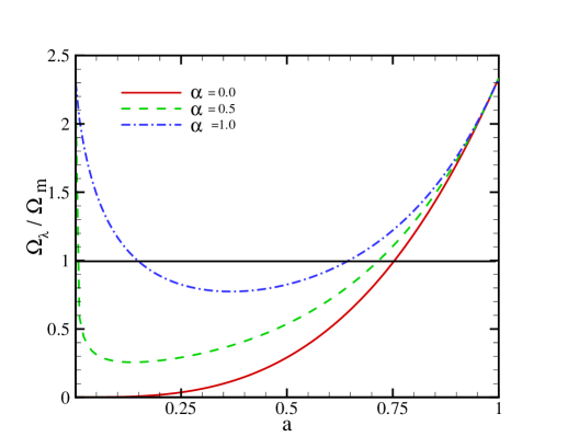
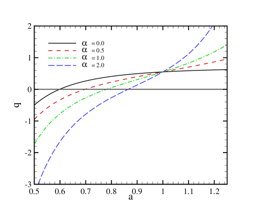
One of the advantages of this model is that for the small scale factors in the range of $a<e^{-1/\alpha}$, the sign of the equation of state will change to the positive value and the dark energy will behave as an ordinary matter. Figure (1) shows the ratio of dark energy to the matter densities as a function of scale factor for various values of $\alpha$. For $\alpha<1.3$ we have two times of domination of dark energy during the history of universe: once for the early universe and the other time at the lower red-shifts. However, since the sign of the equation of state of dark energy at the early time is positive, it will not accelerate universe and we will have only one phase of the acceleration for the later times. Figure (2) shows the deceleration parameter $(q=-\ddot{a}a/{\dot{a}^{2}})$ of the universe in terms of scale factor $a$ for various values of $\alpha$. Increasing the $\alpha$-exponent causes the universe to enter the acceleration phase of universe at the later times but speed-up it to enter the de Sitter phase faster (see Figure 2).

FIG. 1.: Ratio of dark energy to the matter density as a function of scale factor. For $0<\alpha<1.3$ we have two times of dark energy dominance over the (cold dark) matter. It should be mentioned that for the early universe the sign of equation of state will change to the positive value and behaves as a cold dark matter. Here we choose $w_{0}=-1$, $\Omega_{m}=0.3$ and $\Omega_{tot}=1.0$.

FIG. 2.: Deceleration parameter $(q=-\ddot{a}a/{\dot{a}^{2}})$ in the power-law model as a function of scale factor for various values of $\alpha$-exponent. Increasing $\alpha$ causes that universe to enter the acceleration phase at later times.

The organization of the paper is as follows: In Sec.II we reconstruct a scalar potential for generating the power-law quintessence model. In Sec.III we study the effect of this model on the age of Universe, comoving distance, comoving volume element and the variation of angular size by the redshift [25]. In Sec. IV we put constrain on the parameters of model by the background evolution, such as Gold sample of Supernova Type Ia data [26], the position of the observed acoustic angular scale on CMB and the baryonic oscillation length scale. We study the linear structure formation in this model and compare the growth index with the observations from the $2-$degree Field Galaxy Redshift Survey ($2$dFGRS) data in sec. V. We also compare the age of the universe in this model with the age of old cosmological structures in this section. Sec.VI contains summary and conclusion of this work.

II Corresponding potential of the scalar field

Scalar field is one of the physical mechanism for a time-varying dark energy that can fulfill the condition of positive acceleration of the universe at the present time. Essential condition for a given scalar field to play the role of dark energy is that the equation of state at the lower redshifts can provide the condition of $w<-1/3$. The energy density and pressure of an homogeneous scalar field with the potential of $V(\phi)$ and kinetic term of $\dot{\phi}^{2}/2$ are:

$$\rho_{X} = \frac{1}{2}\dot{\phi}^{2}+V(\phi)$$ (6)

$$P_{X} = \frac{1}{2}\dot{\phi}^{2}-V(\phi)$$ (7)

Using, the definition of equation of state of dark energy, $w_{X}=P/\rho$, the equation of state in terms of kinetic and potential energies of scalar field can be written as:

$$w_{X}=\frac{T+V}{T-V},$$ (8)

The kinetic and potential energies of scalar field from the equations (6) and (7) in terms of $\rho_{X}$ and the equation of state of dark energy are:

$$T=\frac{1}{2}\rho_{X}(1+w_{X})$$ (9)

$$V=\frac{1}{2}\rho_{X}(1-w_{X}),$$ (10)

For a positive $T$ and $V$ the equation of state is bounded to the interval $-1<w<+1$. For $T>0$ and $V<0$ we have $|w|>1$ and for the case of $T<0$ the equation of state can be $w<-1$ (i.e. kinetic term of Lagrangian has negative sign). Here we reconstruct a scalar potential which can generate the power-law quintessence model. The kinetic term of the scalar field from the equation (9) in terms of redshift obtain as [27]:

$$\frac{d\phi}{dz}=\pm\frac{[\rho_{X}(z)(1+w_{X})]^{1/2}}{H(z)(1+z)},$$ (11)

where the minus or plus sign are chosen if $\dot{\phi}>0$ and $\dot{\phi}<0$, respectively. Choosing the sign is arbitrary as it can be changed by the field redefinition of $\phi\rightarrow-\phi$. Here we choose the negative sign for convenient. The Hubble parameter also is given by:

$$H^{2}(z)=H_{0}^{2}[\Omega^{(0)}_{m}(1+z)^{3}+\Omega^{(0)}_{\lambda}(1+z)^{3[1+\bar{w}(z)]}],$$ (12)

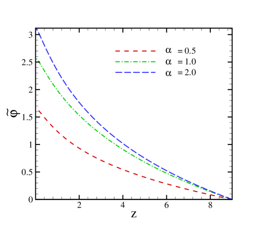
where we can substitute the Hubble parameter at the present time with $H_{0}^{2}=\rho_{c}^{(0)}/{3M_{pl}^{2}}$. Using the numerical integration we obtain the dependence of the scalar field, $\tilde{\phi}=\phi/M_{pl}$ in terms of the redshift (Figure 3). On the other hand using equation (10) we can obtain the potential in terms of redshift as:

$$\tilde{V}(z)=\frac{1}{2}(1-w_{X})F(z),$$ (13)

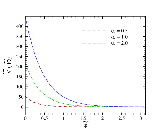
where $F(z)=\rho_{X}(z)/\rho_{X}(0)$ and $\tilde{V}(z)=V(z)/V(0)$. Finally we do numerical integration from the equation (11) and obtain the dependence of the redshift to the scalar field $z=f(\phi)$. Substituting this function in the equation (13) results the explicit relation between the potential and scalar field or in another word, reconstruction of the scalar potential for the power-law quintessence model is obtained (see Figure 4).

FIG. 3.: Dependence of scalar field in terms of redshift for the power-law Quintessence model.

FIG. 4.: Reconstruction of the scalar field potential as a function of scalar field for the power-law Quintessence model.

III the effect of variable dark energy on the geometrical parameters of universe

The cosmological observations are mainly affected by the background dynamics of universe. In this section we study the effect of the power-law dark energy model on the geometrical parameters of universe.

A comoving distance

The radial comoving distance is one of the basis parameters of cosmology. For an object with the redshift of $z$, using the null geodesics in the FRW metric, the comoving distance obtain as:

$$r(z;\alpha,w_{0})=\int_{0}^{z}{dz^{\prime}\over H(z^{\prime};\alpha,w_{0})},$$ (14)

where $H(z;\alpha,w_{0})$ is the Hubble parameter and after the matter-radiation equality epoch, it can be expressed in terms of Hubble parameter at the present time, $H_{0}$, matter and dark energy content of the universe.

FIG. 5.: Comoving distance, $r(z;\alpha,w_{0})$ (in unit of $c/H_{0}$) as a function of redshift for various values of $\alpha$. Here we fix $w_{0}=-1$.

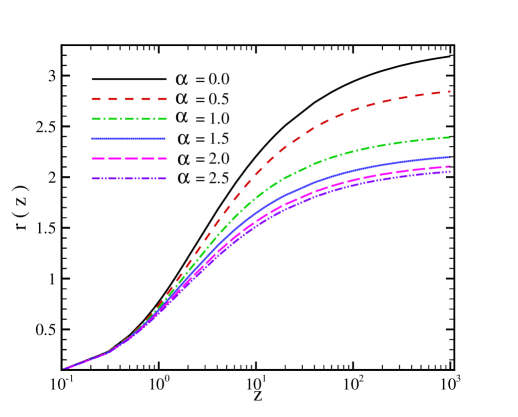
By numerical integration of equation (14), the comoving distance in terms of redshift for different values of $\alpha$ is shown in Figure 5. Increasing the $\alpha$ exponent, increases the contribution of dark energy at the present time and results a smaller comoving distance. One of the main applications of the comoving distance calculation is on the analyzing of luminosity distance of SNIa data.

B Angular Size

Measurement of apparent angular size of an object located at the cosmological distance is another important parameter that can be affected by the amount and variation of dark energy during the history of universe. An object with the physical size of $D$ is related to the apparent angular size of $\theta$ by:

$$D=d_{A}\theta$$ (15)

where $d_{A}=r(z;\alpha,w_{0})/(1+z)$ is the angular diameter distance. The main applications of equation (15) is on the measurement of the apparent angular size of acoustic peak on CMB and baryonic acoustic peak at the lower redshifts. By measuring the angular size of an object in different redshifts (so-called Alcock-Paczynski test) it is possible to probe the variability of dark energy [25]. The variation of apparent angular size $\Delta\theta$ in terms $\Delta z$ is given by:

$${\Delta z\over\Delta\theta}=\frac{H(z;\alpha,w_{0})r(z;\alpha,w_{0})}{\theta}$$ (16)

FIG. 6.: Alcock-Paczynski test, compares $\Delta z/{\Delta\theta}$ normalized to the case of $\Lambda$CDM model as a function of redshift for four different $\alpha$.

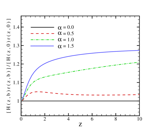
Figure 6 shows $\Delta z/\Delta\theta$ in terms of redshift, normalized to the case with $\alpha=0$ (i.e. $\Lambda$CDM model). The advantage of Alcock-Paczynski test is that it is independent of standard candles and a standard ruler such as the size of baryonic acoustic peak can be used to constrain the dark energy model.

C Comoving Volume Element

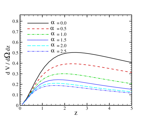
The comoving volume element is an other geometrical parameter which is used in number-count tests such as lensed quasars, galaxies, or clusters of galaxies. The comoving volume element in terms of comoving distance and Hubble parameters is given by:

$$f(z;\alpha,w_{0})\equiv{dV\over dzd\Omega}=r^{2}(z;\alpha,w_{0})/H(z;\alpha,w_{0}).$$ (17)

According to Figure 7, the comoving volume element becomes maximum around $z\simeq 2$. For a larger $\alpha$ exponent, the position of the peak of comoving volume element shifts to the lower redshifts.

FIG. 7.: The comoving volume element in terms of redshift for various $\alpha$ exponent. Increasing $\alpha$ shifts the position of maximum value of volume element to the lower redshifts.

D Age of Universe

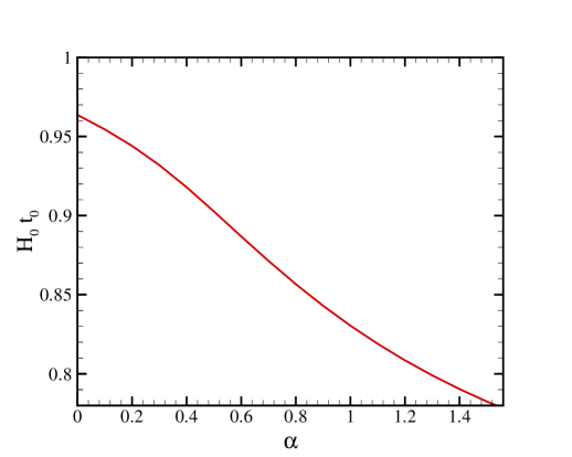
The ”age crises” is one the main reasons for the existence of dark energy. The problem is that the universe’s age in the Cold Dark Matter (CDM) universe is less than the age of old stars in it. Studies on the old stars [28] suggests an age of $13^{+4}_{-2}$ Gyr for the universe. Richer et. al. [29] and Hasen et. al. [30] also proposed an age of $12.7\pm 0.7$ Gyr, using the white dwarf cooling sequence method (for full review of the cosmic age see [5]). The age of universe integrating from the big bang up to now obtain as:

$$t_{0}(\alpha,w_{0})=\int_{0}^{t_{0}}\,dt=\int_{0}^{\infty}{dz\over(1+z)H(z;\alpha,w_{0})},$$ (18)

Figure 8 shows the dependence of $H_{0}t_{0}$ (Hubble parameters times the age of universe) on $\alpha$-exponent for a typical values of cosmological parameters (e.g. $h=0.65$, $\Omega_{m}=0.27$ and $w_{0}=-1.0$). Increasing $\alpha$ results a shorter age for the universe.

FIG. 8.: $H_{0}t_{0}$ (age of universe times the Hubble constant at the present time) as a function of $\alpha$ in a flat universe with the parameters of $\Omega_{m}=0.3$, $h=0.65$ and $w_{0}=-1.0$. Increasing $\alpha$-exponent makes a shorter age for the universe.

IV Observational Constraint From the Background Evolution

In this section we compare the SNIa Gold sample data, the location of baryonic acoustic peak from the SDSS and the location of acoustic peak from the CMB observation to constrain the parameters of model.

A Examining Model by Supernova Type Ia: Gold Sample

The Supernova Type Ia experiments provided the main evidence of the existence of dark energy. Since 1995 two teams of the High-Z Supernova Search and the Supernova Cosmology Project have been discovered several type Ia supernovas at the high redshifts [17, 31]. Recently Riess et al.  (2004) announced the discovery of $16$ type Ia supernova with the Hubble Space Telescope. This new sample includes $6$ of the $7$ most distant ($z>1.25$) type Ia supernovas. They determined the luminosity distance of these supernovas and with the previously reported algorithms, obtained a uniform $157$ Gold sample of type Ia supernovas [26, 32, 33].

In this subsection we compare the predictions of the dark energy model with the SNIa Gold sample. The observations of supernova measure essentially the apparent magnitude $m$ including reddening, K correction etc, which is related to the (dimensionless) luminosity distance, $D_{L}$, of a an object at redshift $z$, for a spatially flat universe by:

$$m={\mathcal{M}}+5\log{D_{L}(z;\alpha,w_{0})},$$ (19)

where

$$D_{L}(z;\alpha,w_{0}) = H_{0}(1+z)\int^{z}_{0}{d\zeta\over H(\zeta;\alpha,w_{0})}\,.$$ (20)

Also

$$\mathcal{M} = M+5\log{\left(\frac{c/H_{0}}{1\quad Mpc}\right)}+25.$$ (21)

where $M$ is the absolute magnitude. The distance modulus, $\mu$, is defined as:

$$\mu\equiv m-M=5\log{D_{L}(z;\alpha,w_{0})}+5\log{\left(\frac{c/H_{0}}{1\quad Mpc}\right)}+25,$$ (22)

In order to compare the theoretical results with the observational data, we must compute the distance modulus, as given by Eq. (22). The first step in this sense is to compute the quality of the fitting through the least squared fitting quantity $\chi^{2}$ defined by:

$$\chi^{2}=\sum_{i}\frac{[\mu_{obs}(z_{i})-\mu_{th}(z_{i};\Omega_{m},w_{0},\alpha,h)]^{2}}{\sigma_{i}^{2}},$$ (23)

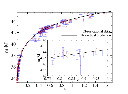
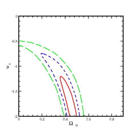
where $\sigma_{i}$ is the observational uncertainty in the distance modulus. To constrain the parameters of model, we use the Likelihood statistical analysis Marginalizing over the nuisance parameter of $h$ in a flat universe $(\Omega_{total}=1)$, the best fit values for the parameters of model obtain as $w_{0}=-2.60_{-2.00}^{+1.80}$, $\Omega_{m}=0.45^{+0.09}_{-0.45}$ and $\alpha=1.00_{-1.00}^{+1.00}$ with $\chi^{2}_{min}/N_{d.o.f}=1.13$ at $1\sigma$ level of confidence. The corresponding value for the Hubble parameter at the minimized $\chi^{2}$ is $h=0.66$ and since we have already marginalized over this parameter we do not assign an error bar for it. Figure 9 shows the best fit of model to the Gold sample of SNIa. We compare our result with that of Riess et al. (2004), for $\alpha=0$ their result has been recovered (see Figure 10).

For the age consistency test we substitute the parameters of model from the SNIa fitting in equation (18) and obtain the age of universe about $13.19$ Gry, which is in good agreement with the age of old stars.

FIG. 9.: Fitting the distance modulus of the SNIa Gold sample in terms of redshift with the power-law dark energy model. Solid line shows the best fit with the corresponding parameters of $h=0.66$, $w_{0}=-2.60_{-2.00}^{+1.80}$, $\Omega_{m}^{=}0.45^{+0.09}_{-0.45}$ and $\alpha=1.00_{+1.00}^{-1.00}$ in $1\sigma$ level of confidence with $\chi^{2}_{min}/N_{d.o.f}=1.13$

FIG. 10.: Joint confidence intervals for $\Omega_{m}$ and $w_{0}$ for the case of $\alpha=0$ with $1\sigma$ (solid-line), $2\sigma$ (dashed-line) and $3\sigma$ (long dashed-line) confidence level. This result is in good agreement with that of Riess et al. (2004).

B Combined analysis: SNIa$+$CMB$+$SDSS

In this section we combine SNIa Gold sample, CMB data from the WMAP with recently observed baryonic peak from the SDSS to constrain the parameters of power-law dark energy model [34].

The apparent acoustic peak is the most relevant parameter in the spectrum of CMB which can be used to determine the geometry and the matter content of universe. The acoustic peak corresponds to the Jeans length of photon-baryon structures at the last scattering surface some $\sim 379$ Kyr after the Big Bang [5]. The apparent angular size of acoustic peak in a flat universe can be obtained by dividing the comoving size of sound horizon at the decoupling epoch $r_{s}(z_{dec})$ to the comoving distance of observer to the last scattering surface $r(z_{dec})$:

$$\theta_{A}\equiv{{r_{s}(z_{dec})}\over r(z_{dec})}.$$ (24)

The size of sound horizon at numerator of equation (24) corresponds to the a distance that a perturbation of pressure can travel from the beginning of universe up to the last scattering surface and obtain by:

$$r_{s}(z_{dec};\alpha,w_{0})=\int_{z_{dec}}^{\infty}\frac{v_{s}(z)}{H(z;\alpha,w_{0})}dz,$$ (25)

where $v_{s}(z)^{-2}=3+9/4\times\rho_{b}(z)/\rho_{r}(z)$ is the sound velocity in the unit of speed of light from the big bang up to the last scattering surface [19, 35].

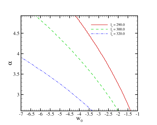
Changing the parameters of the dark energy can change the size of apparent acoustic peak and subsequently the position of $l_{A}\equiv\pi/\theta_{A}$ in the power spectrum of temperature fluctuations on CMB. Here we plot the dependence of $l_{A}$ on $\alpha$ and $w_{0}$ for a typical values of cosmological parameters (see Figure 11).

FIG. 11.: Dependence of acoustic angular scale $l_{A}$ on $\alpha$ and $w_{0}$ for the three cases of $l_{A}=290$ (solid-line), $300$ (dashed-line) and $320$ (dashed-dotted line).

In order to compare the observed angular size of acoustic peak with that of model, we use the shift parameter $R$ as [36]:

$$R=\sqrt{\Omega_{m}}\int_{0}^{z_{dec}}\frac{dz}{E(z;\alpha,w_{0})},$$ (26)

where $E(z;\alpha,w_{0})=H(z;\alpha,w_{0})/H_{0}$. The shift parameter is proportional to the size of acoustic peak to that of flat pure-CDM, $\Lambda=0$ model, ($R\propto\theta_{A}/\theta_{A}^{\it flat}$). The observational result of CMB experiments correspond a shift parameter of $R=1.716\pm 0.062$ (given by WMAP, CBI, ACBAR) [5, 37]. One of the advantages of using the parameter $R$ is that it is independent of Hubble constant.

Recently detected size of baryonic peak in the SDSS is the third observational data for our analysis. The correlation function of 46,748 Luminous Red Galaxies (LRG) from the SDSS shows a well detected baryonic peak around $100$ Mpc $h^{-1}$. This peak has an excellent match to the predicted shape and the location of the imprint of the recombination-epoch acoustic oscillation on the low-redshift clustering matter [38]. For a flat universe we can construct the parameter $A$ as follows:

$$A=\sqrt{\Omega_{m}}E(z_{1};\alpha,w_{0})^{-1/3}\times\left[\frac{1}{z_{1}}\int_{0}^{z_{1}}\frac{dz}{E(z;\alpha,w_{0})}\right]^{2/3}.$$ (27)

We use the robust constraint on the dark energy model using the value of $A=0.469\pm 0.017$ from the LRG observation at $z_{1}=0.35$ [38].

In what follows we perform a combined analysis of SNIa, CMB and SDSS to constrain the parameters of dark energy model by minimizing the combined $\chi^{2}=\chi^{2}_{\rm{SNIa}}+\chi^{2}_{{\rm CMB}}+\chi^{2}_{{\rm SDSS}}$. The best values of the model parameters from the fitting with the corresponding error bars from the likelihood function marginalizing over the Hubble parameter in the multidimensional parameter space results: $\Omega_{m}=0.32_{-0.04}^{+0.03}$, $\alpha=1.60_{-0.90}^{+0.60}$ and $w_{0}=-2.00_{-0.40}^{+0.80}$ at $1\sigma$ confidence level with $\chi^{2}_{min}/N_{d.o.f}=1.13$. The Hubble parameter corresponds to the minimum value of $\chi^{2}$ is $h=0.66$. Here we obtain an age of $12.82$ Gyr for the universe. Table I indicates the best fit values for the cosmological parameters with one and two $\sigma$ level of confidence.

TABLE I.: The best values for the parameters of power-law dark energy model with the corresponding age for the universe from the fitting with the SNIa, SNIa+CMB+SDSS and SNIa+CMB+SDSS+LSS experiments at one and two $\sigma$ confidence level.

Observation	$\Omega_{m}$	$\alpha$	$w_{0}$	age (Gyr)
	$0.45^{+0.09}_{-0.45}$	$1.00^{+1.00}_{-1.00}$	$-2.60^{+1.80}_{-2.00}$
SNIa				$13.19$
	$0.45^{+0.13}_{-0.45}$	$1.00^{+2.00}_{-1.00}$	$-2.60^{+1.90}_{-2.90}$
SNIa+CMB	$0.32^{+0.03}_{-0.04}$	$1.60^{+0.60}_{-0.90}$	$-2.00^{+0.80}_{-0.40}$	$12.82$
+SDSS
	$0.32^{+0.05}_{-0.08}$	$1.60^{+1.40}_{-1.60}$	$-2.00^{+1.30}_{-1.30}$
SNIa+CMB	$0.31^{+0.02}_{-0.04}$	$0.80^{+0.70}_{-0.30}$	$-1.40^{+0.40}_{-0.65}$	$13.72$
SDSS+LSS
	$0.31^{+0.04}_{-0.06}$	$0.80^{+1.60}_{-0.80}$	$-1.40^{+0.60}_{-1.10}$

V Constraints by Large Scale structure

So far we have only considered observations related to the background evolution. In this section using the linear approximation of structure formation we obtain the growth index of structures and compare it with result of observations by the $2$-degree Field Galaxy Redshift Survey ($2$dFGRS).

The continuity and Poisson equations for the density contrast $\delta=\delta\rho/\bar{\rho}$ in the cosmic fluid provides the evolution of density contrast in the linear approximation (i.e. $\delta\ll 1$)[39, 40] as:

$$\ddot{\delta}+2\frac{\dot{a}}{a}\dot{\delta}-\left({v_{s}}^{2}\nabla^{2}+4\pi G\rho\right)\delta=0,$$ (28)

where the dot denotes the derivative with respect to time. The effect of dark energy in the evolution of the structures in this equation enters through its influence on the expansion rate. Here we assume that dark energy distributed uniformly as the background fluid and it doesn’t contribute in clustering of matter. The validity of this linear Newtonian approach is restricted to perturbations on the sub-horizon scales but large enough where structure formation is still in the linear regime [39, 40]. For the perturbations larger than the Jeans length, $\lambda_{J}=\pi^{1/2}v_{s}/\sqrt{G\rho}$, equation (28) for cold dark matter (CDM) reduces to:

$$\ddot{\delta}+2\frac{\dot{a}}{a}\dot{\delta}-4\pi G\rho\delta=0$$ (29)

The equation for the evolution of density contrast can be re-written in terms of scale factor as:

$$\frac{d^{2}\delta}{da^{2}}+\frac{d\delta}{da}\left[\frac{\ddot{a}}{\dot{a}^{2}}+\frac{2H}{\dot{a}}\right]-\frac{3H_{0}^{2}}{2\dot{a}^{2}a^{3}}\Omega_{m}\delta=0$$ (30)

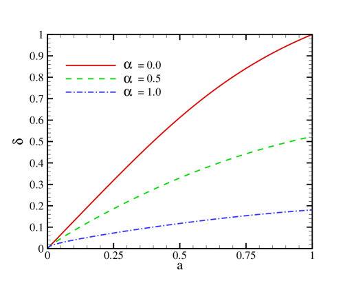
where the dot denotes the time derivative. Numerical solution of equation (30) in a FRW universe in the background of power-law dark energy model is shown in Figure 12. In the CDM model, the density contrast $\delta$ grows linearly with the scale factor, while we have a deviation from the linearity as soon as dark energy begins to dominate. As larger $\alpha$ is, universe enters the dark energy domination earlier (see Figure 1) which results in a lesser growth of the density contrast.

FIG. 12.: Evolution of density contrast as a function of scale factor for different values of $\alpha$ exponent in the flat universe with $\Omega_{m}=0.3$, $\Omega_{\lambda}=0.7$ and $w_{0}=-1.0$.

In the linear perturbation theory, the peculiar velocity field $\bf{v}$ is determined by the density contrast [39, 41] as:

$${\bf v}({\bf x})=H_{0}\frac{f}{4\pi}\int\delta({\bf y})\frac{{\bf x}-{\bf y}}{\left|{\bf x}-{\bf y}\right|^{3}}d^{3}{\bf y},$$ (31)

where the growth index $f$ is defined by:

$$f=\frac{d\ln\delta}{d\ln a},$$ (32)

and it is proportional to the ratio of the second term of equation (29) (friction) by the third (Poisson) term.

We use the evolution of the density contrast $\delta$ to compute the growth index of structure $f$, which is an important quantity for the interpretation of peculiar velocities of galaxies, as discussed in [41, 42] for the Newtonian and the relativistic regime of structure formation. Replacing the density contrast with the growth index in equation(30) results the evolution of growth index as:

$$\frac{df}{d\ln a}=\frac{3H_{0}^{2}}{2a^{3}}\Omega_{m}-f^{2}$$ (33)

$$- f\left[2-\frac{H_{0}^{2}}{2}[\frac{2}{H_{0}^{2}}+\frac{\Omega_{m}}{a^{3}}+\Omega_{\Lambda}(a)(1+3w(a))]\right]$$ (34)

Figure 13 shows the numerical solution of (33) in terms of redshift.

FIG. 13.: Growth index versus redshift for different values of $\alpha$. Here we take a typical values for the cosmological parameters of $\Omega_{m}=0.3$ and $\Omega_{\lambda}=0.7$ and $w_{0}=-1.0$.

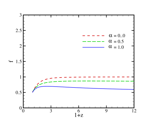
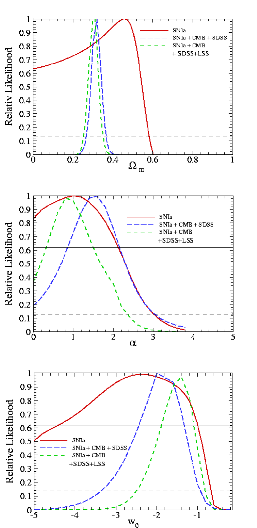
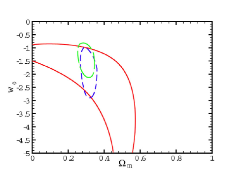
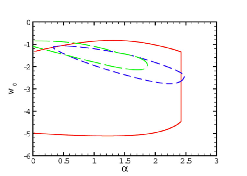
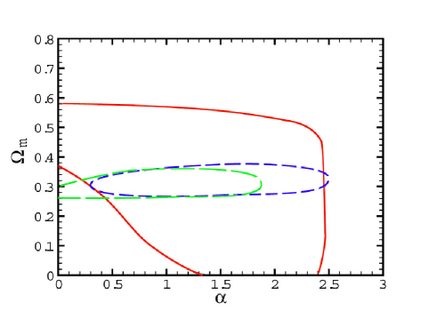
The observation of $220,000$ galaxies with the $2$dFGRS experiment provides the numerical value of growth index [38]. By measurements of two-point correlation function, the $2$dFGRS team reported the redshift distortion parameter of $\beta=f/b=0.49\pm 0.09$ at $z=0.15$, where $b$ is the bias parameter describes the difference in the distribution of galaxies and mass. Verde et al. (2003) used the bispectrum of $2$dFGRS galaxies [43, 44] and obtained $b_{verde}=1.04\pm 0.11$ which resulted $f=0.51\pm 0.10$. Now we fit the growth index at the present time derived from the equation (33) with the observational value. This fitting gives a loss constraint to the parameters of the model, so in order to have a better confinement of the parameters, we combine this fitting with those of SNIa$+$CMB$+$SDSS which has been discussed at the last section. We perform the least square fitting by minimizing $\chi^{2}=\chi_{\rm{SNIa}}^{2}+\chi_{\rm{CMB}}^{2}+\chi_{\rm{SDSS}}^{2}+\chi_{\rm{LSS}}^{2}$. The best fit values with the corresponding error bars for the model parameters are: $\Omega_{m}=0.31^{+0.02}_{-0.04}$, $\alpha=0.80_{-0.30}^{+0.70}$ and $w_{0}=-1.40_{-0.65}^{+0.40}$ at $1\sigma$ confidence level with $\chi^{2}_{min}/N_{d.o.f}=1.15$. The error bars have been obtain through the likelihood functions $(\mathcal{L}$$\propto e^{-\chi^{2}/2})$ marginalizing over the nuisance parameter of $h$ [45]. The Hubble parameter corresponds to the minimum value of $\chi^{2}$ is $h=0.65$. The likelihood functions for the three cases of (i) fitting model with Supernova data, (ii) combined analysis with the three experiments of SNIa$+$CMB$+$SDSS and (iii) combining all four experiments of SNIa$+$CMB$+$SDSS$+$LSS are shown in Figure 14. The joint confidence contours in the $(\Omega_{m},w_{0})$, $(\alpha,\Omega_{m})$ and $(w_{0},\alpha)$ planes also are shown in Figures 15, 16 and 17.

Finally we do the consistency test, comparing the age of universe derived from this model with the age of old stars and Old High Redshift Galaxies (OHRG) in various redshifts. Table I shows that the age of universe from the combined analysis of SNIa$+$CMB$+$SDSS$+$LSS is $13.72$ Gyr which is in agreement with the age of old stars [28]. Here we take three OHRG for comparison with the power-law dark energy model, namely the LBDS $53$W$091$, a $3.5$-Gyr old radio galaxy at $z=1.55$ [46], the LBDS $53$W$069$ a $4.0$-Gyr old radio galaxy at $z=1.43$ [47] and a quasar, APM $08279+5255$ at $z=3.91$ with an age of $t=2.1_{-0.1}^{+0.9}$Gyr [48]. The later one has once again led to the ”age crisis”. An interesting point about this quasar is that it cannot be accommodated in the $\Lambda$CDM model [49]. To quantify the age-consistency test we introduce the expression $\tau$ as:

$$\tau=\frac{t(z;\alpha,w_{0})}{t_{obs}}=\frac{t(z;\alpha,w_{0})H_{0}}{t_{obs}H_{0}},$$ (35)

where $t(z)$ is the age of universe, obtain from the equation (18) and $t_{obs}$ is an estimation for the age of old cosmological object. In order to have a compatible age for the universe we should have $\tau>1$. Table II shows the value of $\tau$ for three mentioned OHRG. We see that the parameters of dark energy model from the SNIa and CMB observations don’t provide a compatible age for the universe, compare to the age of old objects, while combination with the LSS data results a longer age for the universe. Once again for the power-law dark energy model, APM $08279+5255$ at $z=3.91$ has longer age than the universe.

TABLE II.: The value of $\tau$ for three high redshift objects, using the parameters of the model derived from the fitting with the observations.

Observation	LBDS $53$W$069$	LBDS $53$W$091$	APM
			$08279+5255$
	$z=1.43$	$z=1.55$	$z=3.91$
SNIa	$0.92$	$0.97$	$0.59$
SNIa+CMB	$0.83$	$0.88$	$0.50$
+SDSS
SNIa+CMB	$1.01$	$1.07$	$0.65$
+SDSS+LSS

FIG. 14.: Marginalized likelihood functions of three parameters of dark energy model ($\Omega_{M}$, $\alpha$ and $w_{0}$). The solid line corresponds to the likelihood function of fitting the model with SNIa data, the long dashed-line with the joint SNIa$+$CMB$+$SDSS data and dashed-line corresponds to SNIa$+$CMB$+$SDSS$+$LSS. The intersections of the curves with the horizontal solid and dashed lines give the bounds with $1\sigma$ and $2\sigma$ level of confidence respectively.

FIG. 15.: Joint confidence intervals of $\Omega_{m}$ and $w_{0}$, fitting with SNIa (solid line), SNIa$+$CMB$+$SDSS (dashed-line) and SNIa$+$CMB$+$SDSS$+$LSS (long dashed-line) with $1\sigma$ level of confidence.

FIG. 16.: Joint confidence intervals of $\alpha$ and $w_{0}$, fitting with the SNIa (solid line), SNIa$+$CMB$+$SDSS (dashed-line) and SNIa$+$CMB$+$SDSS$+$LSS (long dashed-line) with $1\sigma$ level of confidence.

FIG. 17.: Joint confidence intervals of $\Omega_{m}$ and $\alpha$, fitting with the SNIa (solid line), SNIa$+$CMB$+$SDSS (dashed-line) and SNIa$+$CMB$+$SDSS$+$LSS (long dashed-line) with $1\sigma$ level of confidence.

VI conclusion

We proposed a power-law parameterized quintessence model with the mean-equation of state of $\bar{w}(z)=w_{0}a^{\alpha}$. An exponential potential of scalar field is proposed for generating this type of dark energy model. The effect of this model on the age of universe, radial comoving distance, comoving volume element and the variation of apparent size of objects with the redshift (Alcock-Paczynski test) have been studied. In order to constrain the parameters of model we fit our model with the Gold sample SNIa data, CMB shift parameter, location of baryonic acoustic peak observed by SDSS and large scale structure data by $2$dFGRS. The best parameters from the fitting obtained as: $h=0.65$, $\Omega_{m}=0.31^{+0.02}_{-0.04}$, $\alpha=0.80_{-0.30}^{+0.70}$ and $w_{0}=-1.40_{-0.65}^{+0.40}$ at $1\sigma$ confidence level with $\chi^{2}_{min}/N_{d.o.f}=1.15$. The best fit for the equation of state at the present time provides that $w_{0}<-1$, which violates the strong energy condition in general relativity. Furthermore for $w_{0}<-1$ the kinetic term of scalar field in the Lagrangian is negative [50, 51] (theoretical attempts for $w<-1$ can be found at  [52, 53, 54, 55, 56, 57]).

We also did the age test, comparing the age of old stars and old high redshift galaxies with the age derived from the power-law dark energy model. From the best fit parameters of the model we obtained an age of $13.72$ Gyr for the universe which is in agreement with the age of old stars. We also chose two high redshift radio galaxies at $z=1.55$ and $z=1.43$ with a quasar at $z=3.91$. The two first objects were consistent with the age of universe by means that there were younger than the age of universe while the later one was older than the age of universe.

REFERENCES

- [1] A. G. Riess et al., Astron. J. 116, 1009 (1998).
- [2] S. Perlmutter et al., Astrophys. J. 517, 565 (1999).
- [3] C. L. Bennett et al., Astrophys. J. Suppl. Ser. 148, 1 (2003).
- [4] H.V. Peiris et al., Astrophys. J. Suppl. Ser. 148, 213 (2003).
- [5] D. N. Spergel, L. Verde, H. V. Peiris et al., Astrophys. J. 148, 175 (2003).
- [6] S. Weinberg, Rev. Mod. Phys. 61, 1 (1989; S. M. Carroll, Living Rev. Relativity 4, 1 (2001); P. J. E. Peebles and B. Ratra, Rev. Mod. Phys. 75, 559 (2003); T. Padmanabhan, Phys. Rep. 380, 235 (2003).
- [7] C. Wetterich, Nucl. Phys. B302, 668 (1988); P. J. E. Peebles and B. Ratra, Astrophys. J. 325, L17 (1988); B. Ratra and P. J. E. Peebles, Phys. Rev. D 37, 3406 (1988); J. A. Frieman, C. T. Hill, A. Stebbins, and I. Waga, Phys. Rev. Lett. 75, 2077 (1995); M. S. Turner and M. White, Phys. Rev. D 56, R4439 (1997); R. R. Caldwell, R. Dave, and P. J. Steinhardt, Phys. Rev. Lett. 80, 1582 (1998); A. R. Liddle and R. J. Scherrer, Phys. Rev. D 59, 023509 (1999); I. Zlatev, L.Wang, and P. J. Steinhardt, Phys. Rev. Lett. 82, 896 (1999); P. J. Steinhardt, L. Wang, and I. Zlatev, Phys. Rev. D 59, 123504 (1999); D. F. Torres, Phys. Rev. D 66, 043522 (2002).
- [8] L. Amendola, Phys. Rev. D 62, 043511 (2000); L. Amendola and D. Tocchini-Valentini, Phys. Rev. D 64, 043509 (2001); 66, 043528 (2002); L. Amendola, Mon. Not. R. Astron. Soc. 342, 221 (2003); M. Pietroni, Phys. Rev. D 67, 103523 (2003); D. Comelli, M. Pietroni, and A. Riotto, Phys. Lett. B 571, 115 (2003); U. Franca and R. Rosenfeld, Phys. Rev. D 69, 063517 (2004); X. Zhang, astro-ph/0503072; Phys. Lett. B 611, 1 (2005).
- [9] P. J. E. Peebles, R. Ratra, Astrophys. J. 325, L17 (1988).
- [10] C. Armendariz-Picon, V. Mukhanov and P. J. Steinhardt, Phys. Rev. Lett. 85, 4438 (2000).
- [11] J. S. Bagla, H. K. Jassal and T. Padmanabhan, Phys. Rev. D 67, 063504 (2003).
- [12] R. R. Caldwell, Phys. Lett. B 545, 23 (2002).
- [13] R. R. Caldwell, M. Kamionkowski and N. N. Weinberg, Phys. Rev. Lett. 91, 071301 (2003).
- [14] A. Kamenshchik, U. Moschella and V. Pasquier, Phys. Lett. B 511, 265 (2001).
- [15] S. Arbabi-Bidgoli, M. S. Movahed and S. Rahvar, astro-ph/0508323.
- [16] L. Wang, R. R. Caldwell, J. P. Ostriker and P. J. Steinhardt, Astrophys. J. 530, 17 (2000).
- [17] S. Perlmutter, M. S. Turner and M. White, Phys. Rev. Lett. 83, 670 (1999).
- [18] L. Page et al., Astrophys. Supp. J. 148, 233 (2003).
- [19] M. Doran, M. Lilley,J. Schwindt and C. Wetterich, Astrophys. J. 559, 501 (2001).
- [20] M. Doran, M. Lilley, Mon. Not.Roy. A. Soc. 330, 965 (2002).
- [21] R. R. Caldwell and M. Doran, Phys. Rev. D 69, 103517 (2004).
- [22] M. Chevallier, D. Polarski and A. Starobinsky, Int. J. Mod. Phys D 10, 213 (2001).
- [23] E. V. Linder, Phys. Rev. Lett. 90, 091301 (2003).
- [24] U. Seljak et al., Phys. Rev. D 71, 103515 (2005).
- [25] C. Alcock and B. Paczynski, Nature 281, 358 (1979).
- [26] A. G. Riess et al., Astrophys. J. 607, 665 (2004).
- [27] Zong-Kuan Guo, Nobuyoshi Ohta and Yuan-Zhong Zhang, Phys. Rev. D 72, 023504 (2005).
- [28] E. Carretta et al., Astrophys. J. 533, 215 (2000); L. M. Krauss and B. Chaboyer, astro-ph/0111597; B. Chaboyer and L. M. Krauss, Astrophys. J. Lett. 567, L45 (2002).
- [29] H. B. Richer et al., Astrophys. J. 574, L151 (2002).
- [30] B. M. S. Hansen et al., Astrophys. J. 574, L155 (2002).
- [31] B. P. Schmidt et al., Astrophys. J. 507, 46 (1998).
- [32] J. L. Tonry et al., Astrophys. J. 594, 1 (2003).
- [33] B. J. Barris et al., Astrophys. J. 602, 571 (2004).
- [34] C. L. Bennett, R. S, Hill and G. Hinshaw, Astrophys. J. Suppl. 148, 97 (2003).
- [35] W. Hu and N. Sugiyama, Astrophys. J. 444, 489 (1995).
- [36] J. R. Bond, G. Efstathiou, and M. Tegmark, Mon. Not. R. Astron. Soc. 291, L33 (1997); A. Melchiorri, L. Mersini, C. J. Odman, and M. Trodden, Phys. Rev. D 68, 043509 (2003); C. J. Odman, A. Melchiorri, M. P. Hobson, and A. N. Lasenby, Phys. Rev. D 67, 083511 (2003).
- [37] T. J. Pearson et al. (CBI Collaboration), Astrophys. J. 591, 556 (2003); C. L. Kuo et al. (ACBAR Collaboration), Astrophys. J. 600, 32 (2004).
- [38] D. J. Eisenstein et al., astro-ph/0501171.
- [39] Padmanabhan T., 1993, Structure Formation in the Universe. Cambridge Univ. Press
- [40] Brandenberger, R. H., 2004, in Breton N., Cervantes-Cota J. L., and Salgado, M., eds, Lecture Notes in Physics, , The early universe and observational cosmology, 646, p.127
- [41] Peebles, P. J. E., 1980, The Large Scale Structure of the Universe, Princeton University Press, Princeton, NJ
- [42] Mansouri, R., Rahvar, S, 2002, IJMPD, 11, 312
- [43] Verde L., Kamionkowski M., Mohr J. J., Benson A.J., 2001, MNRAS, 321, L7
- [44] Lahav O., Bridle S. L., Percival W. J., & the 2dFGRS Team, 2002, MNRAS, 333, 961
- [45] W. H. Press, S. A. Teukolsky, W. T. Vettering and B. P. Flannery, Numerical Recipes, Cambridge University Press, Cambridge, 1994.
- [46] J. Dunlop et. al., Nature (London) 381, 581 (1996); H. Spinrard, Astrophys. J. 484, 581 (1997).
- [47] J. Dunlop, in The Most Distant Radio Galaxies, edited by H. J. A. Rottgering, P. Best, and M. D. Lehnert (Kluwer, Dordrecht, 1999), p. 71.
- [48] G. Hasinger, N. Schartel and S. Komossa, Astrophys. J. Lett. 573, L77 (2002); S. Komossa and G. Hasinger, astro-ph/0207321.
- [49] D. Jain., A. Dev., astro-ph/0509212 (accepted in Phys. Lett. B)
- [50] S. M. Carroll, M. Hoffman and M. Trodden, Phys. Rev. D 68, 023509 (2003).
- [51] S. W. Hawking, G.F.R. Ellis, The Large Scale Structure of Space-Time, Cambridge University Press, Cambridge (1973).
- [52] R. R. Caldwell, Phys. Lett. B 545, 23 (2002) [arXiv:astro-ph/9908168].
- [53] A. E. Schulz and M. J. White, Phys. Rev. D 64, 043514 (2001) [arXiv:astro-ph/0104112].
- [54] L. Parker and A. Raval, Phys. Rev. D60, 063512 (1999)
- [55] P.H. Frampton, astro-ph/0209037.
- [56] M. Ahmed, S. Dodelson, P. B. Greene and R. Sorkin, arXiv:astro-ph/0209274.
- [57] S. M. Carroll, M. Hoffman and M. Trodden, arXiv:astro-ph/0301273.