Perturbation Theory Reloaded: Analytical Calculation of Non-linearity in Baryonic Oscillations in the Real Space Matter Power Spectrum

Abstract

We compare the non-linear matter power spectrum in real space calculated analytically from 3rd-order perturbation theory with $N$-body simulations at $1<z<6$. We find that the perturbation theory prediction agrees with the simulations to better than 1% accuracy in the weakly non-linear regime where the dimensionless power spectrum, $\Delta^{2}(k)=k^{3}P(k)/2\pi^{2}$, which approximately gives variance of matter density field at a given $k$, is less than 0.4. While the baryonic acoustic oscillation features are preserved in the weakly non-linear regime at $z>1$, the shape of oscillations is distorted from the linear theory prediction. Nevertheless, our results suggest that one can correct the distortion caused by non-linearity almost exactly. We also find that perturbation theory, which does not contain any free parameters, provides a significantly better fit to the simulations than the conventional approaches based on empirical fitting functions to simulations. The future work would include perturbation theory calculations of non-linearity in redshift space distortion and halo biasing in the weakly non-linear regime.

1. Introduction

Cosmological linear perturbation theory has been remarkably successful in explaining the precision measurements of temperature and polarization anisotropies of the cosmic microwave background (CMB), most notably from the Wilkinson Microwave Anisotropy Probe (WMAP) Bennett et al. (2003). The CMB data, combined with linear theory, have enabled us to determine many of the cosmological parameters to better than 10% accuracy Spergel et al. (2006). As the CMB data improve, however, it has become increasingly clear that one has to combine the CMB data with the other probes to break degeneracies between the parameters that cannot be constrained very well by the CMB data alone. For example, the CMB alone cannot break degeneracy between the equation of state of dark energy, $w$, and matter density, $\Omega_{m}$ Spergel et al. (2006).

The large-scale structure (LSS) of the universe has also been known as an excellent probe of cosmological fluctuations as well as cosmological parameters, as proven successfully by the Two-degree Field Galaxy Redshift Survey (2dFGRS) Cole et al. (2005) and the Sloan Digital Sky Survey (SDSS) Tegmark et al. (2004); Seljak et al. (2005). A joint analysis of the future CMB and LSS data is extremely powerful in constraining most of the cosmological parameters to better than a few percent accuracy (e.g., Takada et al., 2006). In particular, the LSS data would allow us to constrain “additional” parameters such as the mass of neutrinos and the shape of the primordial power spectrum, which would remain relatively poorly constrained by the CMB data alone.

The success of this approach depends on our ability to predict the power spectrum of CMB and LSS from theory. Linear theory provides adequate precision for CMB, as the amplitude of CMB anisotropy is only $10^{-5}$; however, theory of LSS has not reached to the point where one can use LSS for precision cosmology at the level similar to CMB. There is a larger degree of non-linearity in LSS. In order for the LSS data to be as powerful as the CMB data, it is crucial that we can predict the LSS power spectrum to 1% accuracy, which is nearly one order of magnitude better than the current precision.

In principle, theory of LSS may be developed using $N$-body simulations. This approach has been widely used in the literature. One method builds on the so-called HKLM formalism Hamilton et al. (1991), which interpolates between the linear regime on large scales and the stable clustering regime on small scales using a fitting function to $N$-body simulations. The HKLM method was further elaborated by Peacock & Dodds (1996). The other method builds on the so-called halo model Scherrer & Bertschinger (1991), which was further elaborated by e.g., Seljak (2000); Smith et al. (2003). Both approaches are based on empirical methods, fitting to $N$-body simulations mainly at $z\sim 0$. While these predictions may be good to within 10%, one should not expect 1% accuracy from these. Also, these methods, in their current form, do not allow for non-linearity in redshift space distortion in the weakly non-linear regime, which limits their practical use for the actual data analysis.

We use an alternative approach based on cosmological perturbation theory (PT). One can calculate the next-to-leading order correction to the linear power spectrum by using 3rd-order PT Vishniac (1983); Suto & Sasaki (1991); Makino et al. (1992); Jain & Bertschinger (1994); Scoccimarro & Frieman (1996). The advantage of PT is that it provides an exact solution for the non-linear matter power spectrum as long as one applies it to the region in $k$ space where perturbative expansion is valid. (We shall call this region in $k$ space the “weakly non-linear regime”.) One still needs to use simulations to find the maximum $k$ below which perturbation expansion is valid, which is one of the goals of this paper.

Cosmological PT, including non-linear corrections to the power spectrum, was actively investigated in 1990’s (Bernardeau et al., 2002, for a review). In particular, a lot of efforts have been devoted into understanding the non-linear power spectrum at $z\sim 0$. It was shown that perturbation approach would not provide accurate descriptions of the power spectrum at $z\sim 0$ due to too strong non-linearity. Our results are consistent with the previous work; however, we focus on the power spectrum at $z>1$, where non-linearity is still modest and thus PT should perform better.

Our work is motivated by recent proposals of high-$z$ galaxy survey projects such as the Cosmic Inflation Probe (CIP) Melnick et al. (2005), Hobby-Ebery Dark Energy Experiment (HETDEX) Hill et al. (2004), and Wide-field Fiber-fed Multi Object Spectrograph (WFMOS) survey Glazebrook et al. (2005), to mention a few. The goal of these missions is to measure the power spectrum of high-$z$ galaxies to a few percent accuracy. These missions should be able to measure the baryonic features in the power spectrum accurately. On the other hand, it has been pointed out that non-linearity would distort the baryonic features in a complex way so that it might be challenging to extract the underlying baryonic features from the observed galaxy power spectrum Meiksin et al. (1999); Springel et al. (2005); White (2005); Seo & Eisenstein (2005). We show that, as far as non-linearity in the matter power spectrum in real space is concerned, we can correct it almost exactly.

This paper is organized as follows. We briefly review the 3rd-order PT in § 2, and describe our $N$-body numerical simulations in § 3. We compare the analytical predictions with simulations in § 4. We pay a particular attention to non-linearity in the baryonic acoustic oscillations. We give discussion and conclusions in § 5. We test convergence of our results in Appendix A.

2. Non-linear Matter Power spectrum: 3rd-order Perturbation Theory

We review 3rd-order PT calculations of the next-to-leading order correction to the matter power spectrum, following the pioneering work in the literature Vishniac (1983); Fry (1984); Goroff et al. (1986); Suto & Sasaki (1991); Makino et al. (1992); Jain & Bertschinger (1994); Scoccimarro & Frieman (1996). As the power spectrum, $P(k,\tau)$, is a quadratic quantity of the density field in Fourier space, $\tilde{\delta}_{\mathbf{k}}(\tau)$,

$$\langle\tilde{\delta}_{\mathbf{k}}(\tau)\tilde{\delta}^{*}_{{\mathbf{k}}^{\prime}}(\tau)\rangle=(2\pi)^{3}P(k,\tau)\delta_{D}({\mathbf{k}}-{\mathbf{k}}^{\prime}),$$ (1)

the 3rd-order expansion in the density field is necessary for obtaining the next-to-leading order correction to $P(k,\tau)$. We often use the “dimensionless power spectrum”, $\Delta^{2}(k,\tau)$, which represents the contribution to the variance of density field per $\ln k$,

$$\langle\delta^{2}({\mathbf{x}},\tau)\rangle=\int\frac{dk}{k}~{}\Delta^{2}(k,\tau),$$ (2)

where $\Delta^{2}(k,\tau)\equiv k^{3}P(k,\tau)/(2\pi^{2})$.

We treat dark matter and baryons as pressureless dust particles, as we are interested in the scales much larger than the Jeans length. We also assume that peculiar velocity is much smaller than the speed of light, which is always an excellent approximation, and that the fluctuations we are interested in are deep inside the horizon; thus, we treat the system as Newtonian. The basic equations to solve are given by

$$\dot{\delta}+\nabla\cdot[(1+\delta)\mathbf{v}]=0,$$ (3)

$$\dot{\mathbf{v}}+(\mathbf{v}\cdot\nabla)\mathbf{v}=-\frac{\dot{a}}{a}\mathbf{v}-\nabla\phi,$$ (4)

$$\nabla^{2}\phi=4\pi Ga^{2}\bar{\rho}\delta,$$ (5)

where the dots denote $\partial/\partial\tau$ ($\tau$ is the conformal time), $\nabla$ denotes $\partial/\partial{\mathbf{x}}$ (${\mathbf{x}}$ is the comoving coordinate), ${\mathbf{v}}=d{\mathbf{x}}/d\tau$ is the peculiar velocity field, and $\phi$ is the peculiar gravitational potential field from density fluctuations. We assume that ${\mathbf{v}}$ is curl-free, which motivates our using $\theta\equiv\nabla\cdot\mathbf{v}$, the velocity divergence field. Using equation (5) and the Friedmann equation, we write the continuity equation [Eq. (3)] and the Euler equation [Eq. (4)] in Fourier space as

$$\dot{\tilde{\delta}}_{\mathbf{k}}(\tau)+\tilde{\theta}_{\mathbf{k}}(\tau)$$

$$= -\int\frac{d^{3}k_{1}}{(2\pi)^{3}}\int d^{3}k_{2}\delta_{D}(\mathbf{k}_{1}+\mathbf{k}_{2}-\mathbf{k})\frac{\mathbf{k}\cdot\mathbf{k}_{1}}{k^{2}_{1}}\tilde{\delta}_{{\mathbf{k}}_{2}}(\tau)\tilde{\theta}_{{\mathbf{k}}_{1}}(\tau),$$

$$\dot{\tilde{\theta}}_{\mathbf{k}}(\tau)+\frac{\dot{a}}{a}\tilde{\theta}_{\mathbf{k}}(\tau)+\frac{3\dot{a}^{2}}{2a^{2}}\Omega_{\rm m}(\tau)\tilde{\delta}_{\mathbf{k}}(\tau)$$

$$= -\int\frac{d^{3}k_{1}}{(2\pi)^{3}}\int d^{3}k_{2}\delta_{D}(\mathbf{k}_{1}+\mathbf{k}_{2}-\mathbf{k})\frac{k^{2}(\mathbf{k}_{1}\cdot\mathbf{k}_{2})}{2k_{1}^{2}k_{2}^{2}}\tilde{\theta}_{{\mathbf{k}}_{1}}(\tau)\tilde{\theta}_{{\mathbf{k}}_{2}}(\tau),$$

respectively.

To proceed further, we assume that the universe is matter dominated, $\Omega_{\rm m}(\tau)=1$ and $a(\tau)\propto\tau^{2}$. Of course, this assumption cannot be fully justified, as dark energy dominates the universe at low $z$. Nevertheless, it has been shown that the next-to-leading order correction to $P(k)$ is extremely insensitive to the underlying cosmology, if one uses the correct growth factor for $\tilde{\delta}_{\mathbf{k}}(\tau)$ Bernardeau et al. (2002). Moreover, as we are primarily interested in $z\geq 1$, where the universe is still matter dominated, accuracy of our approximation is even better. (We quantify the error due to this approximation below.) To solve these coupled equations, we shall expand $\tilde{\delta}_{\mathbf{k}}(\tau)$ and $\tilde{\theta}_{\mathbf{k}}(\tau)$ perturbatively using the $n$-th power of linear solution, $\delta_{1}(\mathbf{k})$, as a basis:

$$\tilde{\delta}(\mathbf{k},\tau) = \sum_{n=1}^{\infty}a^{n}(\tau)\int\frac{d^{3}q_{1}}{(2\pi)^{3}}\cdots\frac{d^{3}q_{n-1}}{(2\pi)^{3}}$$ (8)

$$\times\int d^{3}q_{n}\delta_{D}(\sum_{i=1}^{n}\mathbf{q}_{i}-\mathbf{k})$$

$$\times F_{n}(\mathbf{q}_{1},\mathbf{q}_{2},\cdots,\mathbf{q}_{n})\delta_{1}(\mathbf{q}_{1})\cdots\delta_{1}(\mathbf{q}_{n}),$$

$$\tilde{\theta}(\mathbf{k},\tau) = -\sum_{n=1}^{\infty}\dot{a}(\tau)a^{n-1}(\tau)\int\frac{d^{3}q_{1}}{(2\pi)^{3}}\cdots\frac{d^{3}q_{n-1}}{(2\pi)^{3}}$$ (9)

$$\times\int d^{3}q_{n}\delta_{D}(\sum_{i=1}^{n}\mathbf{q}_{i}-\mathbf{k})$$

$$\times G_{n}(\mathbf{q}_{1},\mathbf{q}_{2},\cdots,\mathbf{q}_{n})\delta_{1}(\mathbf{q}_{1})\cdots\delta_{1}(\mathbf{q}_{n}).$$

Here, the functions $F$ and $G$ as well as their recursion relations are given in Jain & Bertschinger (1994). As the linear density field, $\delta_{1}$, is a Gaussian random field, the ensemble average of odd powers of $\delta_{1}$ vanishes. Therefore, the next-to-leading order correction to $P(k)$ is

$$P(k,\tau)=a^{2}(\tau)P_{11}(k)+a^{4}(\tau)[2P_{13}(k)+P_{22}(k)],$$ (10)

where

$$P_{22}(k)=2\int\frac{d^{3}q}{(2\pi)^{3}}P_{11}(q)P_{11}(|\mathbf{k}-\mathbf{q}|)\left[F_{2}^{(s)}(\mathbf{q},\mathbf{k}-\mathbf{q})\right]^{2},$$ (11)

$$F_{2}^{(s)}(\mathbf{k}_{1},\mathbf{k}_{2})=\frac{5}{7}+\frac{2}{7}\frac{(\mathbf{k}_{1}\cdot\mathbf{k}_{2})^{2}}{k_{1}^{2}k_{2}^{2}}+\frac{\mathbf{k}_{1}\cdot\mathbf{k}_{2}}{2}\left(\frac{1}{k_{1}^{2}}+\frac{1}{k_{2}^{2}}\right),$$ (12)

$$2P_{13}(k) = \frac{2\pi k^{2}}{252}P_{11}(k)\int_{0}^{\infty}\frac{dq}{(2\pi)^{3}}P_{11}(q)$$ (13)

$$\times \Biggl{[}100\frac{q^{2}}{k^{2}}-158+12\frac{k^{2}}{q^{2}}-42\frac{q^{4}}{k^{4}}$$

$$+ \frac{3}{k^{5}q^{3}}(q^{2}-k^{2})^{3}(2k^{2}+7q^{2})\ln\left(\frac{k+q}{|k-q|}\right)\Biggl{]}.$$

While $F_{2}^{(s)}({\mathbf{k}}_{1},{\mathbf{k}}_{2})$ should be modified for different cosmological models, the difference vanishes when ${\mathbf{k}}_{1}\parallel{\mathbf{k}}_{2}$. The biggest correction comes from the configurations with ${\mathbf{k}}_{1}\perp{\mathbf{k}}_{2}$, for which $[F_{2}^{(s)}(\Lambda{\rm CDM})/F_{2}^{(s)}({\rm EdS})]^{2}\simeq 1.006$ and $\lesssim 1.001$ at $z=0$ and $z\geq 1$, respectively. Here, $F_{2}^{(s)}({\rm EdS})$ is given by equation (12), while $F_{2}^{(s)}(\Lambda{\rm CDM})$ contains corrections due to $\Omega_{\rm m}\neq 1$ and $\Omega_{\Lambda}\neq 0$ Matsubara (1995); Scoccimarro et al. (1998), and we used $\Omega_{\rm m}=0.27$ and $\Omega_{\Lambda}=0.73$ at present. The information about different background cosmology is thus almost entirely encoded in the linear growth factor. We extend the results obtained above to arbitrary cosmological models by simply replacing $a(\tau)$ in equation (10) with an appropriate linear growth factor, $D(z)$,

$$P(k,z)=D^{2}(z)P_{11}(k)+D^{4}(z)[2P_{13}(k)+P_{22}(k)].$$ (14)

We shall use equation (11)–(14) to compute $P(k,z)$.

3. $N$-body simulations and analysis method

We use the TVD (Ryu et al., 1993) code to simulate the evolution of $\delta({\mathbf{x}},\tau)$. The TVD code uses the Particle-Mesh scheme for gravity, and the Total-Variation-Diminishing (TVD) scheme for hydrodynamics, although we do not use hydrodynamics in our calculations. To increase the dynamic range of the derived power spectrum and check for convergence of the results, we use four box sizes, $L_{\rm box}=512$, 256, 128, and 64 $h^{-1}$ Mpc, with the same number of particles, $N=256^{3}$. (We use $512^{3}$ meshes for doing FFT.) We use the following cosmological parameters: $\Omega_{\rm m}=0.27$, $\Omega_{\rm b}=0.043$, $\Omega_{\Lambda}=0.73$, $h=0.7$, $\sigma_{8}=0.8$, and $n_{\rm s}=1$. We output the simulation data at $z=6$, 5, 4, 3, 2 and 1 for 512, 256 and 128 $h^{-1}$ Mpc, while only at $z=6$, 5, 4 and 3 for 64 $h^{-1}$ Mpc.

We suppress sampling variance of the estimated $P(k,z)$ by averaging $P(k,z)$ from 60, 60, 20, and 15 independent realizations of 512, 256, 128, and 64 $h^{-1}$ Mpc simulations, respectively. We calculate the density field on $512^{3}$ mesh points from the particle distribution by the Cloud-In-Cell (CIC) mass distribution scheme. We then Fourier transform the density field and average $|\delta_{\mathbf{k}}(\tau)|^{2}$ within $k-\Delta k/2\leq|{\mathbf{k}}|<k+\Delta k/2$ over the angle to estimate $P(k,z)$. Here, $\Delta k=2\pi/L_{\rm box}$. Finally, we correct the estimated $P(k)$ for loss of power due to the CIC pixelization effect using the window function calculated from 100 realizations of random particle distributions.

Figure 1.— Power spectrum at $z=1$, 2, 3, 4, 5 and 6 (from top to bottom), derived from $N$-body simulations (dashed lines), perturbation theory (solid lines), and linear theory (dot-dashed lines). We plot the simulation data from 512, 256, 128, and 64 $h^{-1}$ Mpc simulations at $k\leq 0.24~{}h~{}{\rm Mpc}^{-1}$, $0.24<k\leq 0.5~{}h~{}{\rm Mpc}^{-1}$, $0.5<k\leq 1.4~{}h~{}{\rm Mpc}^{-1}$, and $1.4<k\leq 5~{}h~{}{\rm Mpc}^{-1}$, respectively. Note that we did not run 64 $h^{-1}$ Mpc simulations at $z=1$ or 2.

We use the COSMICS package Bertschinger (1995) to calculate the linear transfer function (with linger) and generate the input linear matter power spectrum and initial conditions (with grafic). We have increased the number of sampling points for the transfer function in $k$ space from the default value of COSMICS, as the default sampling rate is too low to sample the baryonic acoustic oscillations accurately. (The default rate resulted in an artificial numerical smoothing of the oscillations.) We locate initial particles on the regular grid (i.e., we do not randomize the initial particle distribution), and give each particle the initial velocity field using the Zel’dovich approximation. This procedure suppresses shot noise in the derived power spectrum, which arises from randomness of particle distribution. We have checked this by comparing $P(k,z)$ from the initial condition to the input linear spectrum. However, some shot noise would arise as density fluctuations grow over time. While it is difficult to calculate the magnitude of shot noise from the structure formation, we estimate it by comparing $P(k,z)$ from large-box simulations with that from small-box simulations. We do not find any evidence for shot noise at $z\geq 1$; thus, we do not subtract shot noise from the estimated $P(k,z)$. To be conservative, we use 512, 256, 128, and 64 $h^{-1}$ Mpc simulations to obtain $P(k,z)$ at $k\leq 0.24~{}h~{}{\rm Mpc}^{-1}$, $0.24<k\leq 0.5~{}h~{}{\rm Mpc}^{-1}$, $0.5<k\leq 1.4~{}h~{}{\rm Mpc}^{-1}$, and $1.4<k\leq 5~{}h~{}{\rm Mpc}^{-1}$, respectively, to avoid the residual CIC pixelization effect and potential contaminations from unaccounted shot noise terms as well as artificial “transients” from initial conditions generated by the Zel’dovich approximation Crocce et al. (2006). The initial redshifts are $z_{\rm initial}=27$, 34, 42, and 50 for 512, 256, 128, and 64 $h^{-1}$ Mpc simulations, respectively. In Appendix A we show more on the convergence test (see Fig. 5).

4. Results

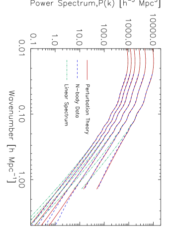
Figure 1 compares $P(k,z)$ at $z=1$, 2, 3, 4, 5 and 6 (from top to bottom) from simulations (dashed lines), PT (solid lines), and linear theory (dot-dashed lines). The PT predictions agree with simulations so well that it is actually difficult to see the difference between PT and simulations in Figure 1. The simulations are significantly above the linear theory predictions at high $k$.

Figure 2.— (Top) Dimensionless power spectrum, $\Delta^{2}(k)$. The solid and dashed lines show perturbation theory calculations and $N$-body simulations, respectively. The dotted lines show the predictions from halo approach Smith et al. (2003). The dot-dashed lines show the linear power spectrum. (Bottom) Residuals. The errorbars show the $N$-body data divided by the perturbation theory predictions minus one, while the solid curves show the halo model calculations given in Smith et al. (2003) divided by the perturbation theory predictions minus one. The perturbation theory predictions agree with simulations to better than 1% accuracy for $\Delta^{2}(k)\lesssim 0.4$.

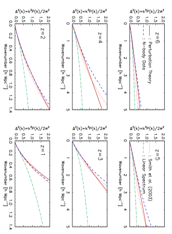
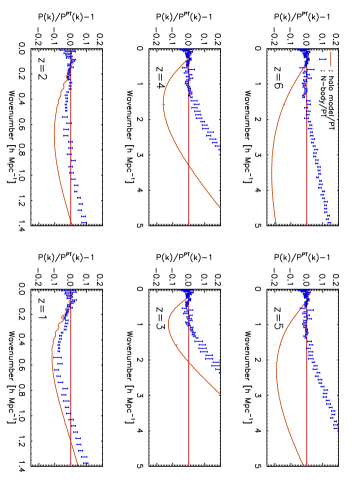
To facilitate the comparison better, we show $\Delta^{2}(k,z)$ [Eq. (2)] in Figure 2. We find that the PT predictions (thin solid lines) agree with simulations (thick solid lines) to better than 1% accuracy for $\Delta^{2}(k,z)\lesssim 0.4$. On the other hand, the latest predictions from halo approach Smith et al. (2003) (dotted lines) perform significantly worse then PT. This result suggests that one must use PT to model non-linearity in the weakly non-linear regime.

Figure 3.— Non-linearity in baryonic acoustic oscillations. All of the power spectra have been divided by a smooth power spectrum without baryonic oscillations from equation (29) of Eisenstein & Hu (1998). The errorbars show $N$-body simulations, while the solid lines show perturbation theory calculations. The dot-dashed lines show the linear theory predictions. Perturbation theory describes non-linear distortion on baryonic oscillations very accurately at $z>1$. Note that different redshift bins are not independent, as they have grown from the same initial conditions. The $N$-body data at $k<0.24$ and $k>0.24~{}h~{}{\rm Mpc}^{-1}$ are from 512 and 256 $h^{-1}$ Mpc box simulations, respectively.

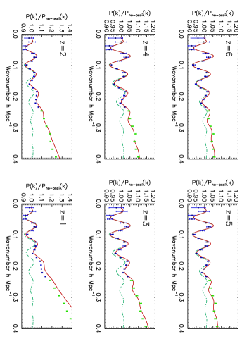
The baryonic features in the matter power spectrum provide a powerful tool to constrain the equation of state of dark energy. This method uses the fact that the CMB angular power spectrum sets the physical acoustic scale, and thus the features in the matter power spectrum seen on the sky and in redshift space may be used as the standard ruler, giving us the angular diameter distance out to the galaxy distribution at a given survey redshift as well as $H(z)$ Matsubara & Szalay (2003); Hu & Haiman (2003); Seo & Eisenstein (2003); Blake & Glazebrook (2003). In order for this method to be viable, however, it is crucial to understand distortion on the baryonic acoustic oscillations caused by non-linearity. This has been investigated so far mostly using direct numerical simulations Meiksin et al. (1999); Springel et al. (2005); White (2005); Seo & Eisenstein (2005). Meiksin et al. (1999) also compared the PT prediction with their $N$-body simulations at $z=0$, finding that PT was a poor fit. This is because non-linearity at $z=0$ is too strong to model by PT. Figure 3 shows that PT provides an accurate analytical account of non-linear distortion at $z>1$: even at $z=1$, the third peak at $k\simeq 0.18~{}h~{}{\rm Mpc}^{-1}$ is modeled at a few percent level. At $z>2$, all the oscillatory features are modeled to better than 1% accuracy. A slight deficit in power from $N$-body simulations at $k\sim 0.2~{}h~{}{\rm Mpc}^{-1}$ relative to the perturbation theory predictions at $z=2$ may be due to artificial transient modes from the Zel’dovich approximation used to generate initial conditions. One may eliminate such an effect by either using a smaller box-size or a better initial condition from the second-order Lagrangian perturbation theory Crocce et al. (2006). As the power spectrum at $k>0.24~{}h~{}{\rm Mpc}^{-1}$ from 256 $h^{-1}$ Mpc simulations at $z=2$ agrees with the perturbation theory predictions very well, we conclude that this small deficit in power at $k\sim 0.2~{}h~{}{\rm Mpc}^{-1}$ is a numerical effect, most likely the transients in low-resolution simulations.

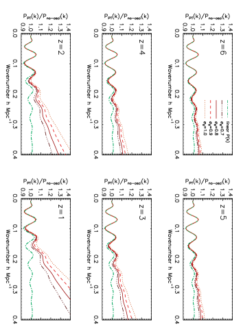
How do the predicted non-linear power spectra depend on the amplitude of matter fluctuations? As the non-linear contributions to the power spectrum are given by the linear spectrum squared, a non-linear to linear ratio grows in proportion to $\sigma_{8}^{2}$. In Fig 4 we show how the non-linear contributions increase as one increases $\sigma_{8}$ from 0.7 to 1.0. This figure may be useful when one compares our results with the previous work that uses different values of $\sigma_{8}$.

Figure 4.— Non-linearity and the amplitude of matter fluctuations, $\sigma_{8}$. In each panel the lines show the linear spectrum and non-linear spectrum with $\sigma_{8}=0.7$, 0.8, 0.9 and 1.0 from bottom to top.

5. Discussion and Conclusions

The next-to-leading order correction to the matter power spectrum calculated analytically from 3rd-order PT provides an almost exact description of the matter power spectrum in real space in the weakly non-linear regime, where $\Delta^{2}(k)\lesssim 0.4$ (Fig. 2). The most important implications of our results for the planned high-$z$ galaxy surveys are that we can use PT to calculate (a) non-linearity in the baryonic acoustic oscillations (Fig. 3), which should reduce systematics in constraining dark energy properties, and (b) the matter power spectrum up to much higher $k$ than that was accessible before, which should vastly increase our ability to measure the shape of the primordial power spectrum as well as the mass of neutrinos Takada et al. (2006). Of course, these surveys measure the galaxy power spectrum in redshift space; thus, the future work should include PT calculations of non-linearity in (a) redshift space distortion Scoccimarro (2004), and (b) halo biasing Fry & Gaztanaga (1993); Heavens et al. (1998), as well as an extensive comparison with numerical simulations. PT also allows one to calculate the higher-order statistics such as the bispectrum, which has been shown to be a powerful tool to check for systematics in our understanding of non-linear galaxy bias Matarrese et al. (1997); Verde et al. (1998). We should therefore “reload” cosmological perturbation theory and make a serious assessment of its validity in light of the planned high-$z$ galaxy surveys constraining properties of dark energy, inflation, and neutrinos.

We would like to thank D. Ryu for letting us use his TVD code, and K. Gebhardt, Y. Suto and M. Takada for comments. D.J. would like to thank K. Ahn for his help on the TVD code. E.K. acknowledges support from an Alfred P. Sloan Fellowship. The simulations were carried out at the Texas Advanced Computing Center (TACC).

Appendix A Convergence Test

To test convergence of the power spectra derived from simulations and determine the valid range in wavenumber from each simulation box, we have run $N$-body simulations with four different box sizes, $L_{\rm box}=512$, 256, 128, and 64 $h^{-1}$ Mpc, with the same number of particles, $N=256^{3}$. The initial redshifts are $z_{\rm initial}=27$, 34, 42, and 50 for 512, 256, 128, and 64 $h^{-1}$ Mpc simulations, respectively.

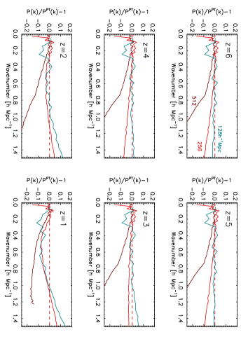
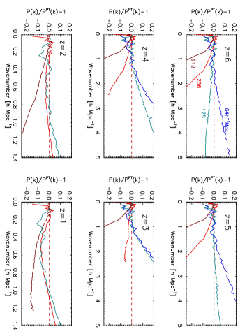
Figure 5 shows that simulations with a larger box size lack power on larger scales due to the lack of resolution, as expected, while they have better statistics on large scales than those with a smaller box size. This figure helps us to determine the valid range in wavenumber from each simulation box. We find that one can use 512, 256, 128, and 64 $h^{-1}$ Mpc simulations to calculate reliable estimates of the power spectrum in $k\leq 0.24~{}h~{}{\rm Mpc}^{-1}$, $0.24<k\leq 0.5~{}h~{}{\rm Mpc}^{-1}$, $0.5<k\leq 1.4~{}h~{}{\rm Mpc}^{-1}$, and $1.4<k\leq 5~{}h~{}{\rm Mpc}^{-1}$, respectively.

Figure 5.— Convergence test. (Left) Fractional differences between the power spectra from $N$-body simulations in $L_{\rm box}=512$, 256, and 128 $h^{-1}$ Mpc box (from bottom to top lines) and the perturbation theory predictions in $k<1.5~{}h~{}{\rm Mpc}^{-1}$. (Right) The same as left panel, but for simulations in $L_{\rm box}=512$, 256, 128, and 64 $h^{-1}$ Mpc box (from bottom to top lines) in the expanded range in wavenumber, $k<5~{}h~{}{\rm Mpc}^{-1}$.

References

- Bennett et al. (2003) Bennett, C., et al. 2003, ApJS, 148, 1
- Bernardeau et al. (2002) Bernardeau, F., Colombi, S., Gaztanaga, E., & Scoccimarro, R. 2002, Phys. Rept., 367, 1
- Bertschinger (1995) Bertschinger, E. 1995, unpublished (astor-ph/9506070)
- Blake & Glazebrook (2003) Blake, C., & Glazebrook, K. 2003, ApJ, 594, 665
- Cole et al. (2005) Cole, S., et al. 2005, MNRAS, 362, 505
- Crocce et al. (2006) Crocce, M., Pueblas, S., & Scoccimarro, R. 2006, astro-ph/0606505
- Eisenstein & Hu (1998) Eisenstein, D. J., & Hu, W. 1998, ApJ, 496, 605
- Fry (1984) Fry, J. N. 1984, ApJ, 279, 499
- Fry & Gaztanaga (1993) Fry, J. N., & Gaztanaga, E. 1993, ApJ, 413, 447
- Goroff et al. (1986) Goroff, M., Grinstein, B., Rey, S.-J., & Wise, M. 1986, ApJ, 311,6
- Glazebrook et al. (2005) Glazebrook, K., et al. 2005, A white paper submitted to the Dark Energy Task Force (astro-ph/0507457)
- Hamilton et al. (1991) Hamilton, A. J. S., Kumar, P., Edward, L., & Matthews, A. 1991, ApJ, 374, L1
- Heavens et al. (1998) Heavens, A. F., Matarrese, S., & Verde, L. 1998, MNRAS, 301, 797
- Hill et al. (2004) Hill, G. J., Gebhardt, K., Komatsu, E., & MacQueen, P. J. 2004, AIP Conf. Proc., 743, 224
- Hu & Haiman (2003) Hu, W., & Haiman, Z. 2003, PRD, 68, 063004
- Jain & Bertschinger (1994) Jain, B. & Bertschinger, E. 1994, ApJ, 431, 495
- Matarrese et al. (1997) Matarrese, S., Verde, L., & Heavens, A. F. 1997, MNRAS, 290, 651
- Meiksin et al. (1999) Meiksin, A., White, M., & Peacock, J. A. 1999, MNRAS, 304, 851
- Makino et al. (1992) Makino, N., Sasaki, M., & Suto, Y. 1992, PRD, 46, 2
- Matsubara (1995) Matsubara, T. 1995, Prog. Theor. Phys., 94, 1151
- Matsubara & Szalay (2003) Matsubara, T., & Szalay, A. 2003, PRL, 90, 021302
- Melnick et al. (2005) Melnick, G. J., et al. 2005, The NASA Origins Probe Misson Study Report, “The Cosmic Inflation Probe: Study Report”. See also http://cfa-www.harvard.edu/cip.
- Peacock & Dodds (1996) Peacock, J. A., & Dodds, S. J. 1996, MNRAS, 280, L19
- Ryu et al. (1993) Ryu, D., Ostriker, J. P., Kang, H., & Cen, R. 1993, ApJ, 414, 1
- Scherrer & Bertschinger (1991) Scherrer, R. J., & Bertschinger, E. 1991, ApJ, 381, 349
- Scoccimarro (2004) Scoccimarro, R. 2004, PRD, 70, 083007
- Scoccimarro & Frieman (1996) Scoccimarro, R., & Frieman, J. 1996, ApJ, 473, 620
- Scoccimarro et al. (1998) Scoccimarro, R., Colombi, S., Fry, J. N., Frieman, J. A., Hivon, E., & Melott, A. 1998, ApJ, 496, 586
- Seljak (2000) Seljak, U. 2000, MNRAS, 318, 203
- Seo & Eisenstein (2003) Seo, H.-J., & Eisenstein, D. 2003, ApJ, 598, 720
- Seo & Eisenstein (2005) Seo, H.-J., & Eisenstein, D. 2005, ApJ, 633, 575
- Seljak et al. (2005) Seljak, U., et al. 2005, PRD, 71, 103515
- Smith et al. (2003) Smith, R. E., et al. 2003, MNRAS, 341, 1311
- Suto & Sasaki (1991) Suto, Y., & Sasaki, M. 1991, PRL, 66, 264
- Spergel et al. (2006) Spergel, D. N., et al. 2006, ApJ, submitted (astro-ph/0603449)
- Springel et al. (2005) Springel, V., et al. 2005, Nature, 435, 629
- Takada et al. (2006) Takada, M., Komatsu, E., & Futamase, T. 2006, PRD, 73, 083520
- Tegmark et al. (2004) Tegmark, M., et al. 2004, ApJ, 606, 702
- Verde et al. (1998) Verde, L., Heavens, A. F., & Matarrese, S. 1998, MNRAS, 300, 747
- Vishniac (1983) Vishniac, E. 1983, MNRAS, 203, 345
- White (2005) White, M. 2005, Astropart. Phys., 24, 334