Wilkinson Microwave Anisotropy Probe (WMAP) Three Year Observations: Implications for Cosmology
Abstract
A simple cosmological model with only six parameters (matter density, , baryon density, , Hubble Constant, , amplitude of fluctuations, , optical depth, , and a slope for the scalar perturbation spectrum, ) fits not only the three year WMAP temperature and polarization data, but also small scale CMB data, light element abundances, large-scale structure observations, and the supernova luminosity/distance relationship. Using WMAP data only, the best fit values for cosmological parameters for the power-law flat CDM model are . The three year data dramatically shrinks the allowed volume in this six dimensional parameter space.
Assuming that the primordial fluctuations are adiabatic with a power law spectrum, the WMAP data alone require dark matter, and favor a spectral index that is significantly less than the Harrison-Zel’dovich-Peebles scale-invariant spectrum . Adding additional data sets improves the constraints on these components and the spectral slope. For power-law models, WMAP data alone puts an improved upper limit on the tensor to scalar ratio, and the combination of WMAP and the lensing-normalized SDSS galaxy survey implies .
Models that suppress large-scale power through a running spectral index or a large-scale cut-off in the power spectrum are a better fit to the WMAP and small scale CMB data than the power-law CDM model; however, the improvement in the fit to the WMAP data is only for 1 extra degree of freedom. Models with a running-spectral index are consistent with a higher amplitude of gravity waves.
In a flat universe, the combination of WMAP and the Supernova Legacy Survey (SNLS) data yields a significant constraint on the equation of state of the dark energy, . If we assume , then the deviations from the critical density, , are small: the combination of WMAP and the SNLS data imply . The combination of WMAP three year data plus the HST key project constraint on implies and . Even if we do not include the prior that the universe is flat, by combining WMAP, large-scale structure and supernova data, we can still put a strong constraint on the dark energy equation of state, .
For a flat universe, the combination of WMAP and other astronomical data yield a constraint on the sum of the neutrino masses, . Consistent with the predictions of simple inflationary theories, we detect no significant deviations from Gaussianity in the CMB maps using Minkowski functionals, the bispectrum, trispectrum, and a new statistic designed to detect large-scale anisotropies in the fluctuations.
1 Introduction
The power-law CDM model fits not only the Wilkinson Microwave Anisotropy Probe (WMAP) first year data, but also a wide range of astronomical data (Bennett et al., 2003; Spergel et al., 2003). In this model, the universe is spatially flat, homogeneous and isotropic on large scales. It is composed of ordinary matter, radiation, and dark matter and has a cosmological constant. The primordial fluctuations in this model are adiabatic, nearly scale-invariant Gaussian random fluctuations (Komatsu et al., 2003). Six cosmological parameters (the density of matter, the density of atoms, the expansion rate of the universe, the amplitude of the primordial fluctuations, their scale dependence and the optical depth of the universe) are enough to predict not only the statistical properties of the microwave sky, measured by WMAP at several hundred thousand points on the sky, but also the large-scale distribution of matter and galaxies, mapped by the Sloan Digital Sky Survey (SDSS) and the 2dF Galaxy Redshift Survey (2dFGRS).
With three years of integration, improved beam models, better understanding of systematic errors (Jarosik et al., 2006), temperature data (Hinshaw et al., 2006), and polarization data (Page et al., 2006), the WMAP data has significantly improved. There have also been significant improvements in other astronomical data sets: analysis of galaxy clustering in the SDSS (Tegmark et al., 2004a; Eisenstein et al., 2005) and the completion of the 2dFGRS (Cole et al., 2005); improvements in small-scale CMB measurements (Kuo et al., 2004; Readhead et al., 2004a, b; Grainge et al., 2003; Leitch et al., 2005; Piacentini et al., 2005; Montroy et al., 2005; O’Dwyer et al., 2005), much larger samples of high redshift supernova (Riess et al., 2004; Astier et al., 2005; Nobili et al., 2005; Clocchiatti et al., 2005; Krisciunas et al., 2005); and significant improvements in the lensing data (Refregier, 2003; Heymans et al., 2005; Semboloni et al., 2005; Hoekstra et al., 2005).
In §2, we describe the basic analysis methodology used, with an emphasis on changes since the first year. In §3, we fit the CDM model to the WMAP temperature and polarization data. With its basic parameters fixed at , this model predicts the properties of the low redshift universe: the galaxy power spectrum, the gravitational lensing power spectrum, the Hubble constant, and the luminosity-distance relationship. In §4, we compare the predictions of this model to a host of astronomical observations. We then discuss the results of combined analysis of WMAP data, other astronomical data, and other CMB data sets. In §5, we use the WMAP data to constrain the shape of the power spectrum. In §6, we consider the implications of the WMAP data for our understanding of inflation. In §7, we use these data sets to constrain the composition of the universe: the equation of state of the dark energy, the neutrino masses and the effective number of neutrino species. In §8, we search for non-Gaussian features in the microwave background data. The conclusions of our analysis are described in §9.
2 Methodology
The basic approach of this paper is similar to that of the first-year WMAP analysis: our goal is to find the simplest model that fits the CMB and large-scale structure data. Unless explicitly noted in §2.1, we use the methodology described in Verde et al. (2003) and applied in Spergel et al. (2003). We use Bayesian statistical techniques to explore the shape of the likelihood function, we use Monte Carlo Markov chain methods to explore the likelihood surface and we quote both our maximum likelihood parameters and the marginalized expectation value for each parameter in a given model:
| (1) |
where is the value of the th parameter in the chain and indexes the chain element. The number of elements () in the typical merged Markov chain is at least 50,000 and is always long enough to satisfy the Gelman & Rubin (1992) convergence test with . In addition, we use the spectral convergence test described in Dunkley et al. (2005) to confirm convergence. Most merged chains have over 100,000 elements. We use a uniform prior on cosmological parameters, unless otherwise specified. We refer to as the best fit value for the parameter and the peak of the likelihood function as the best fit model.
The Markov chain outputs and the marginalized values of the cosmological parameters listed in Table 1 are available at http://lambda.gsfc.nasa.gov for all of the models discussed in the paper.
2.1 Changes in analysis techniques
We now use not only the measurements of the temperature power spectrum (TT) and the temperature polarization power spectrum (TE), but also measurements of the polarization power spectra (EE) and (BB).
At the lowest multipoles, a number of the approximations used in the first year analysis were suboptimal. Efstathiou (2004) notes that a maximum likelihood analysis is significantly better than a quadratic estimator analysis at . Slosar et al. (2004) note that the shape of the likelihood function at is not well approximated by the fitting function used in the first year analysis (Verde et al., 2003). More accurate treatments of the low likelihoods decrease the significance of the evidence for a running spectral index (Efstathiou, 2004; Slosar et al., 2004; O’Dwyer et al., 2004). Hinshaw et al. (2006) and Page et al. (2006) describe our approach to addressing this concern: for low multipoles, we explicitly compute the likelihood function for the WMAP temperature and polarization maps. For the analysis of the polarization maps, we use the resolution matrices. This pixel-based method is used for for and polarization for . For most of the analyses in the paper, we use a version of the temperature map for the analysis of the low likelihood that uses a pixel-based version for . For the WMAP CDM only case, we use the more time-consuming version of the code. Hinshaw et al. (2006) compares various approaches towards computing the low likelihood. In Appendix A, we discuss various choices made in the maximum likelihood code. For the CDM model, we have computed the best fit parameters using a range of assumptions for the amplitude of point source contamination and different treatments of the low likelihood.
There are several improvements in our analysis of high temperature data (Hinshaw et al., 2006): better beam models, improved foreground models, and the use of maps with smaller pixels (). The improved foreground model is significant at . The maps significantly reduce the effects of sub-pixel CMB fluctuations and other pixelization effects. We found that maps had higher than maps, particularly for , where there is significant signal-to-noise and pixelization effects are significant.
We now marginalize over the amplitude of Sunyaev-Zel’dovich (SZ) fluctuations. The expected level of SZ fluctuations (Refregier et al., 2000; Komatsu & Seljak, 2001; Bond et al., 2005) is at for , , , and . The amplitude of SZ fluctuations is very sensitive to (Komatsu & Kitayama, 1999; Komatsu & Seljak, 2001). For example at 60 GHz, at for , which is comparable to the WMAP statistical errors at the same multipole range. Since the WMAP spectral coverage is not sufficient to be able to distinguish CMB fluctuations from SZ fluctuations (see discussion in Hinshaw et al. (2006)), we marginalize over its amplitude using the Komatsu & Seljak (2002) analytical model for the shape of the SZ fluctuations. We impose the prior that the SZ signal is between and times the Komatsu & Seljak (2002) value. Consistent with the analysis of Huffenberger et al. (2004), we find that the SZ contribution is not a significant contaminant to the CMB signal on the scales probed by the WMAP experiment. We report the amplitude of the SZ signal normalized to the Komatsu & Seljak (2002) predictions for the cosmological parameters listed above with . implies that the SZ contribution is 8.4, 18.7 and 25.2 at and respectively. We discuss the effects of this marginalization in Appendix A. We have checked that gravitational lensing of the microwave background, the next most significant secondary effect after the thermal SZ effect (Lewis & Challinor, 2006) does not have a significant effect on parameters.
We now use the CAMB code (Lewis et al., 2000) for our analysis of the WMAP power spectrum. The CAMB code is derived from CMBFAST (Zaldarriaga & Seljak, 2000), but has the advantage of running a factor of 2 faster on the Silicon Graphics, Inc. (SGI) machines used for the analysis in this paper. For the multipole range probed by WMAP, the numerical uncertainties and physical uncertainties in theoretical calculations of multipoles are about 1 part in 103 (Seljak et al., 2003), significantly smaller than the experimental uncertainties. When we compare the results to large-scale structure and lensing calculations, the analytical treatments of the growth of structure in the non-linear regime is accurate to better than 10% on the smallest scales considered in this paper (Smith et al., 2003).
2.2 Parameter choices
We consider constraints on the hot big bang cosmological scenario with Gaussian, adiabatic primordial fluctuations as would arise from single field, slow-roll inflation. We do not consider the influence of isocurvature modes nor the subsequent production of fluctuations from topological defects or unstable particle decay.
We parameterize our cosmological model in terms of 15 parameters:
| (2) |
where these parameters are defined in Table 1. For the basic power-law CDM model, we use , , , , and , as the cosmological parameters in the chain, as a nuisance parameter, and unless otherwise noted, we assume a flat prior on these parameters. Note that is the optical depth since reionization. Prior to reionization, is set to the standard value for the residual ionization computed in RECFAST (Seager, Sasselov & Scott, 2000). For other models, we use these same basic seven parameters plus the additional parameters noted in the text. Other standard cosmological parameters (also defined in Table 1), such as and , are functions of these six parameters. Appendix A discusses the dependence of results on the choice of priors.
With only one year of WMAP data, there were significant degeneracies even in the CDM model: there was a long degenerate valley in space and there was also a significant degeneracy between and (see Figure 5 in Spergel et al. (2003)). With the measurements of the rise to the third peak (Hinshaw et al., 2006) and the EE power spectrum (Page et al., 2006), these degeneracies are now broken (see §3). However, more general models, most notably those with non-flat cosmologies and with richer dark energy or matter content, have strong parameter degeneracies. For models with adiabatic fluctuations, the WMAP data constrains the ratio of the matter density/radiation density, effectively, , the baryon density, , the slope of the primordial power spectrum and the distance to the surface of last scatter. In a flat vacuum energy dominated universe, this distance is a function only of and , so the matter density and Hubble constant are well constrained. On the other hand, in non-flat models, there is a degeneracy between , and the curvature (see §7.3). Similarly, in models with more complicated dark energy properties (), there is a degeneracy between , and . In models where the number of neutrino species is not fixed, the energy density in radiation is no longer known so that the WMAP data only constrains a combination of and the number of neutrino species. These degeneracies slow convergence as the Markov chains need to explore degenerate valleys in the likelihood surface.
| Parameter | Description | Definition |
|---|---|---|
| Hubble expansion factor | Mpc-1km s-1 | |
| Baryon density | kg m-3 | |
| Cold dark matter density | yoctograms/ m-3 | |
| Massive neutrino fraction | ||
| Total neutrino mass (eV) | ||
| Effective number of relativistic neutrino species | ||
| Spatial curvature | ||
| Dark energy density | For , | |
| Matter energy density | ||
| Dark energy equation of state | ||
| Amplitude of curvature perturbations | ||
| Amplitude of density fluctuations (/Mpc) | See Spergel et al. (2003) | |
| Scalar spectral index at 0.002/Mpc | ||
| Running in scalar spectral index | (assume constant) | |
| Ratio of the amplitude of tensor fluctuations | ||
| to scalar potential fluctuations at k=0.002/Mpc | ||
| Tensor spectral index | Assume | |
| Reionization optical depth | ||
| Linear theory amplitude of matter | ||
| fluctuations on 8 Mpc | ||
| Acoustic peak scale (degrees) | see Kosowsky et al. (2002) | |
| SZ marginalization factor | see appendix A | |
| Galaxy bias factor for SDSS sample | (constant) | |
| Amplitude of the TT temperature power spectrum at | ||
| Weak lensing source redshift |
3 CDM Model: Does it still fit the data?
3.1 WMAP only
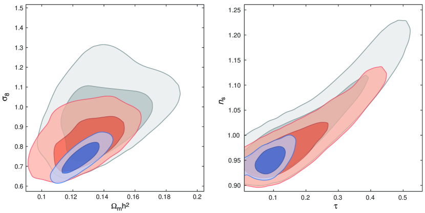
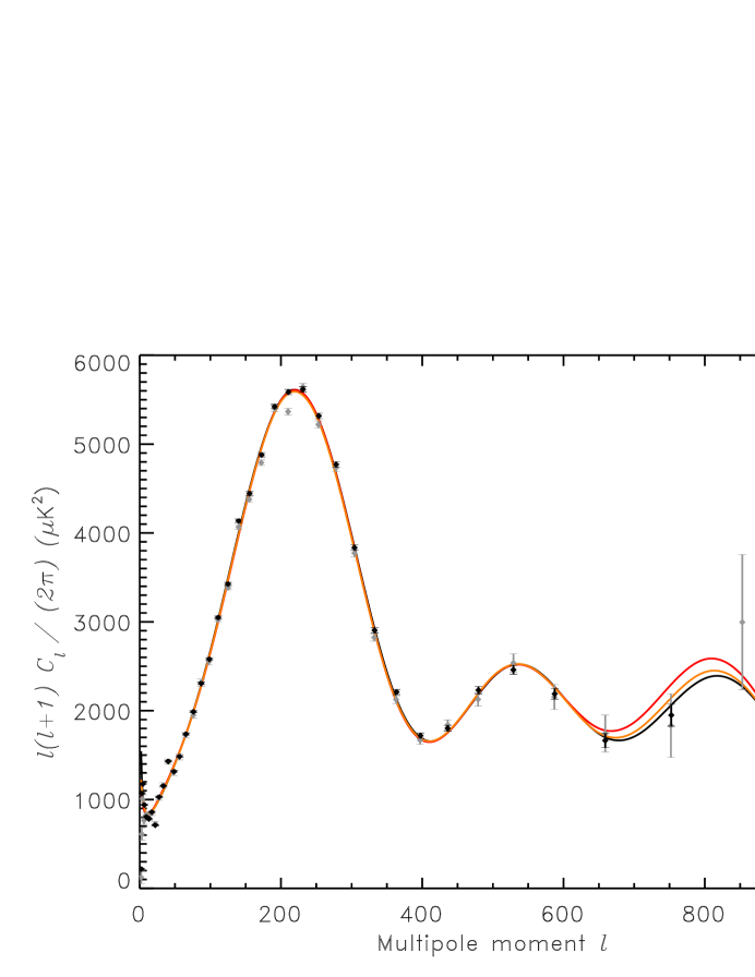
The CDM model is still an excellent fit to the WMAP data. With longer integration times and smaller pixels, the errors in the high temperature multipoles have shrunk by more than a factor of three. As the data have improved, the likelihood function remains peaked around the maximum likelihood peak of the first year WMAP value. With longer integration, the most discrepant high points from the year-one data are now much closer to the best fit model (see Figure 2). For the first year WMAP TT and TE data (Spergel et al., 2003), the reduced was 1.09 for 893 degrees of freedom (D.O.F.) for the TT data and was 1.066 for the combined TT and TE data (893+449=1342 D.O.F.). For the three year data, which has much smaller errors for , the reduced for 982 D.O.F. (- 7 parameters) is now 1.068 for the TT data and 1.041 for the combined TT and TE data ( 1410 D.O.F., including TE ), where the TE data contribution is evaluated from .
For the T, Q, and U maps using the pixel based likelihood we obtain a reduced for 1838 pixels (corresponding to for and for ). The combined reduced for 3162 degrees of freedom for the combined fit to the and power spectrum at high and the and maps at low .
While many of the maximum likelihood parameter values (Table 2, columns 3 and 7 and Figure 1) have not changed significantly, there has been a noticeable reduction in the marginalized value for the optical depth, , and a shift in the best fit value of . (Each shift is slightly larger than ). The addition of the EE data now eliminates a large region of parameter space with large and that was consistent with the first year data. With only the first year data set, the likelihood surface was very flat. It covered a ridge in over a region that extended from to nearly . If the optical depth of the universe were as large as (a value consistent with the first year data), then the measured EE signal would have been 10 times larger than the value reported in Page et al. (2006). On the other hand, an optical depth of would produce one quarter of the detected EE signal. As discussed in Page et al. (2006), the reionization signal is now based primarily on the EE signal rather than the TE signal. See figure 26 in Page et al. (2006) for the likelihood plot for : note that the form of this likelihood function is relatively insensitive to the cosmological model (over the range considered in this paper).
There has also been a significant reduction in the uncertainties in the matter density, . With the first year of WMAP data, the third peak was poorly constrained (see the light gray data points in Figure 2). With three years of integration, the WMAP data better constrain the height of the third peak: WMAP is now cosmic variance limited up to and the signal-to-noise ratio exceeds unity up to . The new best fit WMAP-only model is close to the WMAP (first year)+CBI+ACBAR model in the third peak region. As a result, the preferred value of now shifts closer to the “WMAPext” value reported in Spergel et al. (2003). Figure 1 shows the likelihood surfaces for the first year WMAP data, the first year WMAPext data and the three year WMAP data. The accurately determined peak position constrains (Page et al., 2003a), fixes the cosmological age, and determines the direction of the degeneracy surface. With 1 year data, the best fit value is . With three years of data, the best fit shifts to . The lower third peak implies a smaller value of and because of the peak constraint, a lower value of .
The best fit value of (marginalized over the other parameters) is now noticeably smaller for the three year data alone, than for the first-year WMAP data alone, . This lower value is due to a smaller third peak height, which leads to a lower value of , and less structure growth and a lower best fit value for . The height of the third peak was very uncertain with the first-year data alone. In Spergel et al. (2003), we used external CMB data sets to constrain the third peak and with these data, the Maximum Likelihood value was 0.84. With three years of data, the third peak is better determined and its height is close to the value estimated from the ground based data. With the EE measurements, we have eliminated most of the high region of parameter space. Since higher values of imply a higher amplitude of primordial fluctuations, the best fit value of is proportional to . For a model with all other parameters fixed, implies a 7% lower value of . As discussed in §4.1, this lower value of is more consistent with the X-ray measurements but lower than the best fit value from recent lensing surveys. Lower implies later growth of structure.
In the first year data, we assumed that the SZ contribution to the WMAP data was negligible. Appendix A discusses the change in priors and the change in the SZ treatment and their effects on parameters: marginalizing over SZ most significantly shifts and by 1% and 3% respectively. In Table 2 in the column labeled No SZ and Figure 1, we assume and use the first year likelihood code to make a consistent comparison between the first-year and three-year results. As in the first year analysis, we use a flat prior on the logarithm of the amplitude and a flat prior on and a flat prior on . The first column of Table 5 list the parameters fit to the WMAP three-year data with allowed to vary between 0 and 2. In the tables, the “mean” value is calculated according to equation (1) and the “Maximum Likelihood (ML)” value is the value at the peak of the likelihood function. In the last two columns, we provide our current best estimate of parameters including SZ marginalization and using the full likelihood code to compute the TT likelihoods. In subsequent tables and figures, we will allow the SZ contribution to vary and quote the appropriate marginalized values. Allowing for an SZ contribution lowers the best fit primordial contribution at high , thus, the best fit models with an SZ contribution have lower and values. However, in other tables, we use the faster likelihood code unless specifically noted. In all of the Tables, we quote the 68% confidence intervals on parameters and the 95% confidence limits on bounded parameters.
| Parameter | First Year | WMAPext | Three Year | Three Year | Three Year+ALL |
|---|---|---|---|---|---|
| Mean | Mean | Mean (No SZ) | Mean | Mean | |
| Parameter | First Year | WMAPext | Three Year | Three Year | Three Year + ALL |
| ML | ML | ML (No SZ) | ML | ML | |
3.2 Reionization History
Since the Kogut et al. (2003) detection of , the physics of reionization has been a subject of extensive theoretical study (Cen, 2003; Ciardi et al., 2003; Haiman & Holder, 2003; Madau et al., 2004; Oh & Haiman, 2003; Venkatesan et al., 2003; Ricotti & Ostriker, 2004; Sokasian et al., 2004; Somerville & Livio, 2003; Wyithe & Loeb, 2003; Iliev et al., 2005). Page et al. (2006) provides a detailed discussion of the new polarization data: while the best fit value for has not changed significantly, the new EE data, combined with an improved treatment of the TE data, implies smaller marginalized maximum likelihood value. The three year data favors , consistent with the predictions of a number of simulations of CDM models. For example, Ciardi et al. (2003) CDM simulations predict for parameters consistent with the WMAP primordial power spectrum. Tumlinson et al. (2004) use the nucleosynthetic data to derive and construct an initial mass function (IMF) for reionization and find . Chiu, Fan & Ostriker (2003) found that their joint analysis of the WMAP and SDSS quasar data favored a model with , and , very close to our new best fit values. Wyithe & Cen (2006) predict that if the product of star formation efficiency and escape fraction for Pop-III stars is comparable to that for Pop-II stars, with reionization histories characterized by an extended ionization plateau from They argue that this result holds regardless of the redshift where the intergalactic medium (IGM) becomes enriched with metals.
Measurements of the EE and TE power spectrum are a powerful probe of early star formation and an important complement to other astronomical measurements. Observations of galaxies (Malhotra & Rhoads, 2004), quasars (Fan et al., 2005) and gamma ray bursts (Totani et al., 2005) imply that the universe was mostly ionized by . The detection of large-scale TE and EE signal (Page et al., 2006) implies that the universe was mostly reionized at even higher redshift. CMB observations have the potential to constrain some of the details of reionization, as the shape of the CMB EE power spectrum is sensitive to reionization history (Kaplinghat et al., 2003; Hu & Holder, 2003). Here, we explore the ability of the current EE data to constrain reionization by postulating a two stage process as a toy model. During the first stage, the universe is partially reionized at redshift and complete reionization occurs at :
| (3) | |||||
We have modified CAMB to include this reionization history.
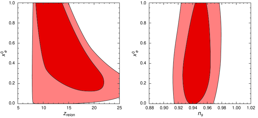
Figure 3 shows the likelihood surface for and . The plot shows that the data does not yet constrain and that the characteristic redshift of reionization is sensitive to our assumptions about reionization. If we assume that the universe is fully reionized, , then the maximum likelihood peak is . The maximum likelihood peak value of the cosmic age at the reionization epoch is
Reionization alters the TT power spectrum by suppressing fluctuations on scales smaller than the horizon size at the epoch of reionization. Without strong constraints from polarization data on , there is a strong degeneracy between spectral index and in likelihood fits (Spergel et al., 2003). The polarization measurements now strongly constrain ; however, there is still significant uncertainty in and the details of the reionization history. Fortunately, the temperature power spectrum mostly depends on the amplitude of the optical depth signal, , so that the other fit parameters (e.g., ) are insensitive to the details of the reionization history (see Figure 3). Because of this weak correlation, we will assume a simple reionization history () in all of the other analysis in this paper. Allowing for a more complex history is not likely to alter any of the conclusions of the other sections.
3.3 How Many Parameters Do We Need to Fit the WMAP Data?
| Model | |||
|---|---|---|---|
| M1 | Scale Invariant Fluctuations () | 6 | 5 |
| M2 | No Reionization () | 7.4 | 5 |
| M3 | No Dark Matter () | 248 | 6 |
| M4 | No Cosmological Constant ( | 0 | 6 |
| M5 | Power Law CDM | 0 | 6 |
| M6 | Quintessence () | 0 | 7 |
| M7 | Massive Neutrino () | -1 | 7 |
| M8 | Tensor Modes () | 0 | 7 |
| M9 | Running Spectral Index () | 7 | |
| M10 | Non-flat Universe () | 7 | |
| M11 | Running Spectral Index & Tensor Modes | 8 | |
| M12 | Sharp cutoff | 7 | |
| M13 | Binned | 20 |
In this subsection, we compare the power-law CDM to other cosmological models. We consider both simpler models with fewer parameters and models with additional physics, characterized by additional parameters. We quantify the relative goodness of fit of the models,
| (4) |
A positive value for implies the model is disfavored. A negative value means that the model is a better fit. We also characterize each model by the number of free parameters, . There are 3162 degrees of freedom in the combination of T, Q, and U maps and high TT and TE power spectra used in the fits and 1448 independent ’s, so that the effective number of data degrees of freedom is between 1448 and 3162.
Table 3 shows that the power-law CDM is a significantly better fit than the simpler models. For consistency, all of the models are computed with the likelihood code and the higher value of the point source amplitude. If we reduce the number of parameters in the model, the cosmological fits significantly worsen:
-
•
Cold dark matter serves as a significant forcing term that changes the acoustic peak structure. Alternative gravity models (e.g., MOND), and all baryons-only models, lack this forcing term so they predict a much lower third peak than is observed by WMAP and small scale CMB experiments (McGaugh, 2004; Skordis et al., 2006). Models without dark matter (even if we allow for a cosmological constant) are very poor fits to the data.
-
•
Positively curved models without a cosmological constant are consistent with the WMAP data alone: a model with the same six parameters and the prior that there is no dark energy, , fits as well as the standard model with the flat universe prior, . However, if we imposed a prior that km s-1 Mpc-1, then the WMAP data would not be consistent with . Moreover, the parameters fit to the no-cosmological-constant model, km s-1 Mpc-1 and ) are terrible fits to a host of astronomical data: large-scale structure observations, supernova data and measurements of local dynamics. As discussed in §7.3, the combination of WMAP data and other astronomical data solidifies the evidence against these models. The detected cross-correlation between CMB fluctuations and large-scale structure provides further evidence for the existence of dark energy (see §4.1.10).
-
•
The simple scale invariant () model is no longer a good fit to the WMAP data. As discussed in the previous subsection, combining the WMAP data with other astronomical data sets further strengthens the case for .
The conclusion that the WMAP data demands the existence of dark matter and dark energy is based on the assumption that the primordial power spectrum is a power-law spectrum. By adding additional features in the primordial perturbation spectrum, these alternative models may be able to better mimic the CDM model. This possibility requires further study.
The bottom half of Table 3 lists the relative improvement of the generalized models over the power-law CDM. As the Table shows, the WMAP data alone does not require the existence of tensor modes, quintessence, or modifications in neutrino properties. Adding these parameters does not improve the fit significantly. For the WMAP data, the region in likelihood space where (, , and lies within the contour. In the §7, we consider the limits on these parameters based on WMAP data and other astronomical data sets.
If we allow for a non-flat universe, then models with small negative are a better fit than the power-law CDM model. These models have a lower intervening Sachs-Wolfe (ISW) signal at low and are a better fit to the low multipoles. The best fit closed universe model has , and kmMpc-1 and is a better fit to the WMAP data alone than the flat universe model() However, as discussed in §7.3, the combination of WMAP data with either SNe data, large-scale structure data or measurements of favors models with close to 0.
In section 5, we consider several different modifications to the shape of the power spectrum. As noted in Table 3 , none of the modifications lead to significant improvements in the fit. Allowing the spectral index to vary as a function of scale improves the goodness-of-fit. The low multipoles, particularly , are lower than predicted in the CDM model. However, the relative improvement in fit is not large, , so the WMAP data alone do not require a running spectral index.
Measurement of the goodness of fit is a simple approach to test the needed number of parameters. These results should be confirmed by Bayesian model comparison techniques (Beltrán et al., 2005; Trotta, 2005; Mukherjee et al., 2006; Bridges et al., 2005). Bayesian methods, however, require an estimate of the number of data points in the fit. It is not clear whether we should use the points in the TOD, the points in the temperature maps, the points in the TT, TE, or EE power spectrum, or the numbers needed to fit the peaks and valleys in the TT data in evaluating the significance of new parameters.
4 WMAP CDM Model and Other Astronomical Data
In this paper, our approach is to show first that a wide range of astronomical data sets are consistent with the predictions of the CDM model with its parameters fitted to the WMAP data (see section §4.1). We then use the external data sets to constrain extensions of the standard model.
In our analyses, we consider several different types of data sets. We consider the SDSS LRGs, the SDSS full sample and the 2dFGRS data separately, this allows a check of systematic effects. We divide the small scale CMB data sets into low frequency experiments (CBI, VSA) and high frequency experiments (BOOMERanG, ACBAR). We divide the supernova data sets into two groups as described below. The details of the data sets are also described in §4.1.
When we consider models with more parameters, there are significant degeneracies, and external data sets are essential for parameter constraints. We use this approach in §4.2 and subsequent sections.
4.1 Predictions from the WMAP Best Fit CDM Model
The WMAP data alone is now able to accurately constrain the basic six parameters of the CDM model. In this section, we focus on this model and begin by using only the WMAP data to fix the cosmological parameters. We then use the Markov chains (and linear theory) to predict the amplitude of fluctuations in the local universe and compare to other astronomical observations. These comparisons test the basic physical assumptions of the CDM model.
4.1.1 Age of the Universe and
The CMB data do not directly measure ; however, by measuring through the height of the peaks and the conformal distance to the surface of last scatter through the peak positions (Page et al., 2003b), the CMB data produces a determination of if we assume the simple flat CDM model. Within the context of the basic model of adiabatic fluctuations, the CMB data provides a relatively robust determination of the age of the universe as the degeneracy in other cosmological parameters is nearly orthogonal to measurements of the age (Knox et al., 2001; Hu et al., 2001).
The WMAP CDM best fit value for the age: , agrees with estimates of ages based on globular clusters (Chaboyer & Krauss, 2002) and white dwarfs (Hansen et al., 2004; Richer et al., 2004). Figure 4 compares the predicted evolution of to the HST key project value (Freedman et al., 2001) and to values from analysis of differential ages as a function of redshift (Jimenez et al., 2003; Simon et al., 2005).
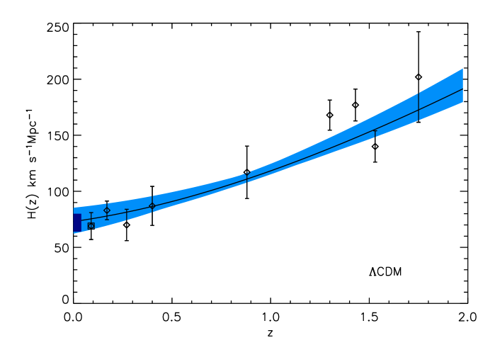
The WMAP best fit value, km/s/Mpc, is also consistent with HST measurements (Freedman et al., 2001), km/s/Mpc, where the error includes random and systematic uncertainties and the estimate is based on several different methods (Type Ia supernovae, Type II supernovae, surface brightness fluctuations and fundamental plane). It also agrees with detailed studies of gravitationally lensed systems such as B1608+656 (Koopmans et al., 2003), which yields km/s/Mpc, measurements of the Hubble constant from SZ and X-ray observations of clusters (Bonamente et al., 2005) that find km/s/Mpc, and recent measurements of the Cepheid distances to nearby galaxies that host type Ia supernova (Riess et al., 2005), km/s/Mpc.
4.1.2 Big Bang Nucleosynthesis
Measurements of the light element abundances are among the most important tests of the standard big bang model. The WMAP estimate of the baryon abundance depends on our understanding of acoustic oscillations 300,000 years after the big bang. The BBN abundance predictions depend on our understanding of physics in the first minutes after the big bang.
Table 4 lists the primordial deuterium abundance, , the primordial 3He abundance, , the primordial helium abundance, , and the primordial 7Li abundance, , based on analytical fits to the predicted BBN abundances (Kneller & Steigman, 2004) and the power-law CDM 68% confidence range for the baryon/photon ratio, . The lithium abundance is often expressed as a logarithmic abundance, [Li](Li/H).
| CMB-based BBN prediction | Observed Value | |
|---|---|---|
| 1.6 - 4.0 | ||
| (syst.) | ||
| 0.232 - 0.258 | ||
| 2.2 - 2.4 |
The systematic uncertainties in the helium abundances are due to the uncertainties in nuclear parameters, particularly neutron lifetime (Steigman, 2005). Prior to the measurements of the CMB power spectrum, uncertainties in the baryon abundance were the biggest source of uncertainty in CMB predictions. Serebrov et al. (2005) argues that the currently accepted value, s, should be reduced by s, a shift of several times the reported errors in the Particle Data Book. This (controversial) shorter lifetime lowers the predicted best fit helium abundance to (Mathews et al., 2005; Steigman, 2005).
The deuterium abundance measurements provide the strongest test of the predicted baryon abundance. Kirkman et al. (2003) estimate a primordial deuterium abundance, [D]/[H], based on five QSO absorption systems. The six systems used in the Kirkman et al. (2003) analysis show a significant range in abundances: and have a scatter much larger than the quoted observational errors. Recently, Crighton et al. (2004) report a deuterium abundance of for PKS 1937-1009. Because of the large scatter, we quote the range in [D]/[H] abundances in Table 4; however, note that the mean abundance is in good agreement with the CMB prediction.
It is difficult to directly measure the primordial 3He abundance. Bania et al. (2002) quote an upper limit on the primordial 3He abundance of . This limit is compatible with the BBN predictions.
Olive & Skillman (2004) have reanalyzed the estimates of primordial helium abundance based on observations of metal-poor HII regions. They conclude that the errors in the abundance are dominated by systematic errors and argue that a number of these systematic effects have not been properly included in earlier analysis. In Table 4, we quote their estimate of the allowed range of . Olive & Skillman (2004) find a representative value of for a linear fit of [O]/[H] to the helium abundance, significantly above earlier estimates and consistent with WMAP-normalized BBN.
While the measured abundances of the other light elements appear to be consistent with BBN predictions, measurements of neutral lithium abundance in low metallicity stars imply values that are a factor of 2 below the BBN predictions: most recent measurements (Charbonnel & Primas, 2005; Boesgaard et al., 2005) find an abundance of [Li]. While Meléndez & Ramírez (2004) find a higher value, [Li], even this value is still significantly below the BB-predicted value, . These discrepancies could be due to systematics in the inferred lithium abundance (Steigman, 2005), uncertainties in the stellar temperature scale (Fields et al., 2005), destruction of lithium in an early generation of stars or the signature of new early universe physics (Coc et al., 2004; Jedamzik, 2004; Richard et al., 2005; Ellis et al., 2005; Larena et al., 2005; Jedamzik et al., 2005). The recent detection (Asplund et al., 2005) of 6Li in several low metallicity stars further constrains chemical evolution models and exacerbates the tensions between the BBN predictions and observations.
4.1.3 Small Scale CMB Measurements
With the parameters of the CDM model fixed by the measurements of the first three acoustic peaks, the basic properties of the small scale CMB fluctuations are determined by the assumption of a power law for the amplitude of potential fluctuations and by the physics of Silk damping. We test these assumptions by comparing the WMAP best fit power law CDM model to data from several recent small scale CMB experiments (BOOMERanG, MAXIMA, ACBAR, CBI, VSA). These experiments probe smaller angular scales than the WMAP experiment and are more sensitive to the details of recombination and the physics of acoustic oscillations. The good agreement seen in Figure (5) suggests that the standard cosmological model is accurately characterizing the basic physics at .
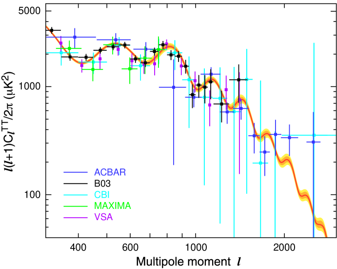
In subsequent sections, we combine WMAP with small scale experiments. We include four external CMB datasets which complement the WMAP observations at smaller scales: the Cosmic Background Imager (CBI: Mason et al. (2003); Sievers et al. (2003); Pearson et al. (2003); Readhead et al. (2004a)), the Very Small Array (VSA: Dickinson et al. (2004)), the Arcminute Cosmology Bolometer Array Receiver (ACBAR: Kuo et al. (2004)) and BOOMERanG (Ruhl et al., 2003; Montroy et al., 2005; Piacentini et al., 2005) We do not include results from a number of experiments that overlap in range coverage with WMAP as these experiments have non-trivial cross-correlations with WMAP that would have to be included in the analysis.
We do not use the small-scale polarization results for parameter determination as they do not yet noticeably improve constraints. These polarization measurements, however, already provide important tests on the basic assumptions of the model (e.g., adiabatic fluctuations and standard recombination history).
The measurements beyond the third peak improve constraints on the cosmological parameters. These observations constrict the degeneracy and provide an improved probe of a running tilt in the primordial power spectrum. In each case we only use bandpowers that do not overlap with signal-dominated WMAP observations, so that they can be treated as independent measurements.
In the subsequent sections, we perform likelihood analysis for two combinations of WMAP data with other CMB data sets: WMAP + high frequency bolometer experiments (ACBAR + BOOMERanG) and WMAP + low frequency radiometer experiments (CBI+VSA). The CBI data set is described in Readhead et al. (2004a). We use 7 band powers, with mean values of 948, 1066, 1211, 1355, 1482, 1692 and 1739, from the even binning of observations rescaled to a 32 GHz Jupiter temperature of 147.3 1.8K. The rescaling reduces the calibration uncertainty to 2.6% from 10% assumed in the first year analyses; CBI beam uncertainties scale the entire power spectrum and, thus, act like a calibration error. We use a log-normal form of the likelihood as in Pearson et al. (2003). The VSA data (Dickinson et al., 2004) uses 5 band powers with mean -values of 894, 995, 1117, 1269 and 1407, which are calibrated to the WMAP 32 GHz Jupiter temperature measurement. The calibration uncertainty is assumed to be 3% and again we use a log-normal form of the likelihood. For ACBAR (Kuo et al., 2004), we use the same band powers as in the first year analysis, with central values 842, 986, 1128, 1279, 1426, 1580, and 1716, and errors from the ACBAR web site111See http://cosmology.berkeley.edu/group/swlh/acbar/data. We assume a calibration uncertainty of 20% in , and the quoted 3% beam uncertainty in Full Width Half Maximum. We use the temperature data from the 2003 flight of BOOMERanG, based on the “NA pipeline” (Jones et al., 2005) considering the 7 datapoints and covariance matrix for bins with mean values, 924, 974, 1025, 1076, 1117, 1211 and 1370. While there is overlap between some of the small scale power spectrum measurements and WMAP measurements at , the WMAP measurements are noise-dominated so that there is little covariance between the measurements.
4.1.4 Large-Scale Structure
With the WMAP polarization measurements constraining the suppression of temperature anisotropy by reionization, we now have an accurate measure of the amplitude of fluctuations at the redshift of decoupling. If the power-law CDM model is an accurate description of the large-scale properties of the universe, then we can extrapolate forward the roughly 1000-fold growth in the amplitude of fluctuations due to gravitational clustering and compare the predicted amplitude of fluctuations to the large-scale structure observations. This is a powerful test of the theory as some alternative models fit the CMB data but predict significantly different galaxy power spectra (e.g., Blanchard et al. (2003)).
Using only the WMAP data, together with linear theory, we can predict the amplitude and shape of the matter power spectrum. The band in Figure 6 shows the 68% confidence interval for the matter power spectrum. Most of the uncertainty in the figure is due to the uncertainties in . The points in the figure show the SDSS Galaxy power spectrum (Tegmark et al., 2004b) with the amplitude of the fluctuations normalized by the galaxy lensing measurements and the 2dFGRS data (Cole et al., 2005). The figure shows that the CDM model, when normalized to observations at , accurately predicts the large-scale properties of the matter distribution in the nearby universe. It also shows that adding the large-scale structure measurements will reduce uncertainties in cosmological parameters.
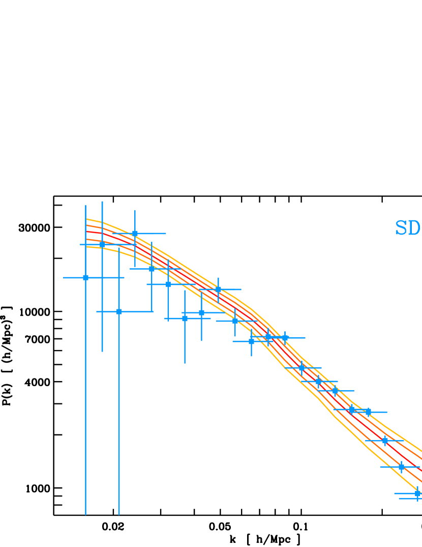
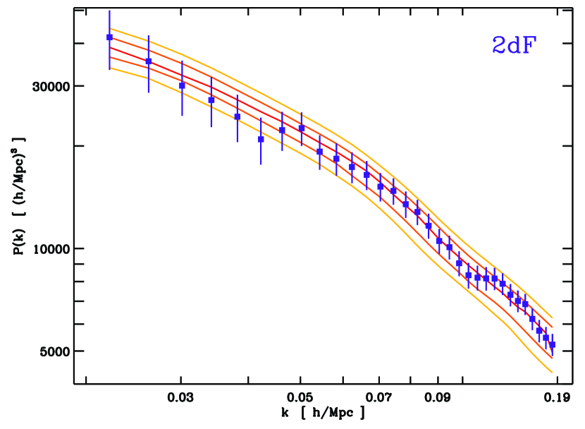
When we combine WMAP with large-scale structure observations in subsequent sections, we consider the measurements of the power spectrum from the two large-scale structure surveys. Since the galaxy power spectrum does not suffer the optical depth-driven suppression in power seen in the CMB, large scale structure data gives an independent measure of the normalization of the initial power spectrum (to within the uncertainty of the galaxy biasing and redshift space distortions) and significantly truncates the degeneracy. In addition the galaxy power spectrum shape is determined by as opposed to the dependency of the CMB. Its inclusion therefore further helps to break the or degeneracy.
The 2dFGRS survey probes the universe at redshift 0.1 (we assume for the effective redshift for the survey) and probes the power spectrum on scales MpcMpc-1. From the data and covariance described in Cole et al. (2005) we use 32 of the 36 bandpowers in the range MpcMpc-1. We correct for non-linearities and non-linear redshift space distortions using the prescription employed by the 2dF team,
| (5) |
where and are the redshift space and theoretical real space galaxy power spectra with (Mpc/h)2 and Mpc/h. We analytically marginalize over the power spectrum amplitude, effectively applying no prior on the linear bias and on linear redshift space distortions, in contrast to our first year analyses.
The SDSS main galaxy survey measures the galaxy distribution at redshift of ; however, as in the analysis of the SDSS team (Tegmark et al., 2004b) we assume , and we use 14 power spectrum bandpowers between Mpc-1. We follow the approach used in the SDSS analysis in Tegmark et al. (2004a): we use the nonlinear evolution of clustering as described in Smith et al. (2003) and include a linear bias factor, , and the linear redshift space distortion parameter, .
| (6) |
Following Lahav et al. (1991), we use where . We impose a Gaussian prior on the bias of b = 1.03 +/- 0.15, based on an estimate from weak lensing of the same SDSS galaxies used to derive the matter power spectrum. This value includes a 4% calibration uncertainty in quadrature with the reported bias error 222M. Tegmark private communication. and is a symmetrized form of the bias constraint in Table 2 of Seljak et al. (2005b). While the WMAP first year data was used in the Seljak et al. (2005b) analysis, the covariance between the data sets are small. We restrict our analysis to scales where the bias of a given galaxy population does not show significant scale dependence (Zehavi et al., 2005). Analyses that use galaxy clustering data on smaller scales require detailed modeling of non-linear dynamics and the relationship between galaxy halos and galaxy properties (see, e.g., Abazajian et al. (2005)).
The SDSS luminous red galaxy (LRG) survey uses the brightest class of galaxies in the SDSS survey (Eisenstein et al., 2005). While a much smaller galaxy sample than the main SDSS galaxy sample, it has the advantage of covering 0.72 Gpc3 between . Because of its large volume, this survey was able to detect the acoustic peak in the galaxy correlation, one of the distinctive predictions of the standard adiabatic cosmological model (Peebles & Yu, 1970; Sunyaev & Zel’dovich, 1970; Silk & Wilson, 1981; Bond & Efstathiou, 1984; Vittorio & Silk, 1984; Bond & Efstathiou, 1987). We use the SDSS acoustic peak results to constrain the balance of the matter content, using the well measured combination,
| (7) |
where is the comoving angular diameter distance and is the speed of light. We impose a Gaussian prior of based on the analysis of Eisenstein et al. (2005) .
4.1.5 Lyman Forest
Absorption features in high redshift quasars (QSO) at around the frequency of the Lyman- emission line are thought to be produced by regions of low-density gas at redshifts (Croft et al., 1998; Gnedin & Hamilton, 2002). These features allow the matter distribution to be characterized on scales of and as such extend the lever arm provided by combining large-scale structure data and CMB. These observations also probe a higher redshift range (). Thus, these observations nicely complement CMB measurements and large scale structure observations. While there has been significant progress in understanding systematics in the past few years (McDonald et al., 2005; Meiksin & White, 2004), time constraints limit our ability to consider all relevant data sets.
Recent fits to the Lyman- forest imply a higher amplitude of density fluctuations: Jena et al. (2005) find that provides a good fit to the Lyman data. Seljak et al. (2005a) combines first year WMAP data, other CMB experiments, large-scale structure and Lyman to find: and . Note that if they assume , the best fit value drops to . While these models have somewhat higher amplitudes than the new best fit WMAP values, a recent analysis by Desjacques & Nusser (2005) find that the Lyman data is consistent with between . This suggests that the Lyman data is consistent with the new WMAP best fit values; however, further analysis is needed.
4.1.6 Galaxy Motions and Properties
Observations of galaxy peculiar velocities probe the growth rate of structure and are sensitive to the matter density and the amplitude of mass fluctuations. The Feldman et al. (2003) analysis of peculiar velocities of nearby ellipticals and spirals finds and , within of the WMAP best fit value for and 1.5 higher than the WMAP value for . These estimates are based on dynamics and are not sensitive to the shape of the power spectrum. Mohayaee & Tully (2005) apply orbit retracing methods to motions in the local supercluster and obtain , consistent with the WMAP values.
Modeled galaxy properties can be compared to the clustering properties of galaxies on smaller scales. The best fit parameters for WMAP only are consistent with the recent Abazajian et al. (2005) analysis of the pre-three year release CMB data combined with the SDSS data. In their analysis, they fit a Halo Occupation Distribution model to the galaxy distribution so as to use the galaxy clustering data at smaller scales. Their best fit parameters () are consistent with the results found here. Vale & Ostriker (2005) fit the observed galaxy luminosity functions with and . Van den Bosch, Mo & Yang (2003) used the conditional luminosity function to fit the 2dFGRS luminosity function and the correlation length as a function of luminosity. Combining with the first-year WMAP data, they found and (95% CL), again in remarkable agreement with the three year WMAP best fit values.
4.1.7 Weak Lensing
Over the past few years, there has been dramatic progress in using weak lensing data as a probe of mass fluctuations in the nearby universe. Lensing surveys complement CMB measurements (Contaldi et al., 2003; Tereno et al., 2005), and their dominant systematic uncertainties differ from the large-scale structure surveys.
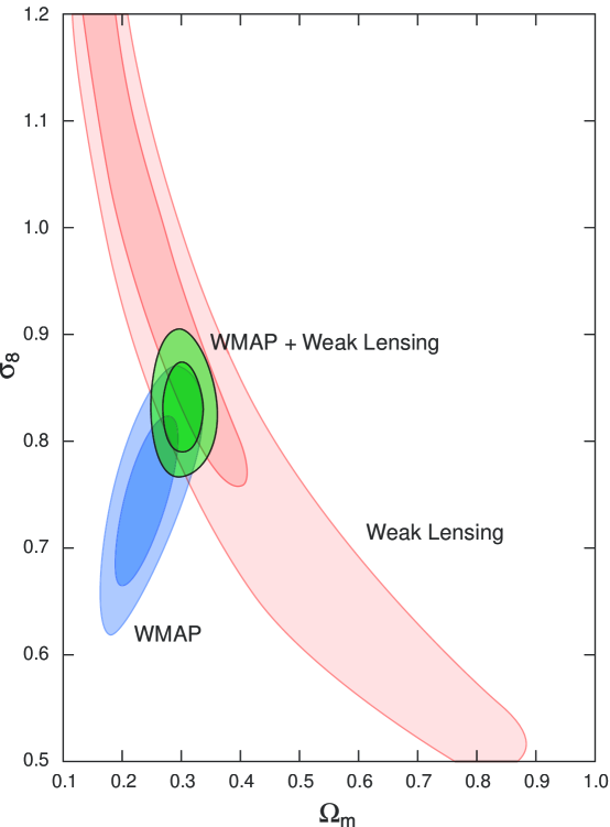
Measurements of weak gravitational lensing, the distortion of galaxy images by the distribution of mass along the line of sight, directly probe the distribution of mass fluctuations along the line of sight (see Refregier (2003) for a recent review). Figure 7 shows that the WMAP CDM model predictions for and are lower than the amplitude found in most recent lensing surveys: Hoekstra et al. (2002) calculate (95% confidence) from the RCS survey and Van Waerbeke et al. (2005) determine from the VIRMOS-DESCART survey; however, Jarvis et al. (2003) find (95% confidence level) from the 75 Degree CTIO survey.
In §4.2, we use the data set provided by the first weak gravitational lensing analysis of the Canada-France-Hawaii Telescope Legacy Survey (CFHTLS) 333http://www.cfht.hawaii.edu/Science/CFHTLS as conducted by Hoekstra et al. (2005) (Ho05) and Semboloni et al. (2005). Following Ho05, we use only the wide fields W1 and W3, hence a total area of 22 deg2 observed in the band limited to a magnitude of . We follow the same methodology as Ho05 and Tereno et al. (2005). For each given model and set of parameters, we compute the predicted shear variance at various smoothing scales, , and then evaluate its likelihood (see Ho05 equation 13).
Since the lensing data are in a noise dominated regime, we neglect the cosmological dependence of the covariance matrix. To account conservatively for a possible residual systematic contamination, we use as a monitor and add it in quadrature to the diagonal of the noise covariance matrix, as in Ho05. We furthermore marginalize over the mean source redshift, (defined in equation (16) of HoO5) assuming a uniform prior between 0.613 and 0.721. This marginalization is performed by including these extra parameters in the Monte Carlo Markov Chain. Our analysis differs however from the likelihood analysis of Ho05 in the choice of the transfer function. We use the Novosyadlyj et al. (1999)(NDL) CDM transfer function (with the assumptions of Tegmark et al. (2001)) rather than the Bardeen et al. (1986) (BBKS) CDM transfer function. The NDL transfer function includes more accurately baryon oscillations and neutrino effects. This modification alters the shape of the likelihood surface in the 2-dimensional likelihood space.
4.1.8 Strong Lensing
Strong lensing provides another potentially powerful probe of cosmology. The number of multiply-lensed arcs and quasars is very sensitive to the underlying cosmology. The cross-section for lensing depends on the number of systems with surface densities above the critical density, which in turn is sensitive to the angular diameter distance relation (Turner, 1990). The CLASS lensing survey (Chae et al., 2002) finds that the number of lenses detected in the radio survey is consistent with a flat universe with a cosmological constant and . The statistics of strong lenses in the SDSS is also consistent with the standard CDM cosmology (Oguri, 2004). The number and the properties of lensed arcs are also quite sensitive to cosmological parameters (but also to the details of the data analysis). Wambsganss et al. (2004) conclude that arc statistics are consistent with the concordance CDM model.
Soucail et al. (2004) has used multiple lenses in Abell 2218 to provide another geometrical tests of cosmological parameters. They find that and for a flat universe with dark energy. This method is another independent test of the standard cosmology.
4.1.9 Clusters and the Growth of Structure
The numbers and properties of rich clusters are another tool for testing the emerging standard model. Since clusters are rare, the number of clusters as a function of redshift is a sensitive probe of cosmological parameters. Recent analyses of both optical and X-ray cluster samples yield cosmological parameters consistent with the best fit WMAP CDM model (Borgani et al., 2001; Bahcall & Bode, 2003; Allen et al., 2003; Vikhlinin et al., 2003; Henry, 2004). The parameters are, however, sensitive to uncertainties in the conversion between observed properties and cluster mass (Pierpaoli et al., 2003; Rasia et al., 2005).
Clusters can also be used to infer cosmological parameters through measurements of the baryon/dark matter ratio as a function of redshift (Pen, 1997; Ettori et al., 2003; Allen et al., 2004). Under the assumption that the baryon/dark matter ratio is constant with redshift, the Universe is flat, and standard baryon densities, Allen et al. (2004) find and Voevodkin & Vikhlinin (2004) determine and from measurements of the baryon fraction. These parameters are consistent with the values found here and in §7.1.
4.1.10 Integrated Sachs-Wolfe (ISW) effect
The CDM model predicts a statistical correlation between CMB temperature fluctuations and the large-scale distribution of matter (Crittenden & Turok, 1996). Several groups have detected correlations between the WMAP measurements and various tracers of large-scale structure at levels consistent with the concordance CDM model (Boughn & Crittenden, 2004; Nolta et al., 2004; Afshordi et al., 2004; Scranton et al., 2003; Fosalba & Gaztañaga, 2004; Padmanabhan et al., 2005; Corasaniti et al., 2005; Boughn & Crittenden, 2005; Vielva et al., 2006). These detections provide an important independent test of the effects of dark energy on the growth of structure. However, the first year WMAP data is already signal dominated on the scales probed by the ISW effect, thus, improved large-scale structure surveys are needed to improve the statistical significance of this detection (Afshordi, 2004; Bean & Dore, 2004; Pogosian et al., 2005).
4.1.11 Supernova

With the realization that their light curve shapes could be used to make SN Ia into standard candles, supernovae have become an important cosmological probe (Phillips, 1993; Hamuy et al., 1996; Riess et al., 1996). They can be used to measure the luminosity distance as a function of redshift. The dimness of supernova provide direct evidence for the accelerating universe (Riess et al., 1998; Schmidt et al., 1998; Perlmutter et al., 1999; Tonry et al., 2003; Knop et al., 2003; Nobili et al., 2005; Clocchiatti et al., 2005; Krisciunas et al., 2005; Astier et al., 2005). Recent HST measurements (Riess et al., 2004) trace the luminosity distance/redshift relation out to higher redshift and provide additional evidence for presence of dark energy. Assuming a flat Universe, the Riess et al. (2004) analysis of the supernova data alone finds that consistent with the fits to WMAP data alone (see Table 2) and to various combinations of CMB and LSS data sets (see Tables 5 and 6). Astier et al. (2005) find that from the first year supernova legacy survey.
Within the CDM model, the supernovae data serve as a test of our cosmological model. Figure 8 shows the consistency between the supernova and CMB data. Using just the WMAP data and the CDM model, we can predict the distance/luminosity relationship and test it with the supernova data.
In §4.2 and subsequent sections, we consider two recently published high- supernovae datasets in combination with the WMAP CMB data, the first sample is 157 supernova in the “Gold Sample” as described in Riess et al. (2004) with based on a combination of ground-based data and the GOODS ACS Treasury program using the Hubble Space Telescope (HST) and the second sample is 115 supernova in the range from the Supernova Legacy Survey (SNLS) (Astier et al., 2005) .
Measurements of the apparent magnitude, , and inferred absolute magnitude, , of each SN have been used to derive the distance modulus , from which a luminosity distance is inferred, . The luminosity distance predicted from theory, , is compared to observations using a analysis summing over the SN sample.
| (8) |
where the absolute magnitude, , is a “nuisance parameter”, analytically marginalized over in the likelihood analysis (Lewis & Bridle, 2002), and contains systematic errors related to the light curve stretch factor, K-correction, extinction and the intrinsic redshift dispersion due to SNe peculiar velocities (assumed 400 and 300 km s-1 for HST/GOODS and SNLS data sets respectively).
4.2 Joint Constraints on CDM Model Parameters
| WMAP | WMAP | WMAP+ACBAR | WMAP + | |
| Only | +CBI+VSA | +BOOMERanG | 2dFGRS | |
| 100 | ||||
| WMAP+ | WMAP+ | WMAP+ | WMAP + | WMAP+ | |
| SDSS | LRG | SNLS | SN Gold | CFHTLS | |
In the previous section we showed that the power-law LCDM model fit to WMAP data only is consistent with other astronomical data. Motivated by this stringent series of cosmological tests, we combine the WMAP data with other astronomical observations to further constrain cosmological parameters.
Tables 5 and 6 show that adding external data sets has little effect on several parameters: , and . However, the various combinations do reduce the uncertainties on and the amplitude of fluctuations. The data sets used in Table 5 favor smaller values of the matter density, higher Hubble constant values, and lower values of . The data sets used in Table 6 favor higher values of , lower Hubble constants and higher values of . The lensing data is most discrepant and it most strongly pulls the combined results towards higher amplitudes and higher (see Figure 7 and 9). The overall effect of combining the data sets is shown in Figure 10.
The best fits shown in Table 6 differ by about 1 from the best fits shown in Table 5 in their predictions for the total matter density, (See Tables 5 and 6 and Figure 9). More accurate measurements of the third peak will help resolve these discrepancies.
The differences between the two sets of data may be due to statistical fluctuations. For example, the SDSS main galaxy sample power spectrum differs from the power spectrum measured from the 2dfGRS: this leads to a lower value for the Hubble constant for WMAP+SDSS data combination, , than for WMAP+2dFGRS, . Note that while the SDSS LRG data parameters values are close to those from the main SDSS catalog, they are independent determinations with mostly different systematics.
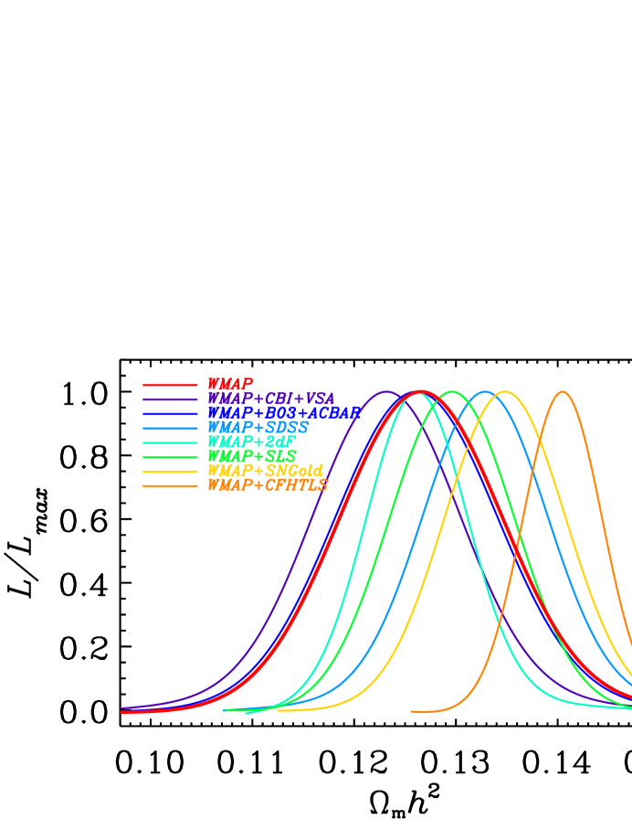
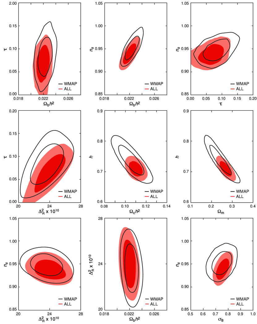
Lensing measurements are sensitive to the amplitude of the local potential fluctuations, which scale roughly as , so that lensing parameter constraints are nearly orthogonal to the CMB degeneracies (Tereno et al., 2005). The CFHTLS lensing data best fit value for is higher than the best fit three year WMAP value. As a result, the combination of CFHT and WMAP data favors a higher value of and and a lower value of than WMAP data alone. Appendix A shows that the amplitude of this discrepancy is somewhat sensitive to our choice of priors. Because of the small error bars in the CFHT data set and the relatively small overlap region in parameter space, the CFHT data set has a strong influence on cosmological parameters. Because of the small errors in the CFHT data and the relatively small overlap region in parameter space, the CFHT data has a strong influence on cosmological parameters. This effect if exacerbated when additional cosmological data sets are included in the analysis. Because of this, we do not include the lensing data in the full combined data set (WMAP…WMAP+ALL), rather we quote WMAP+CFHT results separately. The combined data sets place the strongest limits on cosmological parameters. Because they are based on the overlap between many likelihood functions, limits based on the WMAP+ALL data set should be treated with some caution. Figure 10 shows the 2-dimensional marginalized likelihood surface for both WMAP only and for the combination of WMAP+ALL.
5 Constraining the Shape of the Primordial Power Spectrum
While the simplest inflationary models predict that the spectral index varies slowly with scale, inflationary models can produce strong scale dependent fluctuations (see e.g., Kawasaki, Yamaguchi & Yokoyama (2003); Hall et al. (2004); Yamaguchi & Yokoyama (2004)). The first year WMAP observations provided some motivation for considering these models as the data, particularly when combined with the Lyman forest measurements, were better fit by models with a running spectral index (Spergel et al., 2003). Small scale CMB measurements (Readhead et al., 2004a) also favor running spectral index models over power law models.
Here, we consider whether a more general function for the primordial power spectrum could better fit the new WMAP data. We consider three forms for the power spectrum:
-
•
with a running spectral index:
-
•
allowed to freely vary in 15 bins in -space, with for . is given by linear interpolation within the bins and for .
-
•
with a sharp cut off at ,
(9)
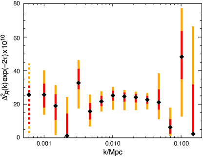
Figure 11 shows how WMAP data alone can be used to reconstruct the primordial power spectrum as a function of scale, parameterized by logarithmically spaced bins out to Mpc-1. Even allowing for these additional degrees of freedom, the data prefer a nearly featureless power-law power spectrum.
The deviation of the primordial power spectrum from a simple power law can be most simply characterized by a sharp cut-off in the primordial spectrum. Analysis of this model finds that putting in a cut off of Mpc improves the fit by , not enough to justify a radical change in the primordial spectrum.
Table 3 demonstrates that, while models with reduced large scale power provide slightly improved fits to the CMB data, the improvements do not warrant additional parameters.
5.1 External Data Sets and the Running Spectral Index
The uncertainties in the measurements of running is slightly improved by including the small scale experiments. For models with only scalar fluctuations, the marginalized value for the derivative of the spectral index is for WMAP only, for the WMAP+CBI+VSA data and for WMAP+BOOM+ACBAR. For models with tensors, for WMAP only, for WMAP+CBI+VSA, and for WMAP+BOOM+ACBAR. As Figure 12 shows, models with negative running allow large tensor amplitudes; thus, when we marginalize over with a flat prior, these models favor a more negative running.
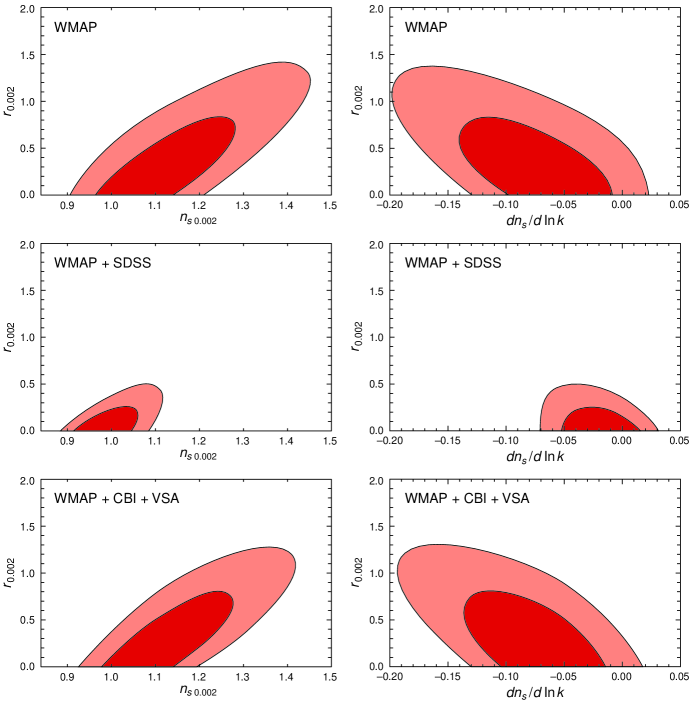
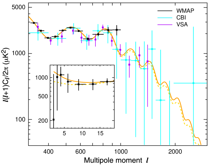
Figure 13 shows that both the power law CDM model and the running spectral index model fit the CMB data. At present, the small scale data do not yet clearly distinguish the two models.
A large absolute value of running would be problematic for most inflationary models, so further testing of this suggestive trend is important for our understanding of early universe physics. Additional WMAP data and upcoming, more sensitive small-scale CMB data will further test deviations from scale invariance. Current large scale structure data do not strengthen the case for running because these these data sets probe similar physical scales to the WMAP experiment. Figure 12 shows that current data favor a large running; however, the evidence is not yet compelling. The constraints from WMAP+lensing and WMAP+2dFGRS are similar to the WMAP+SDSS constraints shown in Figure 12.
5.2 Is the Power Spectrum Featureless?
Since inflation magnifies fluctuations that were once on sub-Planckian scales to scales of the observable horizon, trans-Planckian physics could potentially leave its imprint on the CMB sky. Over the past few years, there has been significant interest in the possibility of detecting the signature of trans-Planckian physics in the angular power spectrum. Several studies (Martin & Brandenberger, 2001; Danielsson, 2002; Easther et al., 2002; Bergström & Danielsson, 2002; Kaloper et al., 2002; Martin & Brandenberger, 2003; Martin & Ringeval, 2004; Burgess et al., 2003; Schalm, Shiu & van den Schaar, 2004) have discussed the possible form and the expected amplitude of the trans-Planckian effects which might modify the spectrum coming from slow roll inflation. The scalar power spectra resulting from power law (PL) slow roll inflation can be written in the terms of Hubble Flow parameters respectively as, (Leach & Liddle, 2003)
| (10) |
Here, and are slow roll parameters (Leach & Liddle, 2003). After the release of the first year WMAP data, Martin & Ringeval (2004) considered a primordial power spectrum of a slightly modified form to account for additional trans-Planckian (TP) features,
| (11) |
Here is determined by the Hubble parameter during inflation, , and the characteristic length scale for the trans-Planckian manifestation , and characterizes the amplitude of the trans-Planckian corrections to the fiducial spectrum. Martin & Ringeval (2004) report that the for such a model could give an improvement of 15 over the power law inflationary models for an additional 2 degrees of freedom with the first year WMAP data. With three years of data, many of the glitches and bites have disappeared, and the best fit trans-Planckian model of the form in equation (11) reduce the effective by only 4 overall and by 5 in TT relative to power law inflation, a far less significant effect.
The effect of the trans-Planckian corrections can be highly model dependent (See Easther et al. (2005a) and Easther et al. (2005b) for discussions). As an alternative, we consider forms that are more general as a way to look for oscillatory signals:
| (12) |
where or In these models, there are three new parameters: the amplitude, , the frequency, , and the phase, .
Assuming the CDM model, we fit these three parameters to the data and find reductions of 5 and 9.5 in the overall and TT . As in the Martin and Ringeval model, the improvements in the are driven by improvements in the fit around and the first peak.
6 WMAP + Inflation
The inflationary paradigm (Guth, 1981; Sato, 1981; Linde, 1982; Albrecht & Steinhardt, 1982) explains the homogeneity, isotropy and flatness of the universe by positing an early epoch of accelerated expansion. This accelerated period of expansion also generated superhorizon fluctuations (Guth & Pi, 1982; Starobinsky, 1982; Mukhanov & Chibisov, 1981; Hawking, 1982; Bardeen et al., 1983). In the simplest inflationary models, these fluctuations are Gaussian distributed in amplitude with random phase and a nearly scale invariant spectrum of fluctuations.
The detailed predictions of inflationary models depend on the properties of the inflaton potential (see Linde (2005) and Lyth & Riotto (1999) for recent reviews). Simple inflationary models predict that the slope of the primordial power spectrum, , differs from 1 and also predict the existence of a nearly scale-invariant spectrum of gravitational waves. In this section, we compare the simplest inflationary models to the WMAP three year data and to other cosmological data sets. Since we are constraining models with tensor modes, we also use the WMAP constraints on the amplitude of the B mode signal in the analysis. We characterize these models by seven basic parameters (the six basic parameters of the CDM model plus one additional parameter, , the ratio of the tensor to scalar power spectrum). Figure 14 shows the likelihood contours for the slope of the scalar fluctuations and the amplitude of the gravitational wave signal.
| Parameter | CDM + Tensor | CDM + Running +Tensors |
|---|---|---|
| set to 0 | ||
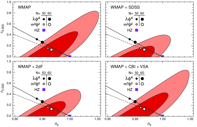
The WMAP three year data place significant constraints on inflationary models. The strength of these constraints is apparent when we consider monomial models for the inflaton potential, . These models (Lyth & Riotto, 1999) predict
| (13) |
where is the number of e-folds of inflation between the epoch when the horizon scale modes left the horizon and the end of inflation. Figure 14 compares the predictions of these monomial inflationary models to the data. For , predicts , just at the outer edge of the contour. For , predicts . However, if we allow for non-minimal gravitational couplings, then the gravity wave predictions of these models are significantly reduced (Hwang & Noh, 1998; Komatsu & Futamase, 1999) and the models are consistent with the data. Alternatively, the model is a good fit to the observations and its predicted level of gravitational waves, , is within range of upcoming experiments.
If we restrict our analysis to a specific model and value of , then the model specifies both and . In Table 8 we show the best fit parameters for the potential with . Since and are set to and for this model, there are only five free parameters ( , , , and ). The likelihood for the best fit is times higher than the best fit “Harrison Zel’dovich-Peebles” model with and . To be conservative, this comparison uses the exact (res-4) likelihood code up to and the slightly lower point source correction discussed in Appendix A. If we cut the exact likelihood off at , and use the original, higher point source value, the likelihood ratio is .
| Parameter | Mean | Best Fit |
|---|---|---|
In Peiris et al. (2003), we used the inflationary flow equations (Hoffman & Turner, 2001; Kinney, 2002) to explore the generic predictions of inflationary models. Here, we use the slow-roll approximation to explore the implications of the data for inflationary models. The results of the third year analysis are consistent with the conclusions from the first year data: while the data rule out large regions of parameter space, there are also wide range of possible inflationary models consistent with our current data. One of the most intriguing features of Figure 14 is that the data now disfavors the exact Harrison-Zel’dovich-Peebles spectrum (). For power law inflationary models, this suggests a detectable level of gravity waves. There are, however, many inflationary models that predict a much smaller gravity wave amplitude. Alternative models, such as the ekpyrotic scenario (Khoury et al., 2001, 2002) also predict an undetectable level of gravity waves.
There are several different ways of expressing the constraints that the CMB data impose on inflationary models. These parameters can be directly related to observable quantities: and . For the power law models, the WMAP bound on implies that (95% C.L.). An alternative slow roll representation (see Liddle & Lyth (1992, 1993)) uses
| (14) | |||||
| (15) |
These parameters can be related directly to observables: and . Peiris et al. (2003) discusses various classes of models in slow roll parameter space.
Models with a significant gravitational wave contributions, , make specific predictions for CMB and large-scale structure observations: (a) a modified temperature spectrum with more power at low multipoles; and (b) a lower amplitude of density fluctuations (for fixed CMB temperature fluctuations). For power law models, the strongest CMB constraints come from the shape of the temperature spectrum and the amplitude of density fluctuations. In order to fit the CMB data, models with higher values require larger values of and land a lower amplitude of scalar fluctuations, which impacts large-scale structure predictions. Thus the strongest overall constraints on the tensor mode contribution comes from the combination of CMB and large-scale structure measurements (see Table 9). These strong limits rely on our assumption of a power law spectral index. If we allow for a running index, then models with a large tensor components are consistent with the data.
| Data Set | (no running) | (with running) |
|---|---|---|
| WMAP | ||
| WMAP+BOOM+ACBAR | ||
| WMAP+CBI+VSA | ||
| WMAP+2df | ||
| WMAP+SDSS |
7 Constraining the Composition of the Universe
7.1 Dark Energy Properties
Over the past two decades, there has been growing evidence for the existence of dark energy (Peebles, 1984; Turner et al., 1984; Ostriker & Steinhardt, 1995; Dunlop et al., 1996; Krauss & Turner, 1999; Bahcall et al., 1999). By measuring both the acceleration (Riess et al., 1998; Perlmutter et al., 1999) and deceleration (Riess et al., 2004) of the universe, supernova observations provide the most direct evidence for the existence of dark energy.
The nature of this dark energy is a mystery. From a field theoretic perspective the most natural explanation for this would be the presence of a residual vacuum energy density or cosmological constant, , (Carroll et al., 1992; Peebles & Ratra, 2003). However, there are well-known fine-tuning and coincidence problems in trying to explain the 120 orders-of-magnitude discrepancy between the expected “natural” Planck-scale energy density of a cosmological constant and the observed dark energy density. These problems motivate a wide range of alternative explanations for the observations including the presence of an extra matter candidate: for example a dynamical, scalar “quintessence” field (Peebles & Ratra, 1988; Wetterich, 1988; Zlatev et al., 1999), minimally coupled (Caldwell et al., 1998; Ferreira & Joyce, 1998) or non-minimally coupled to gravity (Amendola, 1999) or other matter (Bean & Magueijo, 2001). In this latter case, the measured acceleration is due to interactions in the matter bulk. Another alternative is that modifications to gravity (e.g., Deffayet (2001); Deffayet et al. (2002)) are responsible for the observed anomalies.
The dark energy has two distinct cosmological effects: (1) through the Friedman equation, it alters the evolution of and (2) through the perturbation equations, it alters the evolution of , the growth rate of structure. The supernova data measure only the luminosity distance, which depends on , while the large scale structure data are sensitive to both and .
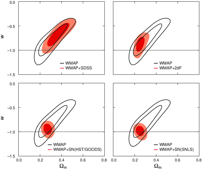
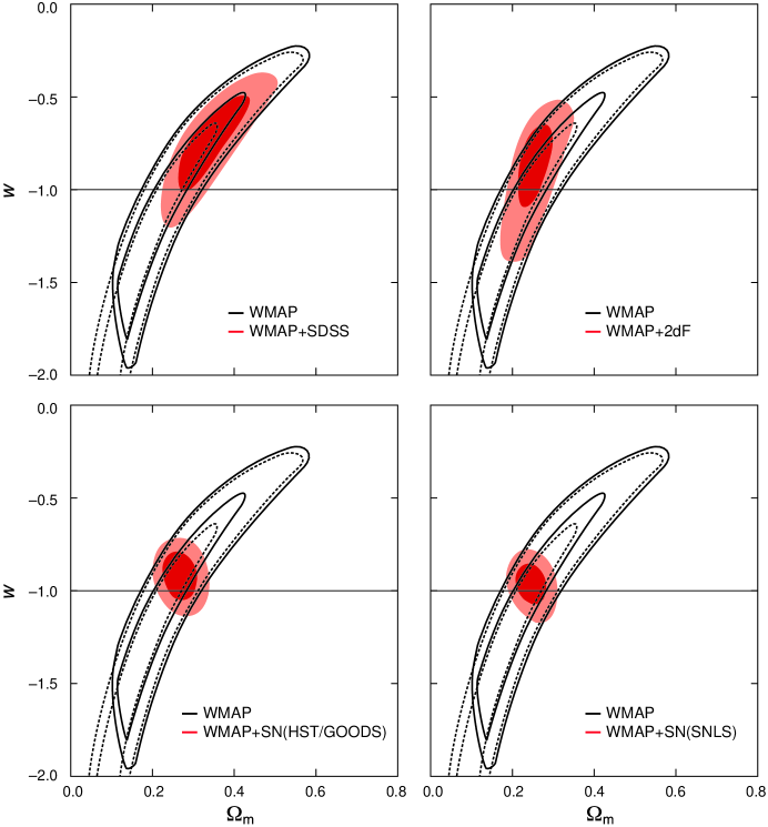
While the presence of dark energy impacts the CMB primarily through the distance to the surface of last scatter, the dark energy clustering properties also affect the CMB properties. The dark energy response to gravitational perturbations depends upon its isotropic and anisotropic sound-speeds (Hu, 1998; Bucher & Spergel, 1999). This affects the CMB fluctuations through the ISW effect. If the dark energy can cluster, then it produces a smaller ISW effect and does not enhance the power spectrum at large angular scales. These effects are most dramatic for models with , as dark energy effects in these models turn on suddenly at late times and significantly enhance the quadrupole. This can be understood in terms of the constraints imposed by the shape of the angular power spectrum: if we assume that the dark energy properties can be described by a constant value of , then fixed peak position and heights (which determine ) confine our models to a narrow valley in the likelihood surface as shown in Figure 15 and 16. The figures show that the 3 year data enable a more accurate determination of which narrows the width of the degeneracy valley. The pair of figures show that CMB data can place strong limits on models with and non-clustering dark energy. On the other hand, if the dark energy is a matter component that can cluster, even meagerly, as is the case for scalar field theories where =1, then this clustering counters the suppression of perturbation growth during the accelerative epoch and the quadrupole’s magnitude is reduced. This lessens the discriminating power of the quadrupole for measuring : while CMB data rule out the region in Figure 15, it does not constrain models in the same region in Figure 16.
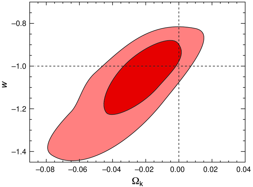
It’s interesting to note that if we relax the assumption of spatial flatness, the data still prefers models with close to (see Figure 17). In this analysis, we assume that the dark energy clusters.
| Data Set | with perturbations | no perturbations |
|---|---|---|
| WMAP + SDSS | ||
| WMAP + 2dFGRS | ||
| WMAP + SNGold | ||
| WMAP + SNLS | ||
| CMB+ LSS+ SN |
7.2 Neutrino Properties
7.2.1 Neutrino Mass
Both atmospheric neutrino and solar neutrino experiments show that neutrinos are massive and that there is significant mixing between the various neutrino interaction eigenstates (see Mohapatra et al. (2005) for a recent review). These experiments measure the difference between the square of the neutrino masses, , rather than the mass of individual neutrino mass eigenstates. Cosmological measurements nicely complement these measurements by constraining . Since light massive neutrinos do not cluster as effectively as cold dark matter, the neutrino mass has a direct impact on the amplitude and shape of the matter power spectrum (Bond et al., 1980; Bond & Szalay, 1983; Ma, 1996; Hu et al., 1998). The presence of a significant neutrino component lowers the amplitude of matter fluctuations on small scales, by roughly a factor proportional to , where is the total mass summed over neutrino species, rather than the mass of individual neutrino species. The current large-scale structure data restrict , but they are not sensitive enough to resolve the free-streaming scale of individual neutrino species (Takada et al., 2005).
Using a combination of the first year WMAP data, small-scale CMB and large-scale structure data, Spergel et al. (2003) placed an upper limit on eV. While this limit does not depend on the Lyman data, it is sensitive to galaxy bias measurements (which normalizes the large-scale structure data) and to the addition of small scale CMB data (which improves the measurement of cosmological parameters). Over the past year, several groups obtained comparable (but slightly different) limits (Hannestad, 2003; Pierpaoli, 2003; Elgarøy & Lahav, 2003). The differences are due to including (or removing) external data sets and priors or to adding additional cosmological parameters.
The limits on neutrino masses from WMAP data alone is now very close to limits based on combined CMB data sets. Ichikawa et al. (2005) used the CMB data alone to place a limit on the neutrino mass of eV. Using WMAP data alone, we now find eV.
Since the presence of massive neutrinos slows the growth of small scale structure, the combination of CMB and large-scale structure data constrain the neutrino mass. Figure 19 shows the likelihood function as a function of neutrino mass and amplitude of mass fluctuations in the local universe, . The 95% confidence limits on neutrino mass are given in Table 11. The combination of WMAP with SDSS and WMAP with 2dFGRS data constrain at roughly the same level, 20% at the 95% confidence level. This constraint yields comparable limits on the neutrino mass. While the WMAP data have improved, the error bars on have not significantly changed from the limits obtained from WMAPext + 2dFGRS, thus, the limit on neutrino mass is quite close to the first year limit. Note that in the first year analysis, we used the (Verde et al., 2002) measurement of bias for the 2dFGRS preliminary data as there had not been an equivalent analysis done for the full 2dFGRS data set. As discussed in §4.1.4, we now marginalize over the 2dFGRS bias and use the bias measurements of (Seljak et al., 2005b) for SDSS.
If the constraints on amplitude are reliable, then small scale matter power spectrum structure data can significantly improve these neutrino constraints. Goobar et al. (2006) have recently completed a CMB + Lyman study and place a limit of eV (95% C.L.). Similarly, cluster-based measurements of and lensing-based measurements of have the potential to tighten the constraint on .
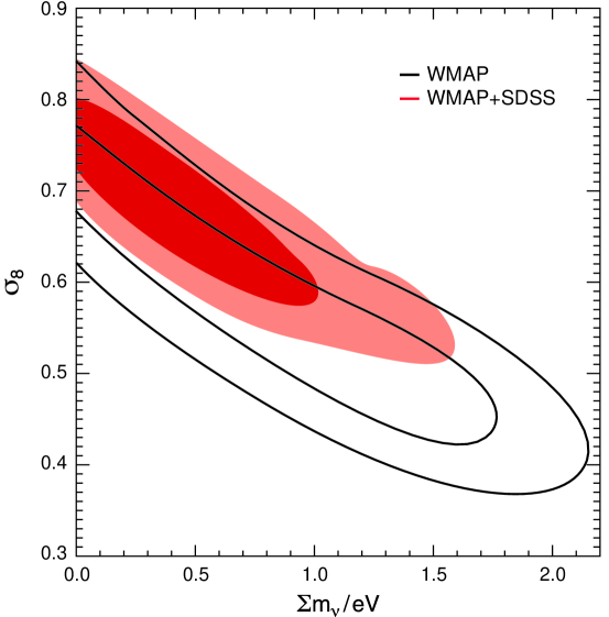
| Data Set | (95% limit for ) | |
|---|---|---|
| WMAP | ||
| WMAP + SDSS | ||
| WMAP + 2dFGRS | ||
| CMB + LSS +SN |
7.2.2 Number of Relativistic Species
If there are other light stable neutral particles (besides the three light neutrinos and the photon), then these particles will affect the CMB angular power spectrum and the evolution of large-scale structure. Because of the details of freeze-out at electron-positron annihilation (Gnedin & Gnedin, 1998; Dolgov, Hansen & Semikov, 1999), QED corrections at finite temperature (Mangano et al., 2002) and non-trivial terms in the neutrino mass matrix (Mangano et al., 2005), the effective number of neutrino species is slightly greater than 3. Any light particle that does not couple to electrons, ions and photons will act as an additional relativistic species. For neutrinos, we can compute their effects accurately as their temperature is of the CMB temperature. For other relativistic species, the limit on can be converted into a limit on their abundance by scaling by the temperature.
The shape of the CMB angular power spectrum is sensitive to the epoch of matter/radiation equality. If we increase , the effective number of neutrino species, then we will need to also increase the cold dark matter density, , and slowly change other parameters to remain consistent with the WMAP data (Bowen et al., 2002). In addition, the presence of these additional neutrino species alters the damping tail and leaves a distinctive signature on the high angular power spectrum (Bashinsky & Seljak, 2004) and on the small scale matter power spectrum.
The high matter density also alters the growth rate of structure, thus, the combination of large-scale structure and CMB data constrains the existence of any new light relativistic species. These limits constrain both the existence of new particles and the interaction properties of the neutrino (Bowen et al., 2002; Hall & Oliver, 2004). Hannestad (2001) used the pre-WMAP CMB and large-scale structure data to place an upper limit of . After the release of the first year WMAP data, several authors (Hannestad, 2003; Pierpaoli, 2003; Barger et al., 2003; Crotty et al., 2003; Elgarøy & Lahav, 2003; Barger et al., 2004; Hannestad, 2005) used the combination of WMAP, 2dFGRS and various external data to reduce this limit by a factor of 2-3. Table 11 shows the maximum likelihood estimate of the number of neutrino species for different data set combinations using the new WMAP data. The SDSS and 2dFGRS data differ in the shapes of the two measured power spectra: this difference leads to the disagreement in their best fit values for .
7.3 Non-Flat Universe
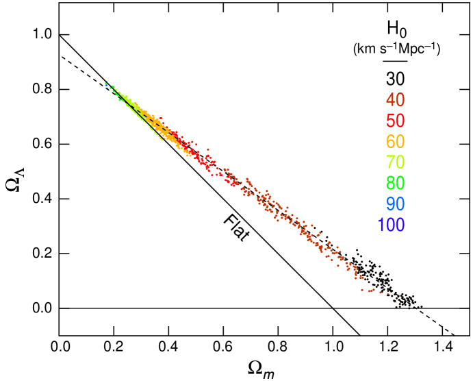
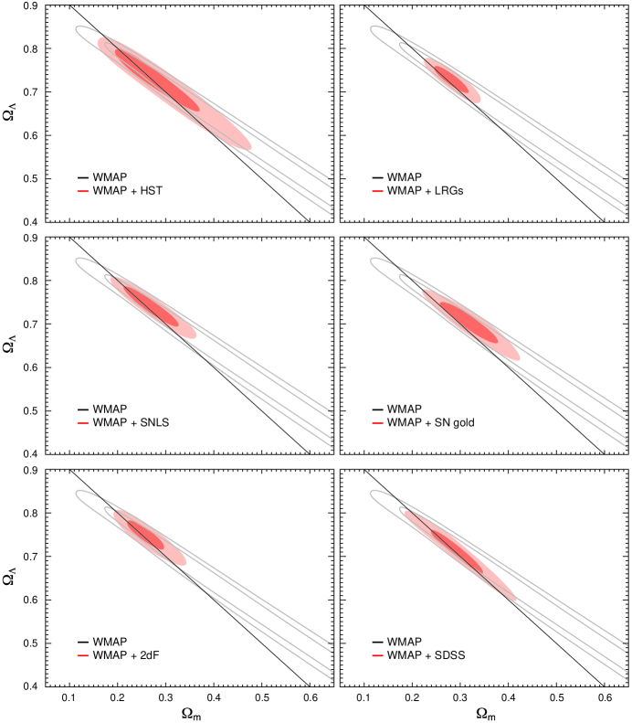
The WMAP observations place significant constraints on the geometry of the universe through the positions of the acoustic peaks. The sound horizon size, , serves as a very useful ruler for measuring the distance to the surface of last scatter. For power law open universe models, . Figure 21 shows that this constraint confines the likelihood function to a narrow degeneracy surface in . This degeneracy line is well fit by . However, the CMB data alone does not distinguish between models along the valley: it is consistent with both flat models and models with . If we allow for a large SZ signal, then the WMAP data alone favors a model with ; however, this model is not consistent with other astronomical data.
The combination of WMAP data and other astronomical data places strong constraints on the geometry of the universe (see Table 12):
-
•
The angular scale of the baryon acoustic oscillation (BAO) peak in the SDSS LRG sample (Eisenstein et al., 2005) measures the distance to . The combination of the BAO and CMB observations strongly constrain the geometry of the universe. The position of the peak in the galaxy spectrum in the SDSS and 2dFGRS surveys provide local measurements of the angular diameter distance.
-
•
Figure 20 shows that the Hubble constant varies along this line, so that the HST key project constraint on the Hubble constant leads to a strong bound on the curvature.
-
•
SNe observations measure the luminosity distance to . The combination of SNe data and CMB data also favors a nearly flat universe.
The strong limits quoted in Table 12 rely on our assumption that the dark energy has the equation of state, . In section 7.1, we discussed relaxing this assumption and assuming that is a constant. Figure 15 shows that by using the combination of CMB, large-scale structure and supernova data, we can simultaneously constrain both and . This figure confirms that our minimal model, and is consistent with the current data.
| Data Set | ||
|---|---|---|
| WMAP + | ||
| WMAP + SDSS | ||
| WMAP + 2dFGRS | ||
| WMAP + SDSS LRG | ||
| WMAP + SNLS | ||
| WMAP + SNGold |
8 Are CMB Fluctuations Gaussian?
The detection of primordial non-Gaussian fluctuations in the CMB would have a profound impact on our understanding of the physics of the early universe. While the simplest inflationary models predict only mild non-Gaussianities that should be undetectable in the WMAP data, there are a wide range of plausible mechanisms for generating significant and detectable non-Gaussian fluctuations (Bartolo et al. (2004a) for a recent review). There are a number of plausible extensions of the standard inflationary model (Lyth et al., 2003; Dvali et al., 2004; Bartolo et al., 2004b) or alternative early universe models (Arkani-Hamed et al., 2004; Alishahiha et al., 2004) that predict skewed primordial fluctuations at a level detectable by WMAP.
There are other cosmological mechanisms for generating non-Gaussianity. The smallness of the CMB quadrupole seen by both WMAP and COBE has stimulated interest in the possibility that the universe may be finite (Luminet et al., 2003; Aurich et al., 2005). If the universe were finite and had a size comparable to horizon size today, then the CMB fluctuations would be non-Gaussian (Cornish et al., 1996; Levin et al., 1997; Bond et al., 2000; Inoue et al., 2000). While analysis of the first year data did not find any evidence for a finite universe (Phillips & Kogut, 2006; Cornish et al., 2004), these searches were non-exhaustive so the data rule out most but not all small universes.
Using an analysis of Minkowski functionals, Komatsu et al. (2003) did not find evidence for statistically isotropic but non-Gaussian fluctuations in the first year sky maps . The Colley & Gott (2003) reanalysis of the maps confirmed the conclusion that there was no evidence of non-Gaussianity. Eriksen et al. (2004a) measured the Minkowski functionals and the Length of the Skeleton for the first year maps on 11 different smoothing scales. While they found no evidence for deviations from non-Gaussianity using the Minkowski area, Minkowski length and the length of the skelton, they did find a intriguingly high for the genus statistic.
For a broad class of theories, we can parameterize the effects of non-linear physics by a simple coupling term that couples a Gaussian random field, , to the Bardeen curvature potential, :
| (16) |
Simple inflationary models based on a single slowly-rolling scalar field with the canonical kinetic Lagrangian predict (Maldacena, 2003; Bartolo et al., 2004a); however, curvaton inflation (Lyth et al., 2003), ghost inflation (Arkani-Hamed et al., 2004), and Dirac-Born-Infeld (DBI) inflation models (Alishahiha et al., 2004) can generate much larger non-Gaussianity, . Using the WMAP first year data, Komatsu et al. (2003) constrained at the 95% confidence level. Several different groups (Gaztañaga & Wagg, 2003; Mukherjee & Wang, 2003; Cabella et al., 2004; Phillips & Kogut, 2006; Creminelli et al., 2005) have applied alternative techniques to measure from the maps and have similar limits on . Babich et al. (2004) note that these limits are sensitive to the physics that generated the non-Gaussianity as different mechanisms predict different forms for the bispectrum.
Since the release of the WMAP data, several groups have claimed detections of significant non-Gaussianities (Tegmark et al., 2003; Eriksen et al., 2004b; Copi et al., 2003; Vielva et al., 2004; Hansen et al., 2004; Park, 2004; Larson & Wandelt, 2004; Cruz et al., 2005). Almost all of these claims imply that the CMB fluctuations are not stationary and claim a preferred direction or orientation in the data. Hajian et al. (2005) argue that these detections are based on a posteriori selection of preferred directions and do not find evidence for preferred axes or directions. Because of the potential revolutionary significance of these detections, they must be treated with some caution. Galactic foregrounds are non-Gaussian and anisotropic, and even low level contamination in the maps can produce detectable non-Gaussianities (Chiang et al., 2003; Naselsky et al., 2005), but have only minimal effects on the angular power spectrum (Hinshaw et al., 2003). Similarly, point sources can be a source of non-Gaussianity at small angular scales (Eriksen et al., 2004b). Because of the WMAP scan pattern, the variance in the noise in the maps is spatially variable. There is significant noise in several of the Difference Assemblies (DAs) (particularly W4)— which leads to anisotropies in the two-point function of the noise. Finally, most of the claimed detections of significant non-Gaussianities are based on a posteriori statistics. Many of the claimed detections of non-Gaussianity can be tested with the three year WMAP data (available at lambda.gsfc.nasa.gov). Future tests should use the simulated noise maps, Monte Carlo simulations and the difference maps (year 1 year 2, year 2 year 3, etc.) to confirm that the tests are not sensitive to noise statistics and the multi-frequency data to confirm that any claimed non-Gaussianity has a thermal spectrum. Claims of non-Gaussianity incorporating data close to the galactic plane (within the Kp2 cut) should be treated with caution, as the foreground corrections near the plane are large and uncertain.
The following subsections describe a number of statistical tests designed to search for non-Gaussianities in the microwave sky. All of these analyses use three year maps cleaned with the KKaHaDust templates (Hinshaw et al., 2006). We refer to these maps as the “template-cleaned maps”. In the first subsection, we show that the probability distribution function of the cleaned CMB maps is consistent with Gaussianity. In the second subsection, we show that the Minkowski functionals are consistent with expectations for Gaussian fluctuations. Next, we compute the bispectrum of the cleaned maps. The final subsection describes measurements of the four point function.
8.1 One Point Distribution Function
One of the simplest tests of non-Gaussianity is a measurement of the one point probability function. However, because the detector noise in the map is inhomogeneous (higher in the ecliptic plane and lower near the poles), this test is non-trivial. We account for the spatial variations in noise by computing a variance-normalized temperature for each pixel in a given map:
| (17) |
where is the measured temperature signal, the detector noise depends on the number of observations of a given pixel, . Here, we apply the analysis to template-cleaned maps outside the Kp2 skycut. For this analysis, we compute , the noise per observation, from the year 1 year 2 difference maps and fit , the CMB signal, to the sum of the year one and year two maps. With , the computed value is within 0.5% of the value of estimated from the time series (Jarosik et al., 2006). As we lower the resolution, the value of slowly increases with increasing pixel size. For W4, the channel with the large noise, this change is most dramatic; the value of at resolution is 6% higher than the value computed for .
Figures 22 and 23 shows the one-point distribution function of the cleaned sky maps as a function of resolution. Most of the distributions appear to be rather well fit by a Gaussian. This result is consistent with that from the area of hot and cold spots (one of the Minkowski functionals), which measures the cumulative one point probability function. However, with , there is a slight excess at negative in the first panel of Figure 23. This is due to the cold spot near and discussed by (Vielva et al., 2004) in the context of the first year data. Cruz et al. (2006) argue that there is a 1.85% probability of seeing the level of skewness and kurtosis associated with this cold spot. While this probability would increase if they allowed for variable smoothing scales, the results are intriguing and merit further investigation.
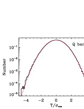

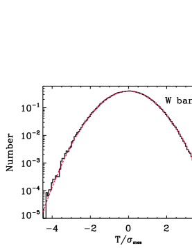
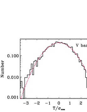
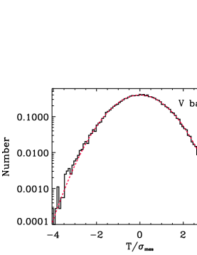
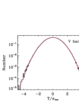
8.2 Size and Shape of Hot and Cold Spots
Minkowski functionals (Minkowski, 1903; Gott et al., 1990; Mecke, Buchert & Wagner, 1994; Schmalzing & Buchert, 1997; Schmalzing & Gorski, 1998; Winitzki & Kosowsky, 1998) measure the contour length, area, and number of hot and cold spots. Following the approach used in the first year analysis, we compute the Minkowski functionals as a function of temperature threshold, , where is the standard deviation of the map. For a two dimensional map, we measure three Minkowski functionals, the genus, , of the maps, the contour length, and the area within the contours, .
We compare the measured values of the Minkowski functionals to their expected amplitude for a Gaussian sky. We simulate a series of maps based on the best fit parameters for CDM and the WMAP noise patterns. For the analysis, we use the template-cleaned V+W maps outside the Kp0 sky mask region. Following the approach used in Komatsu et al. (2003), we compute the Minkowski functionals at 15 thresholds from to and compare each functional to the simulations using a goodness of fit statistic,
| (18) |
where is the Minkowski functional computed from the WMAP data, is the Minkowski functional computed from the simulated data, and is the bin-to-bin covariance from the simulations. Figure 24 shows the Minkowski functionals as a function of threshold for a map with (28 ′ pixels). These pixels are small enough to resolve the acoustic spots, but not so small as to be noise dominated. The figure shows that the contour length, area, and number of spots is consistent with expectations for a Gaussian theory. Table 13 lists the probability of measuring the observed values of the Minkowski functionals as a function of pixel size. At all resolutions, the maps are consistent with Gaussian simulations.
We have also simulated non-Gaussian sky with non-Gaussian signals generated according to equation (16). By comparing these simulations to the data, we can constrain at the 68% confidence level, consistent with the bispectrum measurement (§8.3).

| Pixels | Minkowski | DOF | FWMAP | ||
|---|---|---|---|---|---|
| 128 | Genus | 20.9 | 15 | 15.4 | 0.17 |
| 128 | Contour | 19.2 | 15 | 15.1 | 0.19 |
| 128 | Spot Area | 14.0 | 15 | 15.3 | 0.54 |
| 128 | Combined | 51.6 | 45 | 47.2 | 0.31 |
| 64 | Genus | 18.3 | 15 | 14.9 | 0.24 |
| 64 | Contour | 19.3 | 15 | 14.9 | 0.19 |
| 64 | Spot Area | 8.4 | 15 | 15.5 | 0.93 |
| 64 | Combined | 50.0 | 45 | 47.2 | 0.36 |
| 32 | Genus | 17.3 | 15 | 15.4 | 0.31 |
| 32 | Contour | 27.8 | 15 | 15.8 | 0.04 |
| 32 | Spot Area | 8.5 | 15 | 15.8 | 0.89 |
| 32 | Combined | 43.8 | 45 | 49.1 | 0.61 |
| 16 | Genus | 28.2 | 15 | 15.8 | 0.05 |
| 16 | Contour | 19.0 | 15 | 15.7 | 0.29 |
| 16 | Spot Area | 14.1 | 15 | 15.6 | 0.47 |
| 16 | Combined | 84.6 | 45 | 49.4 | 0.03 |
| 8 | Genus | 10.8 | 15 | 15.5 | 0.62 |
| 8 | Contour | 24.3 | 15 | 16.0 | 0.09 |
| 8 | Spot Area | 28.8 | 15 | 15.0 | 0.05 |
| 8 | Combined | 100.5 | 45 | 49.0 | 0.03 |
8.3 Bispectrum
The bispectrum is sensitive to both primordial non-Gaussianity and various sources of secondary anisotropy (Spergel & Goldberg, 1999; Goldberg & Spergel, 1999; Komatsu & Spergel, 2001). Here, we use the WMAP 3 year data to constrain the amplitude of primordial non-Gaussianity and to detect the amplitude of the point source signal in the cleaned Q, V and W band maps.
The amplitude of the primordial non-Gaussian signal can be found by computing a cubic statistic on the map (Komatsu et al., 2005):
| (19) |
where is the fraction of the sky used in the analysis, is a Weiner filtered map of the primordial fluctuations and is optimized to detect the form of the non-linearities. The amplitude of can be related directly to . Here, we use and as defined in Komatsu et al. (2005). While we used for the first-year analysis, we use for the present analysis, as noise is significantly lower with three years of data. The error on begins to increase at due to the presence of inhomogeneous noise. Note that Creminelli et al. (2005) argue that the optimal estimator for should include a term that is linear in temperature anisotropy as well as a cubic term that we already have in equation (19). They claim that their estimator could reduce the error on by about 20%. While their result is attractive, we shall not include the linear term in our analysis, as their estimator has not been tested against non-Gaussian simulations and thus it is not yet clear if it is unbiased.
Point sources are an expected cause of non-Gaussianity. Because point sources are not very correlated on the angular scales probed by WMAP, the point sources make a constant contribution to the bispectrum, . Komatsu et al. (2005) develops a cubic statistic approach for computing :
| (20) |
where , , and is a match filter optimized for point source detection:
| (21) |
where is a beam transfer function and . We weight the temperature maps by before we calculate . We use for calculating . (See § 3.2 of Komatsu et al. (2003) for details of the weighting method.) Given the uncertainties in the source cut-off and the luminosity function, the values for in Table 14 are consistent with the values of in Hinshaw et al. (2006).
Table 14 lists the measured amplitude of the non-Gaussian signals in the 3 year maps. The values are computed for template-cleaned Q, V and W band maps. With three years of data, the limits on primordial non-Gaussianity have improved from to at the 95% confidence level. The improvement in limit on is roughly consistent with the expectation that in the signal-dominated regime, (Komatsu & Spergel, 2001). The level of point source non-Gaussianity in the 3 year maps is lower than in the first year maps. This drop is due to the more sensitive 3 year masks removing additional sources.
| [] | ||
|---|---|---|
| Q | ||
| V | ||
| W | ||
| VW | ||
| QVW |
8.4 Trispectrum
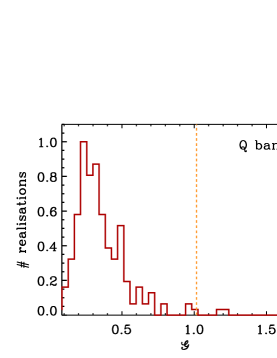
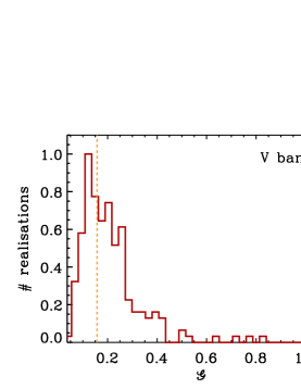
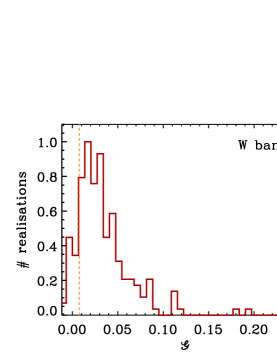
Motivated by claims that there are large scale variations in the amplitude of fluctuations, we consider a non-Gaussian model that generates a non-trivial four point function for the curvature (and temperature) fluctuations, but does not produce a three-point function. This model describes a cosmology where the value of one field modulates the amplitude of fluctuations in a second field:
| (22) |
where and are Gaussian random fields and is the Bardeen curvature potential. The presence of such a term would generate variations in the amplitude of fluctuations across the sky.
Appendix B derives an estimator for the amplitude of the non-Gaussian term, . This estimator is based on approximating the CMB fluctuations as arising from an infinitely thin surface of last scatter. We measure the amplitude of the four point function by computing
| (23) |
where is a smoothed map (e.g., an map), is an unsmoothed map, and is the expected value of for a map without any signal.
Figure 25 shows measurements of from the Q, V and W band data. The V and W band data show any evidence for a non-trivial four point function, while Q band data may show the contamination from point sources. At the S/N level of the 3 year data, there are no significant cosmological or systematic effects modulating the amplitude of the fluctuations as a function of scale.
9 Conclusions
The standard model of cosmology has survived another rigorous set of tests. The errors on the WMAP data at large are now three times smaller and there has been significant improvements in other cosmological measurements. Despite the overwhelming force of the data, the model continues to thrive. This was the basic result of (Spergel et al., 2003) and was reinforced by subsequent analyses of the first year WMAP data with the SDSS (Tegmark et al., 2004a), and analysis of first year WMAP plus the final 2dFGRS survey (Sanchez et al., 2006). After the analyses in this paper were completed, a larger SDSS LRG sample was released. An analysis of the three year WMAP data combined with the new larger sample reached the same basic conclusions as this paper: the CDM model is consistent with both CMB and large-scale structure measurements and its basic parameters are now reasonably well constrained (Tegmark et al., 2006).
The data are so constraining that there is little room for significant modifications of the basic CDM model. The combination of WMAP measurements and other astronomical measurements place significant limits on the geometry of the universe, the nature of dark energy, and even neutrino properties. While allowing for a running spectral index slightly improves the fit to the WMAP data, the improvement in the fit is not significant enough to require a new parameter.
Cosmology requires new physics beyond the standard model of particle physics: dark matter, dark energy and a mechanism to generate primordial fluctuations. The WMAP data provides insights into all three of these fundamental problems:
-
•
The clear detection of the predicted acoustic peak structure implies that the dark matter is non-baryonic.
-
•
The WMAP data are consistent with a nearly flat universe in which the dark energy has an equation of state close to that of a cosmological constant, . The combination of WMAP data with measurements of the Hubble Constant, baryon oscillations, supernova data and large-scale structure observations all reinforces the evidence for dark energy.
-
•
The simplest model for structure formation, a scale-invariant spectrum of fluctuations, is not a good fit to the WMAP data. The WMAP data requires either tensor modes or a spectral index with to fit the angular power spectrum. These observations match the basic inflationary predictions and are well fit by the predictions of the simple model.
Further WMAP observations and future analyses will test the inflationary paradigm. While we do not find convincing evidence for significant non-Gaussianities, an alternative model that better fits the low data would be an exciting development. Within the context of the inflationary models, measurements of the spectral index as a function of scale and measurements of tensor modes directly will provide a direct probe into the physics of the first moments of the big bang.
10 Acknowledgments
The WMAP mission is made possible by the support of the Office of Space Sciences at NASA Headquarters and by the hard and capable work of scores of scientists, engineers, technicians, machinists, data analysts, budget analysts, managers, administrative staff, and reviewers. We thank the referee for helpful comments, Henk Hoekstra, Yannick Mellier and Ludovic Van Waerbeke for providing the CFHTLS data and discussions of the lensing data, John Sievers for discussions of small-scale CMB experiments, Adam Riess and Kevin Kriscinius for discussion of supernova data, Daniel Eisenstein for discussion of the SDSS LRG data, Max Tegmark for discussions of SDSS P(k) data, and John Peacock for discussions about the 2dFGRS data. EK acknowledges support from an Alfred P. Sloan Research Fellowship. HVP is supported by NASA through Hubble Fellowship grant #HF-01177.01-A awarded by the Space Telescope Science Institute which is operated by the Association of Universities for Research in Astronomy, Inc., for NASA under contract NAS 5-26555. This research has made use of NASA’s Astrophysics Data System Bibliographic Services, the HEALPix software, CAMB software, and the CMBFAST software. CosmoMC (Lewis & Bridle, 2002) was used to produce Figures 1 and 26. We also used CMBWARP software (Jimenez et al., 2004) for initial investigations of the parameter space. This research was additionally supported by NASA LTSA03-000-0090, NASA ADP04-000-0093, NASA ATPNNG04GK55G, and NASA ADP05-0000-092 awards.
Appendix A SZ Marginalization, Priors, and Likelihood Approximations
In this Appendix we discuss the affect that various analysis choices have on the estimated cosmological parameters, focusing on the six parameter CDM model.
The three-year analysis now accounts for the SZ effect by marginalizing over the amplitude of the SZ contribution, parameterized by the model of Komatsu & Seljak (2002). Specifically, we evaluate their predicted spectrum using and We define the amplitude of the SZ signal (relative to this model) by and marginalize over this parameter with a flat prior, . This range is based on the assumption that the Komatsu & Seljak (2002)(KS) model estimates the true SZ signal with an uncertainty of order one. Numerical simulations (Nagai, 2005) and analytical studies (Reid & Spergel, 2006) find a tight correlation between mass and SZ signal, with uncertainties that are dominated by the cluster gas fraction. These results support the Komatsu & Seljak (2002) approach and suggest that the range of this prior is generous. Afshordi et al. (2005) analyze of the SZ signal from 116 nearby clusters in the first-year WMAP data and find that the signal from nearby clusters is 30-40% weaker than expected. Since these nearby clusters are the dominant source of fluctuations in the WMAP angular power spectrum, this implies that .
We now use the amplitude of the angular power spectrum peak, , rather than as the amplitude parameter in the Monte Carlo Markov Chains. This choice of prior leads to a slightly lower best fit amplitude.
Figure 26 shows how the SZ marginalization and the change in amplitude prior affect our estimates of cosmological parameters. Except for , the effects are all relatively small. For we estimate that roughly half of this change is due to the SZ marginalization, and half is due to the change in amplitude prior. Lewis (2006) provides a detailed study of the effects of gravitational lensing on the analysis and show that it is smaller than the SZ effect.
Since the first draft of this paper was circulated, it has been pointed out (Eriksen et al., 2006) that the pseudo--based power spectrum is biased slightly high in the range , which in turn biases the spectral index, , slightly low. As a result, we have increased the sky map resolution used in our exact TT likelihood module (to ), which allows us to use this form up to l=30. We have established that this approach agrees well with an independent exact form based on Gibbs sampling methodology (Eriksen et al., 2006).
Huffenberger et al. (2006) argue that the point source amplitude quoted in the original version of Hinshaw et al. (2006) was too high: they find , while Hinshaw et al. (2006) originally quoted . Subsequently, Hinshaw et al. (2006) have re-analyzed the source contribution and now favor an intermediate value with a more conservative error, . The original source correction also had the effect of biasing the spectral index slightly low.
Table 15 shows the sensitivity of the spectral index, , to the various treatments discussed above. The first row (Fiducial) gives the result originally quoted in this paper. The second row (No SZ Correction) gives the result if we assume . The third row (No Beam Error) shows the effect of assuming the beam window function has no error. The fourth row (Lower Point Source Amplitude) shows the change induced by changing the source amplitude (and its uncertainty) from to . The sixth row (Foreground Marginalization) shows the effect of disabling marginalization over the foreground emission template in the exact likelihood module (up to l=12). The seventh row (Res 4 Likelihood) shows the effect of using the exact likelihood module to l=30, and the last row shows our current best estimate of .
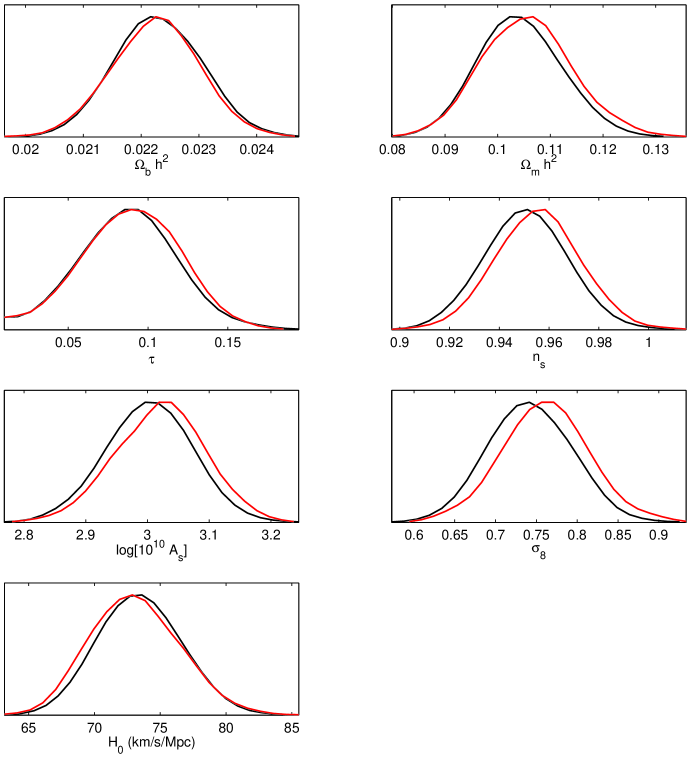
The detailed form of the likelihood function and the treatment of point sources and the SZ effect has a effect on the best fit slope. We have also used simulations where we know the input model to check the effects of including various secondary effects. Lewis (2006) provides a detailed study of the effects of gravitational lensing on the analysis and show that it is smaller than the SZ effect.
| Fiducial ( Likelihood, ) | |
|---|---|
| No SZ Correction | |
| No Beam Error | |
| Reduced Point Source Amplitude () | |
| Huffenberger et al. (2006) Point Source Amplitude () | |
| Foreground Marginalization | |
| Likelihood | |
| Likelihood + + no SZ correction | |
| Likelihood + |
Appendix B Trispectrum methodology
B.1 Predicted Trispectrum Signal
We consider here a model that generates a non-trivial trispectrum, but no bispectrum signal. We assume that the gravitational potential , is a product of two independent Gaussian fields, and :
| (B1) |
where characterizes the strength of the non-linear term.
Following Komatsu et al. (2005) approach for the bispectrum, extended recently to the trispectrum in Kogo & Komatsu (2006), the observed temperature multipoles are:
| (B2) |
where is the beam, is the noise and is the radiation transfer function:
| (B3) |
The non-linear coupling term generates a second order term:
| (B4) |
where
| (B5) |
This term does not have any effect on the bispectrum as and However, it does have a non-trivial effect on the trispectrum.
As with gravitational lensing (see Hu (2001)), the largest trispectrum term is the diagonal term, . This term would generate an excess in the of the fit of the model to the data:
| (B6) | |||||
We can then use
| (B7) |
and the equivalent relationship for to rewrite the trispectrum as
| (B8) |
where
| (B11) | |||||
While this full integral is numerically intractable, we approximate the surface of last scatter as a thin screen so that
| (B12) |
then, the trispectrum coupling term reduces to
| (B13) |
Recall that in this limit,
| (B14) |
Thus,
| (B15) |
The amplitude of is, thus, roughly the variance in the field on the scale . Note that is a positive definite quantity so that should be always positive.
B.2 Detecting the Non-Gaussian Signal
If we assume that is constant, then we can follow Hu (2001) and compute an optimal quadratic statistic. We approximate the optimal statistic as , where is a smoothed map (e.g. a res 7 map) and we use the approximation that . This has the advantage that we can easily compute it and has well-defined noise properties.
B.2.1 Practical implementations
We define for this purpose the dimensionless statistic as
where refers to various bands (Q, V, and W for yr1, yr2 and yr3) that are all distinct for a single term so that the noise bias is null for this statistic, is a particular pixel weight (we will consider it equal unity first) and is a filtered map defined as
| (B17) | |||||
| (B18) |
where ’s are the spherical harmonic coefficients of the masked sky. We use at this level the Kp12 mask to hide the brighter part of the galaxy (and potentially the brighter point sources) and ignore cut sky effects in considering those pseudo-s. But when computing the sum over pixels in , we consider only pixels outside the Kp2 area. The obvious advantage of this simple real space statistic is its ability to handle inhomogeneous noise and to localize its various contributions in real space. The second term in the definition of aims at subtracting off the Gaussian unconnected part, so that if the fields are homogeneous Gaussian fields, we obtain .
The exact nature of will depend on the source of the signal. For example, point sources do contribute to all -points functions in real or harmonic space and are as such visible in the power spectrum, bispectrum and trispectrum. The first two have been used to set limits and corrections.
Should we want to isolate the point sources contribution with the statistic, we would proceed in the following manner. The point sources power spectrum is well approximated by a constant, white noise like, power spectrum (see Komatsu et al. (2003)). Given the measured power spectrum, , the Wiener like filter to reconstruct point sources is to . Note that this filter would be optimal only if point sources were drawn from a Gaussian distribution, which is not true. We can however expect it to be close to optimal.
In order to constrain the CMB contribution to the trispectrum and constrain close to optimality, we will set and to the Wiener filter for the CMB field, and , where is the best fit model angular power spectrum and is the measured raw power spectrum including the signal and the noise and not corrected for the beam window function.
We restrict ourselves to a unit weighting which is nearly optimal in the signal dominated regime where we draw our conclusions from, i.e. at resolution lower than
B.2.2 Explicit relation to the trispectrum
References
- Abazajian et al. (2005) Abazajian, K., et al. 2005, ApJ, 625, 613
- Abroe et al. (2004) Abroe, M. E., et al. 2004, ApJ, 605, 607
- Afshordi (2004) Afshordi, N. 2004, Phys. Rev. D, 70, 083536
- Afshordi et al. (2005) Afshordi, N., Lin, Y.-T., & Sanderson, A. J. R. 2005, ApJ, 629, 1
- Afshordi et al. (2004) Afshordi, N., Loh, Y.-S., & Strauss, M. A. 2004, Phys. Rev., D69, 083524
- Albrecht & Steinhardt (1982) Albrecht, A. & Steinhardt, P. J. 1982, Phys. Rev. Lett., 48, 1220
- Alishahiha et al. (2004) Alishahiha, M., Silverstein, E., & Tong, D. 2004, Phys. Rev. D, 70, 123505
- Allen et al. (2004) Allen, S. W., Schmidt, R. W., Ebeling, H., Fabian, A. C., & van Speybroeck, L. 2004, ArXiv Astrophysics e-prints
- Allen et al. (2003) Allen, S. W., Schmidt, R. W., Fabian, A. C., & Ebeling, H. 2003, MNRAS, 342, 287
- Amendola (1999) Amendola, L. 1999, Phys. Rev. D, 60, 043501
- Arkani-Hamed et al. (2004) Arkani-Hamed, N., Creminelli, P., Mukohyama, S., & Zaldarriaga, M. 2004, Journal of Cosmology and Astro-Particle Physics, 4, 1
- Asplund et al. (2005) Asplund, M., Nissen, P. E., Lambert, D. L., Primas, F., & Smith, V. V. 2005, in IAU Symposium, ed. V. Hill, P. François, & F. Primas, 53–58
- Astier et al. (2005) Astier, P., et al. 2005, ArXiv Astrophysics e-prints
- Aurich et al. (2005) Aurich, R., Lustig, S., Steiner, F., & Then, H. 2005, Physical Review Letters, 94, 021301
- Babich et al. (2004) Babich, D., Creminelli, P., & Zaldarriaga, M. 2004, Journal of Cosmology and Astro-Particle Physics, 8, 9
- Bahcall & Bode (2003) Bahcall, N. A. & Bode, P. 2003, ApJ, 588, L1
- Bahcall et al. (1999) Bahcall, N. A., Ostriker, J. P., Perlmutter, S., & Steinhardt, P. J. 1999, Science, 284, 1481
- Bania et al. (2002) Bania, T. M., Rood, R. T., & Balser, D. S. 2002, Nature, 415, 54
- Bardeen et al. (1986) Bardeen, J. M., Bond, J. R., Kaiser, N., & Szalay, A. S. 1986, ApJ, 304, 15
- Bardeen et al. (1983) Bardeen, J. M., Steinhardt, P. J., & Turner, M. S. 1983, Phys. Rev. D, 28, 679
- Barger et al. (2003) Barger, V., Kneller, J. P., Lee, H.-S., Marfatia, D., & Steigman, G. 2003, Phys. Lett., B566, 8
- Barger et al. (2004) Barger, V., Marfatia, D., & Tregre, A. 2004, Phys. Lett., B595, 55
- Bartolo et al. (2004a) Bartolo, N., Komatsu, E., Matarrese, S., & Riotto, A. 2004a, ArXiv Astrophysics e-prints
- Bartolo et al. (2004b) Bartolo, N., Matarrese, S., & Riotto, A. 2004b, Journal of High Energy Physics, 4, 6
- Bashinsky & Seljak (2004) Bashinsky, S. & Seljak, U. 2004, Phys. Rev. D, 69, 083002
- Bean & Dore (2004) Bean, R. & Dore, O. 2004, Phys. Rev., D69, 083503
- Bean & Magueijo (2001) Bean, R. & Magueijo, J. 2001, Phys. Lett., B517, 177
- Beltrán et al. (2005) Beltrán, M., García-Bellido, J., Lesgourgues, J., Liddle, A. R., & Slosar, A. 2005, Phys. Rev. D, 71, 063532
- Bennett et al. (2003) Bennett, C. L., et al. 2003, ApJS, 148, 1
- Bergström & Danielsson (2002) Bergström, L. & Danielsson, U. H. 2002, Journal of High Energy Physics, 12, 38
- Blanchard et al. (2003) Blanchard, A., Douspis, M., Rowan-Robinson, M., & Sarkar, S. 2003, Astron. Astrophys., 412, 35
- Boesgaard et al. (2005) Boesgaard, A. M., Stephens, A., & Deliyannis, C. P. 2005, ApJ, 633, 398
- Bonamente et al. (2005) Bonamente, M., Joy, M., La Roque, S. Carlstrom, J., Reese, E., Dawson, K., ApJ, in press, astro-ph/0512349.
- Bond & Efstathiou (1984) Bond, J. R. & Efstathiou, G. 1984, ApJ, 285, L45
- Bond & Efstathiou (1987) Bond, J. R. & Efstathiou, G. 1987, MNRAS, 226, 655
- Bond et al. (1980) Bond, J. R., Efstathiou, G., & Silk, J. 1980, Physical Review Letters, 45, 1980
- Bond et al. (2000) Bond, J. R., Pogosyan, D., & Souradeep, T. 2000, Phys. Rev. D, 62, 043005
- Bond & Szalay (1983) Bond, J. R. & Szalay, A. S. 1983, ApJ, 274, 443
- Bond et al. (2005) Bond, J. R., et al. 2005, ApJ, 626, 12
- Borgani et al. (2001) Borgani, S., Rosati, P., Tozzi, P. Stanford, S.A., Eisenhardt, P.R., Lidman, C., Holden, B., Della Ceca, R., Norman, C. & Squires, G. 2001, ApJ, 561, 13.
- Boughn & Crittenden (2004) Boughn, S. & Crittenden, R. 2004, Nature, 427, 45
- Boughn & Crittenden (2005) Boughn, S. P. & Crittenden, R. G. 2005, MNRAS, 360, 1013
- Bowen et al. (2002) Bowen, R., Hansen, S. H., Melchiorri, A., Silk, J., & Trotta, R. 2002, MNRAS, 334, 760
- Bridges et al. (2005) Bridges, M., Lasenby, A. N., & Hobson, M. P. 2005, ArXiv Astrophysics e-prints
- Bucher & Spergel (1999) Bucher, M. & Spergel, D. 1999, Phys. Rev. D, 60, 043505
- Burgess et al. (2003) Burgess, C. P., Cline, J. M., Lemieux, F., & Holman, R. 2003, Journal of High Energy Physics, 2, 48
- Cabella et al. (2004) Cabella, P., Hansen, F., Marinucci, D., Pagano, D., & Vittorio, N. 2004, Phys. Rev. D, 69, 063007
- Caldwell et al. (1998) Caldwell, R. R., Dave, R., & Steinhardt, P. J. 1998, Phys. Rev. Lett., 80, 1582
- Carroll et al. (1992) Carroll, S. M., Press, W. H., & Turner, E. L. 1992, ARA&A, 30, 499
- Cen (2003) Cen, R. 2003, Astrophys. J., 591, L5
- Chaboyer & Krauss (2002) Chaboyer, B. & Krauss, L. M. 2002, ApJ, 567, L45
- Chae et al. (2002) Chae, K.-H., et al. 2002, Physical Review Letters, 89, 151301
- Charbonnel & Primas (2005) Charbonnel, C. & Primas, F. 2005, A&A, 442, 961
- Chiang et al. (2003) Chiang, L., Naselsky, P. D., Verkhodanov, O. V., & Way, M. J. 2003, ApJ, 590, L65
- Chiu, Fan & Ostriker (2003) Chiu, W. A., Fan, X. & Ostriker, J. P. 2003, ApJ599, 759
- Ciardi et al. (2003) Ciardi, B., Ferrara, A., & White, S. D. M. 2003, Mon. Not. Roy. Astron. Soc., 344, L7
- Clocchiatti et al. (2005) Clocchiatti, A., et al. 2005, ArXiv Astrophysics e-prints
- Coc et al. (2004) Coc, A., Vangioni-Flam, E., Descouvemont, P., Adahchour, A., & Angulo, C. 2004, ApJ, 600, 544
- Cole et al. (2005) Cole, S., et al. 2005, MNRAS, 362, 505
- Colley & Gott (2003) Colley, W. N. & Gott, J. R. 2003, MNRAS, 344, 686
- Contaldi et al. (2003) Contaldi, C. R., Hoekstra, H., & Lewis, A. 2003, Phys. Rev. Lett., 90, 221303
- Copi et al. (2003) Copi, C. J., Huterer, D., & Starkman, G. D. 2003, ArXiv Astrophysics e-prints
- Corasaniti et al. (2005) Corasaniti, P.-S., Giannantonio, T., & Melchiorri, A. 2005, Phys. Rev. D, 71, 123521
- Cornish et al. (1996) Cornish, N. J., Spergel, D. N., & Starkman, G. D. 1996, Physical Review Letters, 77, 215
- Cornish et al. (2004) Cornish, N. J., Spergel, D. N., Starkman, G. D., & Komatsu, E. 2004, Physical Review Letters, 92, 201302
- Creminelli et al. (2005) Creminelli, P., Nicolis, A., Senatore, L., Tegmark, M., & Zaldarriaga, M. 2005, ArXiv Astrophysics e-prints
- Crighton et al. (2004) Crighton, N. H. M., Webb, J. K., Ortiz-Gil, A., & Fernández-Soto, A. 2004, MNRAS, 355, 1042
- Crittenden & Turok (1996) Crittenden, R. G. & Turok, N. 1996, Physical Review Letters, 76, 575
- Croft et al. (1998) Croft, R. A. C., Weinberg, D. H., Katz, N., & Hernquist, L. 1998, ApJ, 495, 44
- Crotty et al. (2003) Crotty, P., Lesgourgues, J., & Pastor, S. 2003, Phys. Rev. D, 67, 123005
- Cruz et al. (2005) Cruz, M., Martínez-González, E., Vielva, P., & Cayón, L. 2005, MNRAS, 356, 29
- Cruz et al. (2006) Cruz, M., Cayon, L, Martinez-Gonzalez, E., Vielva, P. & Jin, J., astro-ph/0603859
- Danielsson (2002) Danielsson, U. H. 2002, Phys. Rev. D, 66, 023511
- de Oliveira-Costa et al. (2004) de Oliveira-Costa, A., Tegmark, M., Zaldarriaga, M., & Hamilton, A. 2004, Phys. Rev. D, 69, 063516
- Deffayet (2001) Deffayet, C. 2001, Phys. Lett. B 502, 199
- Deffayet et al. (2002) Deffayet, C., Dvali, G., & Gabadadze, G. 2002, Phys. Rev. D, 65, 044023
- Desjacques & Nusser (2005) Desjacques, V. & Nusser, A. 2005, MNRAS, 361, 1399
- Dickinson et al. (2004) Dickinson, C., et al. 2004, MNRAS, 353, 732
- Dolgov, Hansen & Semikov (1999) Dolgov, A. D., Hansen, S. H., & Semikoz, D. V. 1999, Nucl. Phys. B543, 269.
- Dunkley et al. (2005) Dunkley, J., Bucher, M., Ferreira, P.G., Moodley, K., & Skordis, C. 2005, MNRAS, 356, 925.
- Dunlop et al. (1996) Dunlop, J., Peacock, J., Spinrad, H., Dey, A., Jimenez, R., Stern, D., & Windhorst, R. 1996, Nature, 381, 581
- Dvali et al. (2004) Dvali, G., Gruzinov, A., & Zaldarriaga, M. 2004, Phys. Rev. D, 69, 083505
- Easther et al. (2002) Easther, R., Greene, B. R., Kinney, W. H., & Shiu, G. 2002, Phys. Rev. D, 66, 023518
- Easther et al. (2005a) Easther, R., Kinney, W. H., & Peiris, H. 2005a, Journal of Cosmology and Astro-Particle Physics, 8, 1
- Easther et al. (2005b) —. 2005b, Journal of Cosmology and Astro-Particle Physics, 5, 9
- Efstathiou (2004) Efstathiou, G. 2004, MNRAS, 348, 885
- Eisenstein et al. (2005) Eisenstein, D. J., et al. 2005, ApJ, 633, 560
- Elgarøy & Lahav (2003) Elgarøy, Ø. & Lahav, O. 2003, Journal of Cosmology and Astro-Particle Physics, 4, 4
- Ellis et al. (2005) Ellis, J., Olive, K. A., & Vangioni, E. 2005, Physics Letters B, 619, 30
- Eriksen et al. (2004b) Eriksen, H. K., Hansen, F. K., Banday, A. J., Górski, K. M., & Lilje, P. B. 2004b, ApJ, 605, 14
- Eriksen et al. (2004a) Eriksen, H. K., Banday, A. J., Górski, K. M., & Lilje, P. B. 2004a, ApJ, 612, 633
- Eriksen et al. (2004b) Eriksen, H. K., Novikov, D. I., Lilje, P. B., Banday, A. J., & Gorski, K. M 2004,ApJ, 612, 64
- Eriksen et al. (2006) Eriksen, H. K., Huey, G., Saha, R., Hansen, F.K., Dick, J., Banday, A. J., Gorski, K. M., Jain, P., Jewell, J. B., Knox, L., Larson, D. L., O’Dwyer, I. J., Souradeep, T. & Wandelt, B.D., Arxiv Astrophysics e-prints.
- Ettori et al. (2003) Ettori, S., Tozzi, P., & Rosati, P. 2003, A&A, 398, 879
- Fan et al. (2005) Fan, X., et al. 2005, ArXiv Astrophysics e-prints
- Feldman et al. (2003) Feldman, H., et al. 2003, ApJ, 596, L131
- Ferreira & Joyce (1998) Ferreira, P. G. & Joyce, M. 1998, Phys. Rev. D, 58, 023503
- Fields et al. (2005) Fields, B. D., Olive, K. A., & Vangioni-Flam, E. 2005, ApJ, 623, 1083
- Fosalba & Gaztañaga (2004) Fosalba, P. & Gaztañaga, E. 2004, MNRAS, 350, L37
- Freedman et al. (2001) Freedman, W. L., et al. 2001, ApJ, 553, 47
- Gaztañaga & Wagg (2003) Gaztañaga, E. & Wagg, J. 2003, Phys. Rev. D, 68, 021302
- Gelman & Rubin (1992) Gelman, A. & Rubin, D. 1992, Statistical Science, 7, 457
- Gnedin & Gnedin (1998) Gnedin, N. Y. & Gnedin, O. Y. 1998, ApJ, 509, 11
- Gnedin & Hamilton (2002) Gnedin, N. Y. & Hamilton, A. J. S. 2002, MNRAS, 334, 107
- Goldberg & Spergel (1999) Goldberg, D. M. & Spergel, D. N. 1999, Phys. Rev. D, 59, 103002
- Goobar et al. (2006) Goobar, A., Hannestad, S., Mortsell, E., & Tu, H. 2006, ArXiv Astrophysics e-prints
- Gordon et al. (2005) Gordon, C., Hu, W., Huterer, D., & Crawford, T. 2005, Phys. Rev. D, 72, 103002
- Gott et al. (1990) Gott, J. R. I., Park, C., Juszkiewicz, R., Bies, W. E., Bennett, D. P., Bouchet, F. R., & Stebbins, A. 1990, ApJ, 352, 1
- Grainge et al. (2003) Grainge, K., et al. 2003, MNRAS, 341, L23
- Guth (1981) Guth, A. H. 1981, Phys. Rev. D, 23, 347
- Guth & Pi (1982) Guth, A. H. & Pi, S. Y. 1982, Phys. Rev. Lett., 49, 1110
- Haiman & Holder (2003) Haiman, Z. & Holder, G. P. 2003, Astrophys. J., 595, 1
- Hajian & Souradeep (2003) Hajian, A. & Souradeep, T. 2003, Astrophys. J., 597, L5
- Hajian et al. (2005) Hajian, A., Souradeep, T., & Cornish, N. 2005, ApJ, 618, L63
- Hall & Oliver (2004) Hall, L. J. & Oliver, S. 2004, Nuclear Physics B Proceedings Supplements, 137, 269
- Hall et al. (2004) Hall, L. M. H., Moss, I. G., & Berera, A. 2004, Phys. Rev., D69, 083525
- Hamuy et al. (1996) Hamuy, M., Phillips, M. M., Suntzeff, N. B., Schommer, R. A., Maza, J., & Aviles, R. 1996, AJ, 112, 2391
- Hannestad (2001) Hannestad, S. 2001, Phys. Rev. D, 64, 083002
- Hannestad (2003) —. 2003, Journal of Cosmology and Astro-Particle Physics, 5, 4
- Hannestad (2005) —. 2005, ArXiv Astrophysics e-prints
- Hansen et al. (2004) Hansen, F. K., Cabella, P., Marinucci, D., & Vittorio, N. 2004, ApJ, 607, L67
- Hawking (1982) Hawking, S. W. 1982, Phys. Lett., B115, 295
- Henry (2004) Henry, J. P. 2004, ApJ, 609, 603
- Heymans et al. (2005) Heymans, C., et al. 2005, MNRAS, 361, 160
- Hinshaw et al. (2003) Hinshaw, G., et al. 2003, ApJS, 148, 135
- Hinshaw et al. (2006) Hinshaw, G. et al. 2006, ApJ, submitted
- Hoekstra et al. (2002) Hoekstra, H., Yee, H. K. C., & Gladders, M. D. 2002, ApJ, 577, 595
- Hoekstra et al. (2005) Hoekstra, H., et al. 2005, ArXiv Astrophysics e-prints
- Hoffman & Turner (2001) Hoffman, M. B. & Turner, M. S. 2001, Phys. Rev., D64, 023506
- Hu (1998) Hu, W. 1998, ApJ, 506, 485
- Hu (2001) Hu, W. 2001, in RESCEU: 1999: Birth and Evolution of the Universe, 131
- Hu et al. (1998) Hu, W., Eisenstein, D. J., & Tegmark, M. 1998, Phys. Rev. Lett., 80, 5255
- Hu et al. (2001) Hu, W., Fukugita, M., Zaldarriaga, M., & Tegmark, M. 2001, ApJ, 549, 669
- Hu & Holder (2003) Hu, W. & Holder, G. P. 2003, Phys. Rev., D68, 023001
- Huffenberger et al. (2004) Huffenberger, K. M., Seljak, U., & Makarov, A. 2004, Phys. Rev. D, 70, 063002
- Huffenberger et al. (2006) Huffenberger, K.M., Eriksen, H.K. & Hansen, F.K. 2006, ArXiv Astrophysics e-prints
- Hwang & Noh (1998) Hwang, J. & Noh, H. 1998, Physical Review Letters, Volume 81, Issue 24, December 14, 1998, pp.5274-5277, 81, 5274
- Ichikawa et al. (2005) Ichikawa, K., Fukugita, M., & Kawasaki, M. 2005, Phys. Rev. D, 71, 043001
- Iliev et al. (2005) Iliev, I. T., Mellema, G., Pen, U.-L., Merz, H., Shapiro, P. R., & Alvarez, M. A. 2005, ArXiv Astrophysics e-prints
- Inoue et al. (2000) Inoue, K. T., Tomita, K., & Sugiyama, N. 2000, MNRAS, 314, L21
- Jarosik et al. (2006) Jarosik, N. et al. 2006, ApJ, submitted
- Jarvis et al. (2003) Jarvis, M., Bernstein, G. M., Fischer, P., Smith, D., Jain, B., Tyson, J. A., & Wittman, D. 2003, AJ, 125, 1014
- Jedamzik (2004) Jedamzik, M. 2004, Phys. Rev. D, 70, 063524
- Jedamzik et al. (2005) Jedamzik, K., Choi, K.-Y.,Roszkowski, L., Ruiz de Austri, R. 2005, hep-ph/0512044
- Jena et al. (2005) Jena, T., et al. 2005, MNRAS, 361, 70
- Jimenez et al. (2004) Jimenez, R., Verde, L., Peiris, H., & Kosowsky, A. 2004, Phys. Rev., D70, 023005
- Jimenez et al. (2003) Jimenez, R., Verde, L., Treu, T., & Stern, D. 2003, Astrophys. J., 593, 622
- Jones et al. (2005) Jones, W. C., et al. 2005, ArXiv Astrophysics e-prints
- Kaloper et al. (2002) Kaloper, N., Kleban, M., Lawrence, A., Shenker, S., & Susskind, L. 2002, Journal of High Energy Physics, 11, 37
- Kaplinghat et al. (2003) Kaplinghat, M., Chu, M., Haiman, Z., Holder, G. P., Knox, L., & Skordis, C. 2003, ApJ, 583, 24
- Kawasaki, Yamaguchi & Yokoyama (2003) Kawasaki, M., Yamaguchi, M. & Yokoyama, J. 2003, Phys. Rev. D, 68, 023508.
- Khoury et al. (2002) Khoury, J., Ovrut, B. A., Seiberg, N., Steinhardt, P. J., & Turok, N. 2002, Phys. Rev., D65, 086007
- Khoury et al. (2001) Khoury, J., Ovrut, B. A., Steinhardt, P. J., & Turok, N. 2001, Phys. Rev., D64, 123522
- Kinney (2002) Kinney, W. H. 2002, Phys. Rev., D66, 083508
- Kirkman et al. (2003) Kirkman, D., Tytler, D., Suzuki, N., O’Meara, J. M., & Lubin, D. 2003, ApJS, 149, 1
- Kneller & Steigman (2004) Kneler, J. P. & Steigman, G. 2004, New Journal of Physics, 6, 117.
- Knop et al. (2003) Knop, R. A., et al. 2003, ApJ, 598, 102
- Knox et al. (2001) Knox, L., Christensen, N., & Skordis, C. 2001, ApJ, 563, L95
- Kogo & Komatsu (2006) Kogo, N. & Komatsu, E. 2006, ArXiv Astrophysics e-prints
- Kogut et al. (2003) Kogut, A., et al. 2003, ApJS, 148, 161
- Komatsu (2001) Komatsu, E. 2001, ArXiv Astrophysics e-prints, ph.D. thesis at Tohoku University (astro-ph/0206039)
- Komatsu & Futamase (1999) Komatsu, E. & Futamase, T. 1999, Phys. Rev., D59, 064029
- Komatsu & Kitayama (1999) Komatsu, E. & Kitayama, T. 1999, ApJ, 526, L1
- Komatsu & Seljak (2001) Komatsu, E. & Seljak, U. 2001, MNRAS, 327, 1353
- Komatsu & Seljak (2002) —. 2002, MNRAS, 336, 1256
- Komatsu & Spergel (2001) Komatsu, E. & Spergel, D. N. 2001, Phys. Rev. D, 63, 63002
- Komatsu et al. (2005) Komatsu, E., Spergel, D. N., & Wandelt, B. D. 2005, ApJ, 634, 14
- Komatsu et al. (2003) Komatsu, E., et al. 2003, ApJS, 148, 119
- Koopmans et al. (2003) Koopmans, L. V. E., Treu, T., Fassnacht, C. D., Blandford, R. D., & Surpi, G. 2003, ApJ, 599, 70
- Kosowsky et al. (2002) Kosowsky, A., Milosavljevic, M., & Jimenez, R. 2002, Phys. Rev. D, 66, 63007
- Krisciunas et al. (2005) Krisciunas, K., et al. 2005, AJ, 130, 2453
- Kuo et al. (2004) Kuo, C. L., et al. 2004, ApJ, 600, 32
- Krauss & Turner (1999) Krauss, L. M. & Turner, M. S. 1999, GReGr, 31, 1453
- Lahav et al. (1991) Lahav, O., Rees, M. J., Lilje, P. B., & Primack, J. R. 1991, MNRAS, 251, 128
- Land & Magueijo (2005a) Land, K. & Magueijo, J. 2005a, Phys. Rev. D, 72, 101302
- Land & Magueijo (2005b) —. 2005b, MNRAS, 362, L16
- Larena et al. (2005) Larena, J., Alimi, J.-M., & Serna, A. 2005, ArXiv Astrophysics e-prints
- Larson & Wandelt (2004) Larson, D.L., & Wandelt, B.D. 2004, ApJ, 613, L85.
- Leach & Liddle (2003) Leach, S. M. & Liddle, A. R. 2003, Phys. Rev. D, 68, 123508
- Leitch et al. (2005) Leitch, E. M., Kovac, J. M., Halverson, N. W., Carlstrom, J. E., Pryke, C., & Smith, M. W. E. 2005, ApJ, 624, 10
- Levin et al. (1997) Levin, J. J., Barrow, J. D., Bunn, E. F., & Silk, J. 1997, Physical Review Letters, 79, 974
- Lewis & Bridle (2002) Lewis, A. & Bridle, S. 2002, Phys. Rev. D, 66, 103511
- Lewis et al. (2000) Lewis, A., Challinor, A., & Lasenby, A. 2000, ApJ, 538, 473
- Lewis & Challinor (2006) Lewis, A. & Challinor, A. 2006, Phys.Rept. 429, 1.
- Lewis (2006) Lewis, A. 2006, astro-ph/0603753
- Liddle & Lyth (1992) Liddle, A. R. & Lyth, D. H. 1992, Phys. Lett., B291, 391
- Liddle & Lyth (1993) —. 1993, Phys. Rept., 231, 1
- Linde (2005) Linde, A. 2005, New Astronomy Review, 49, 35
- Linde (1982) Linde, A. D. 1982, Phys. Lett., B108, 389
- Luminet et al. (2003) Luminet, J., Weeks, J. R., Riazuelo, A., Lehoucq, R., & Uzan, J. 2003, Nature, 425, 593
- Lyth & Riotto (1999) Lyth, D. H. & Riotto, A. 1999, Phys. Rept., 314, 1
- Lyth et al. (2003) Lyth, D. H., Ungarelli, C., & Wands, D. 2003, Phys. Rev. D, 67, 23503
- Ma (1996) Ma, C.-P. 1996, ApJ, 471, 13
- Madau et al. (2004) Madau, P., Rees, M. J., Volonteri, M., Haardt, F., & Oh, S. P. 2004, Astrophys. J., 604, 484
- Maldacena (2003) Maldacena, J. 2003, Journal of High Energy Physics, 5, 13
- Mangano et al. (2002) Mangano, G., Miele, G., Pastor, S., & Peloso, S. 2002, Phys. Lett. B534, 8
- Mangano et al. (2005) Mangano, G., Miele, G., Pastor, S., Pinto, T¿, Pisanti, O. & Serpico, P. D. 2005, Nucl. Phys. B729, 221.
- Malhotra & Rhoads (2004) Malhotra, S. & Rhoads, J. E. 2004, ApJ, 617, L5
- Martin & Brandenberger (2003) Martin, J. & Brandenberger, R. 2003, Phys. Rev. D, 68, 063513
- Martin & Brandenberger (2001) Martin, J. & Brandenberger, R. H. 2001, Phys. Rev. D, 63, 123501
- Martin & Ringeval (2004) Martin, J. & Ringeval, C. 2004, Phys. Rev. D, 69, 083515
- Mason et al. (2003) Mason, B. S., et al. 2003, ApJ, 591, 540
- Mathews et al. (2005) Mathews, G. J., Kajino, T., & Shima, T. 2005, Phys. Rev. D, 71, 021302
- McDonald et al. (2005) McDonald, P., et al. 2005, ApJ, 635, 761
- McGaugh (2004) McGaugh, S. S. 2004, ApJ, 611, 26
- Mecke, Buchert & Wagner (1994) Mecke, K. R., Buchert, T., & Wagner, H. 1994, å, 388, 697.
- Meiksin & White (2004) Meiksin, A. & White, M. 2004, MNRAS, 350, 1107
- Meléndez & Ramírez (2004) Meléndez, J. & Ramírez, I. 2004, ApJ, 615, L33
- Minkowski (1903) Minkowski, H. 1903, Mathematische Annalen, 57, 447
- Mohapatra et al. (2005) Mohapatra, R. N., et al. 2005, hep-ph
- Mohayaee & Tully (2005) Mohayaee, R. & Tully, B. 2005, ApJ, 635, L113
- Montroy et al. (2005) Montroy, T. E., et al. 2005, ApJ
- Mukhanov & Chibisov (1981) Mukhanov, V. F. & Chibisov, G. V. 1981, JETP Letters, 33, 532
- Mukherjee et al. (2006) Mukherjee, P., Parkinson, D., & Liddle, A. R. 2006, ApJ, 638, L51
- Mukherjee & Wang (2003) Mukherjee, P. & Wang, Y. 2003, ApJ, 599, 1
- Nagai (2005) Nagai, D. 2005, ArXiv Astrophysics e-prints
- Naselsky et al. (2005) Naselsky, P. D., Chiang, L.-Y., Novikov, I. D., & Verkhodanov, O. V. 2005, International Journal of Modern Physics D, 14, 1273
- Nobili et al. (2005) Nobili, S., et al. 2005, A&A, 437, 789
- Nolta et al. (2004) Nolta, M. R., et al. 2004, Astrophys. J., 608, 10
- Novosyadlyj et al. (1999) Novosyadlyj, B., Durrer, R., & Lukash, V. N. 1999, A&A, 347, 799
- O’Dwyer et al. (2004) O’Dwyer, I. J. et al. 2004, Astrophys. J., 617, L99
- O’Dwyer et al. (2005) O’Dwyer, I. J., et al. 2005, ApJS, 158, 93
- Oguri (2004) Oguri, M. 2004, ArXiv Astrophysics e-prints
- Oh & Haiman (2003) Oh, S. P. & Haiman, Z. 2003, Mon. Not. Roy. Astron. Soc., 346, 456
- Olive & Skillman (2004) Olive, K. A. & Skillman, E. D. 2004, ApJ, 617, 29
- Ostriker & Steinhardt (1995) Ostriker, J. P. & Steinhardt, P. J. 1995, Nature, 377, 600
- Padmanabhan et al. (2005) Padmanabhan, N., Hirata, C. M., Seljak, U., Schlegel, D. J., Brinkmann, J., & Schneider, D. P. 2005, Phys. Rev. D, 72, 043525
- Page et al. (2003a) Page, L., et al. 2003a, ApJS, 148, 39
- Page et al. (2003b) —. 2003b, ApJS, 148, 233
- Page et al. (2006) Page, L. et al. 2006, ApJ, submitted
- Park (2004) Park, C. 2004, MNRAS, 349, 313
- Pearson et al. (2003) Pearson, T. J., et al. 2003, ApJ, 591, 556
- Peebles & Ratra (2003) Peebles, P. J. & Ratra, B. 2003, Reviews of Modern Physics, 75, 559
- Peebles (1984) Peebles, P. J. E. 1984, ApJ, 284, 439
- Peebles & Ratra (1988) Peebles, P. J. E. & Ratra, B. 1988, ApJ, 325, L17
- Peebles & Yu (1970) Peebles, P. J. E. & Yu, J. T. 1970, ApJ, 162, 815
- Peiris et al. (2003) Peiris, H. V., et al. 2003, ApJS, 148, 213
- Pen (1997) Pen, U. 1997, New Astronomy, 2, 309
- Perlmutter et al. (1999) Perlmutter, S., et al. 1999, ApJ, 517, 565
- Phillips (1993) Phillips, M. M. 1993, ApJ, 413, L105
- Phillips & Kogut (2006) Phillips, N. G. & Kogut, A. 2006, ApJ, 645, 820
- Piacentini et al. (2005) Piacentini, F., et al. 2005, ArXiv Astrophysics e-prints
- Pierpaoli (2003) Pierpaoli, E. 2003, Mon. Not. Roy. Astron. Soc., 342, L63
- Pierpaoli et al. (2003) Pierpaoli, E., Borgani, S., Scott, D., & White, M. 2003, MNRAS, 342, 163
- Pogosian et al. (2005) Pogosian, L., Corasaniti, P. S., Stephan-Otto, C., Crittenden, R., & Nichol, R. 2005, Phys. Rev. D, 72, 103519
- Prunet et al. (2005) Prunet, S., Uzan, J.-P., Bernardeau, F., & Brunier, T. 2005, Phys. Rev. D, 71, 083508
- Rasia et al. (2005) Rasia, E., Mazzotta, P., Borgani, S., Moscardini, L., Dolag, K., Tormen, G., Diaferio, A., & Murante, G. 2005, ApJ, 618, L1
- Readhead et al. (2004a) Readhead, A. C. S., et al. 2004a, ApJ, 609, 498
- Readhead et al. (2004b) —. 2004b, Science, 306, 836
- Refregier (2003) Refregier, A. 2003, ARA&A, 41, 645
- Refregier et al. (2000) Refregier, A., Komatsu, E., Spergel, D. N., & Pen, U. 2000, Phys. Rev. D, 61, 123001
- Reid & Spergel (2006) Reid, B. A. & Spergel, D. N. 2006, ArXiv Astrophysics e-prints
- Richard et al. (2005) Richard, O., Michaud, G., & Richer, J. 2005, ApJ, 619, 538
- Richer et al. (2004) Richer, H. B., et al. 2004, AJ, 127, 2904
- Ricotti & Ostriker (2004) Ricotti, M. & Ostriker, J. P. 2004, MNRAS, 352, 547
- Riess et al. (1996) Riess, A. G., Press, W. H., & Kirshner, R. P. 1996, ApJ, 473, 88
- Riess et al. (1998) Riess, A. G., et al. 1998, AJ, 116, 1009
- Riess et al. (2004) —. 2004, ApJ, 607, 665
- Riess et al. (2004) Riess, A. G. et al. 2004, Astrophys. J., 607, 665
- Riess et al. (2005) Riess, A. G., et al. 2005, ApJ, 627, 579
- Ruhl et al. (2003) Ruhl, J. E., et al. 2003, ApJ, 599, 786
- Sanchez et al. (2006) Sanchez, A., Ariel, G., Bauch, C.M., Percival, W.J, Peacock. J.A., Padilla, N.D., Cole, S., Frenk, C.S. & Norberg, P. 2006, MNRAS, 366, 189.
- Sato (1981) Sato, K. 1981, MNRAS, 195, 467
- Schalm, Shiu & van den Schaar (2004) Schalm, K., Shiu, G. & van den Schaar, J. P. 2004, JHEP, 0404, 076
- Schmalzing & Buchert (1997) Schmalzing, J. & Buchert, T. 1997, ApJ, 482, L1
- Schmalzing & Gorski (1998) Schmalzing, J. & Gorski, K. M. 1998, MNRAS, 297, 355
- Schmidt et al. (1998) Schmidt, B. P., et al. 1998, ApJ, 507, 46
- Scranton et al. (2003) Scranton, R. et al. 2003, ArXiv Astrophysics e-prints
- Seager, Sasselov & Scott (2000) Seager, S., Sasselov, D. D., Scott, D. 2000, ApJS, 128, 407
- Seljak et al. (2003) Seljak, U. et al. 2003
- Seljak et al. (2005a) Seljak, U., et al. 2005a, Phys. Rev. D, 71, 103515
- Seljak et al. (2005b) —. 2005b, Phys. Rev. D, 71, 043511
- Semboloni et al. (2005) Semboloni, E., et al. 2005, ArXiv Astrophysics e-prints
- Serebrov et al. (2005) Serebrov, A., et al. 2005, Physics Letters B, 605, 72
- Sievers et al. (2003) Sievers, J. L., et al. 2003, ApJ, 591, 599
- Silk & Wilson (1981) Silk, J. & Wilson, M.L. 1981, ApJ, 244, L37
- Simon et al. (2005) Simon, J., Verde, L., & Jimenez, R. 2005, Phys. Rev. D, 71, 123001
- Skordis et al. (2006) Skordis, C., Mota, D. F., Ferreira, P. G., & Bœhm, C. 2006, Physical Review Letters, 96, 011301
- Slosar et al. (2004) Slosar, A., Seljak, U., & Makarov, A. 2004, Phys. Rev., D69, 123003
- Slosar et al. (2003) Slosar, A., et al. 2003, MNRAS, 341, L29
- Smith et al. (2003) Smith, R. E., et al. 2003, MNRAS, 341, 1311
- Sokasian et al. (2004) Sokasian, A., Yoshida, N., Abel, T., Hernquist, L., & Springel, V. 2004, MNRAS, 350, 47
- Somerville & Livio (2003) Somerville, R. S. & Livio, M. 2003, Astrophys. J., 593, 611
- Soucail et al. (2004) Soucail, G., Kneib, J.-P., & Golse, G. 2004, A&A, 417, L33
- Spergel & Goldberg (1999) Spergel, D. N. & Goldberg, D. M. 1999, Phys. Rev. D, 59, 103001
- Spergel et al. (2003) Spergel, D. N., et al. 2003, ApJS, 148, 175
- Starobinsky (1982) Starobinsky, A. A. 1982, Phys. Lett., B117, 175
- Steigman (2005) Steigman, G. 2005, ArXiv Astrophysics e-prints
- Sunyaev & Zel’dovich (1970) Sunyaev, R. A. & Zel’dovich, Y. B. 1970, Ap&SS, 7, 3
- Takada et al. (2005) Takada, M., Komatsu, E., & Futamase, T. 2005, ArXiv Astrophysics e-prints
- Tegmark et al. (2003) Tegmark, M., de Oliveira-Costa, A., & Hamilton, A. J. 2003, Phys. Rev. D, 68, 123523
- Tegmark et al. (2001) Tegmark, M., Zaldarriaga, M., & Hamilton, A. J. 2001, Phys. Rev. D, 63, 043007
- Tegmark et al. (2004a) Tegmark, M., et al. 2004a, Phys. Rev. D, 69, 103501
- Tegmark et al. (2004b) —. 2004b, ApJ, 606, 702
- Tegmark et al. (2006) Tegmark, M., Eisenstein, D., Strauss, M., Weinberg, D., Blanton, M., Frieman, J., Fukugita, M., Gunn, J., Hamilton, A., Knapp, G., Nichol, R., Ostriker, J., Padmanabhan, N., Percival, W., Schlegel, D., Schneider, D., Scoccimarro, R., Seljak, U., Seo, H., Swanson, M., Szalay, A., Vogeley, M., Yoo, J., Zehavi, I., Abazajian, K., Anderson, S., Annis, J., Bahcall, N., Bassett, B., Berlind, A., Brinkmann, J., Budavari, T., Castander, F., Connolly, A., Csabai, I., Doi, M., Finkbeiner, D., Gillespie, B., Glazebrook, K., Hennessy, G., Hogg, D., Ivezic, Z., Jain, B., Johnston, D., Kent, S., Lamb, D., Lee, B., Lin, H., Loveday, J., Lupton, R., Munn, J., Pan, K., Park, C., Peoples, J., Pier, J., Pope, A., Richmond, M., Rockosi, C., Scranton, R., Sheth, R., Stebbins, A., Stoughton, C., Szapudi, I., Tucker, D., Vanden Berk, D., Yanny, B., York, D. 2006, astro-ph/0608032.
- Tereno et al. (2005) Tereno, I., Doré, O., van Waerbeke, L., & Mellier, Y. 2005, A&A, 429, 383
- Tomita (2005) Tomita, K. 2005, Phys. Rev. D, 72, 103506
- Tomita (2006) —. 2006, Phys. Rev. D, 73, 029901
- Tonry et al. (2003) Tonry, J. L., et al. 2003, ApJ, 594, 1
- Totani et al. (2005) Totani, T., Kawai, N., Kosugi, G., Aoki, K., Yamada, T., Iye, M., Ohta, K., & Hattori, T. 2005, ArXiv Astrophysics e-prints
- Trotta (2005) Trotta, R. 2005, ArXiv Astrophysics e-prints
- Tumlinson et al. (2004) Tumlinson, J., Vankatesan, A. & Shull, J. M. 2004, ApJ, 612, 602.
- Turner (1990) Turner, E. L. 1990, ApJ, 365, L43
- Turner et al. (1984) Turner, M. S., Steigman, G., & Krauss, L. M. 1984, Physical Review Letters, 52, 2090
- Vale & Ostriker (2005) Vale, A. & Ostriker, J. P. 2005, ArXiv Astrophysics e-prints
- Van den Bosch, Mo & Yang (2003) Van den Bosch,, F., Mo, H. & Yang, X. 2003, MNRAS, 345, 923
- Van Waerbeke et al. (2005) Van Waerbeke, L., Mellier, Y., & Hoekstra, H. 2005, A&A, 429, 75
- Venkatesan et al. (2003) Venkatesan, A., Tumlinson, J. & Shull, J. M. 2003, ApJ, 584, 608
- Verde et al. (2002) Verde, L., et al. 2002, MNRAS, 335, 432
- Verde et al. (2003) —. 2003, ApJS, 148, 195
- Vielva et al. (2004) Vielva, P., Martínez-González, E., Barreiro, R. B., Sanz, J. L., & Cayón, L. 2004, ApJ, 609, 22
- Vielva et al. (2006) Vielva, P., Martínez-González, E., & Tucci, M. 2006, MNRAS, 365, 891
- Vikhlinin et al. (2003) Vikhlinin, A., et al. 2003, ApJ, 590, 15
- Vittorio & Silk (1984) Vittorio, N. & Silk, J. 1984, ApJ, 285, L39
- Voevodkin & Vikhlinin (2004) Voevodkin, A. & Vikhlinin, A. 2004, ApJ, 601, 610
- Wambsganss et al. (2004) Wambsganss, J., Bode, P., & Ostriker, J. P. 2004, ApJ, 606, L93
- Wetterich (1988) Wetterich, C. 1988, Nucl. Phys., B302, 668
- Winitzki & Kosowsky (1998) Winitzki, S. & Kosowsky, A. 1998, New Astronomy, 3, 75
- Wyithe & Cen (2006) Wyithe, J. S. B. & Cen, R. 2006, ArXiv Astrophysics e-prints
- Wyithe & Loeb (2003) Wyithe, J. S. B. & Loeb, A. 2003, ApJ, 588, L69
- Yamaguchi & Yokoyama (2004) Yamaguchi, M. & Yokoyama, J. 2003, Phys. Rev. D, 70, 023513
- Zaldarriaga & Seljak (2000) Zaldarriaga, M. & Seljak, U. 2000, ApJS, 129, 431
- Zehavi et al. (2005) Zehavi, I., et al. 2005, ApJ, 630, 1
- Zlatev et al. (1999) Zlatev, I., Wang, L., & Steinhardt, P. J. 1999, Physical Review Letters, 82, 896