Reduction of Cosmological Data for the Detection of Time-varying Dark Energy Density

Abstract

We present a method for reducing cosmological data to constraints on the amplitudes of modes of the dark energy density as a function of redshift. The modes are chosen so that 1) one of them has constant density and 2) the others are non-zero only if there is time-variation in the dark energy density and 3) the amplitude errors for the time-varying modes are uncorrelated with each other. We apply our method to various combinations of three-year WMAP data (Spergel et al., 2006), baryon acoustic oscillation data (Eisenstein et al., 2005), the Riess et al. (2004) ’Gold’ supernova data set, and the Supernova Legacy Survey data set (Astier et al., 2005). We find no significant evidence for a time-varying dark energy density or for non-zero mean curvature. Although by some measure the limits on four of the time-varying mode amplitudes are quite tight, they are consistent with the expectation that the dark energy density does not vary on time scales shorter than a Hubble time. Since we do not expect detectable time variation in these modes, our results should be viewed as a systematic error test which the data have passed. We discuss a procedure to identify modes with maximal signal-to-noise ratio.

Submitted to JCAP

1 Introduction

That the cosmological expansion rate is accelerating is well-established. Two pressing questions, of deep importance for fundamental physics, are 1) Is the acceleration due to corrections to the gravitational field equations or to some unknown matter component that we call dark energy? and 2) If dark energy, is it a cosmological constant or something with a time-varying density? Here we present a method for reducing cosmological measurements of distance as a function of redshift in a manner suited to answering this second question.

Our method reduces cosmological data (anything that depends on the history of the dark energy density, $\rho_{x}(z)$) to constraints on a cosmological constant plus the amplitudes of time-varying modes of $\rho_{x}(z)$. The modes are chosen to have uncorrelated amplitude errors and to be those that are best determined by the data. The two chief desirable properties of such a reduction are:

1. The cosmological constraints can be expressed in a highly model-independent manner in terms of just a few numbers (plus associated functions of redshift).

2. Consistency with a cosmological constant is straightforward to study visually from the graphed results.

Many have previously considered different methods for parameterizing possible departures from a cosmological constant (Chevallier & Polarski, 2001; Weller & Albrecht, 2002; Linder, 2003; Huterer & Starkman, 2003). Such parameterizations, while not necessary for comparing the relative merits of two dark energy models, facilitate interpretation of the data in a less model-dependent manner. Most of these are one or two-dimensional parameterizations of $w(z)$.

The most frequently used parameterizations are $w(z)$ is constant and $w(z)=w_{0}+\left(1-a\right)w_{a}$ where $a=1/(1+z)$ is the scale factor (Chevallier & Polarski, 2001; Linder, 2003). However, even allowing for non-zero $w_{a}$, these allow only for departures from constant density in a highly restricted space among the space of all possible ways the density could vary. It is possible for experiments to be sensitive to time variation and yet have $w_{0}=-1$ and $w_{a}=0$ to within the uncertainties. Additionally, current data do not constrain $w_{0}$ and $w_{a}$ very well, and Simpson & Bridle (2006) find that the parameterization can lead to significant biases in the inferred $w(z)$ and other cosmological parameters.

We have chosen to work with density because it has a more direct relation to the data. The data we consider depend on distance as a function of redshift. This function can be calculated from $\rho_{x}(z)$ with one integral while calculating it from $w(z)$ requires two integrals.

Wang & Freese (2006), Daly & Djorgovski (2004) and Wang & Tegmark (2004) reconstruct $\rho_{x}(z)$ from distance and other cosmological data. Although these reconstructions are useful for visual inspection, detailed interpretation of results is obscured by the correlation of errors across redshift. To ameliorate this difficulty, Huterer & Cooray (2005) reduce data to weighted averages of $\rho_{x}(z)$ with uncorrelated errors. This has advantages, but the drawback that to look for time-variation one must visually differentiate the data.

Although we are working with $\rho_{x}(z)$, we are not attempting a reconstruction of this function from the data. We identify the best-determined time-varying modes of $\rho_{x}(z)$ and then determine the probability distribution of their amplitudes, having marginalized over all the other parameters, including the amplitude of the constant mode. If any of these mode amplitudes is significantly non-zero, we have evidence for time-varying dark energy. By design, the amplitudes of these errors are uncorrelated for ease of interpretation.

Somewhat similar to our approach has been the study of eigenmodes of $w(z)$ (Huterer & Starkman, 2003). The eigenvalue spectra (Song & Knox, 2004; Knox et al., 2005) suggest that $w(z)$ may eventually need to be described with more than just two numbers, although for another view see Linder & Huterer (2005).

Finally, we should mention that Wang & Tegmark (2005) reduce data to $H(z)$ in redshift bins with the attractive property that the errors in $H(z)$ are uncorrelated from bin to bin and only dependent on the supernovae in that bin. However, this reduction is not ideal for detecting a departure from a cosmological constant, especially given uncertainty in $\Omega_{m}$ and $\Omega_{K}$ which affect the conversion of $H(z)$ to $\rho_{x}(z)$.

Our method is applicable to any measurements and any model space in which dark energy’s sole influence comes through the history of its energy density, $\rho_{x}(z)$. We apply it here to two different supernova data sets (the Gold (Riess et al., 2004) and SNLS (Astier et al., 2005)) with and without the baryon acoustic oscillation (BAO) distance constraints from Eisenstein et al. (2005) and always with constraints from CMB data. The CMB data are important for how it constrains the distance to last scattering and the matter density.

Our method may be even more attractive as descriptions of the uncertainties in luminosity distances become more complex (due to the increased importance of systematic relative to statistical error). In this case the use of luminosity distances as a final stage of data reduction becomes more cumbersome. A reduction to the constraints on a few mode amplitudes may then be significantly easier to use than the reduction to constraints on hundreds or thousands of luminosity distances.

Identifying well-determined modes is useful not only for detection of time-variation, but also for ferreting out systematic errors. With the best-determined modes, one can split the data up into subsets and check the corresponding mode amplitude estimates for consistency. Since the amplitudes have small errors, they can survive the greatest amount of sub-sampling while remaining sufficiently well-measured that the consistency tests remain meaningful.

We compare the data-determined limits on the mode amplitudes to theoretical upper limits derived from the criterion that the time-scale for dark energy density variation is longer than a Hubble time. We find these Hubble time upper limits to be tighter than the data-determined upper limits for all modes. Thus, any detection of non-zero mode amplitude with current data would most likely be an indication of systematic error. Due to this theoretical expectation of a null result we conclude that our method, as currently implemented on current data, is best though of as a powerful method for identifying otherwise undetected systematic errors. We discuss means of folding in theoretical expectations for the level of time variation so that we can identify modes that maximize signal-to-noise ratio, rather than just minimize noise.

In our applications we make no assumption about the mean curvature. We allow it to vary, constrained only by the data, and plot the result together with $\Omega_{x}$ and the amplitude of the time-varying dark energy density modes. We do this to avoid what would be the highly unfortunate mistake of declaring detection of time variation when the data could just as well be explained by non-zero mean curvature. Linder (2005) has recently demonstrated the extent of the $\Omega_{K}-w_{0}-w_{a}$ degeneracy for future CMB + supernova data, and the degeneracy between $\Omega_{K}$ and $w_{0}$ for the SDSS BAO data is commented on in Eisenstein et al. (2005). We also see determination of the (possibly non-zero) mean curvature as another very interesting application of distance vs. redshift measurements (Bernstein, 2005; Knox, 2006; Freivogel et al., 2005).

In section II we describe the method in detail. In section III we apply it to the SNLS + CMB data. Results from other combinations of supernova, CMB and BAO data are presented in Appendix B. In section IV we discuss our results and conclude.

2 Method

The goal of our analysis is to demonstrate a method for measuring non-constant dark energy with a combination of low-$z$ distance measurements, CMB data, and BAO constraints. In 2.1 we describe our parameterization of the cosmology. In 2.2 we describe how the likelihood of these parameters is calculated given each of the data sets. In 2.3 we describe our calculation of the eigenmodes. In 2.4 we describe our use of the Monte Carlo Markov Chain method that we use to estimate the parameters and their uncertainties.

2.1 Parametrization

Table 1: Cosmological Parameters

$\omega_{m}$	Matter density: $\omega_{m}\equiv\Omega_{m}h^{2}$, $h=\frac{H_{0}}{100{\rm km/sec/Mpc}}$
$\Omega_{k}$	Curvature: $\Omega_{k}\equiv-k\frac{c^{2}}{H_{0}^{2}}=1-\Omega_{tot}$
$\alpha_{i}$	Dark energy parameters: $\rho_{x}(z)=\rho_{c}\sum_{i}\alpha_{i}e_{i}(z)$

Our set of cosmological parameters is the matter density today, $\omega_{m}$ in units of 1.88 $\times 10^{-29}$ g/cm³, $\Omega_{k}\equiv-kc^{2}/H_{0}^{2}=1-\Omega_{\rm tot}$ and the $\alpha_{i}$ that determine the history of the dark energy density $\rho_{x}(z)$. Given the basis functions, $e_{i}(z)$ (to be described in 2.3), the dimensionless parameters $\alpha_{i}$ specify $\rho_{x}(z)$ up to an overall constant which is the critical density today, $\rho_{c}$. These cosmological parameters are summarized in Table LABEL:tbl:params.

The supernova data sets also include some ‘nuisance’ parameters required to model the data because of our inability to infer precisely the luminosity of each of the supernovae. These parameters are described in the appropriate likelihood calculation subsections (2.2.3 and 2.2.4).

2.2 Likelihood Calculation

Our constraints come from combinations of WMAP3 data (Spergel et al., 2006), a BAO constraint from Eisenstein et al. (2005), and supernova data from Riess et al. (2004) and Astier et al. (2005). Taking uniform priors on the parameters, the probability distributions of the parameters given the data are proportional to the likelihood functions, ${\cal L}$. Since we make no use of the probability amplitudes here, we use likelihood and probability interchangeably in what follows.

2.2.1 CMB Likelihood

CMB data are sensitive to a large number of cosmological parameters, but only two of them are relevant for interpreting data that is sensitive to the expansion rate at lower redshifts, such as supernova data and BAO data. These are $\omega_{m}$ and the comoving angular-diameter distance to last scattering, $D_{\ast}=D_{M}(z_{*})$ where

$$D_{M}(z)=\frac{1}{\sqrt{k}}\mathrm{sin}[c\sqrt{k}\int_{0}^{z}\frac{dz^{\prime}}{H(z^{\prime})}]$$ (1)

and $z_{*}$ is the redshift of the surface of last scattering, here taken as the peak of the visibility function. We therefore derive, from the CMB data, a likelihood distribution for the two-dimensional parameter space: $\omega_{m},D_{\ast}$.

To calculate this likelihood function we use an MCMC chain calculated from the WMAP3 data set and available on the LAMBDA archive. We use a chain which uses the simplest-case $\Lambda$CDM model with only WMAP data, which assumes zero curvature and a cosmological constant. However, at fixed $\omega_{m}$ and $D_{\ast}$ the CMB data are highly insensitive to departures from a cosmological constant or non-zero curvature. A chain that allowed for curvature and dark energy would not give a significantly different likelihood function for $\omega_{m}$ and $D_{*}$ as long as the dark energy and curvature remained sub-dominant at last scattering. The dominant effect of curvature or dark energy on the CMB is to change the projection of length scales on the last-scattering surface to observed angular scales because of the influence of $k$ and $H(z)$ on $D_{M}(z_{*})$ in Eq. 1. The constraint from CMB data on $D_{M}(z_{*})$ thus captures the CMB information about $\Omega_{k}$ and dark energy.

Prior to the recent WMAP3 release we calculated the likelihood of $\Omega_{m}h^{2}$ and $D_{*}$ from an MCMC chain calculated in Chu et al. (2005) from WMAP1, Cosmic Background Imager (CBI) and Arcminute Cosmology Bolometer Array Receiver (ACBAR) data – the ‘WMAPext’ data set used in Spergel et al. (2003). Our update to WMAP3 does not have a significant impact on our dark energy results.

There is some weak information from the CMB about dark energy and curvature, beyond that in $\omega_{m}$ and $D_{*}$, coming from the integrated Sachs Wolfe (ISW) effect (for a review of CMB physics see Hu & Dodelson, 2002). Ideally our CMB likelihood function would capture this information. For simplicity we ignore it, because the constraints are very weak and model-dependent.

To calculate our CMB likelihood function, we begin by calculating the parameters $D_{*}$ and $\omega_{m}$ at every chain step to create a new chain in these two parameters. By counting the number of chain elements in each bin of a regular grid in $\omega_{m}$ and $D_{\ast}$ we create a two-dimensional matrix that is an approximation to the probability distribution $P_{CMB}(\omega_{m},D_{\ast})$ given by the WMAP3 data. Due to the properties of MCMC, the number of chain elements that fall within each bin will be proportional to the probability in that bin plus sample variance fluctuations. Since we have ignored the other chain parameters in this process, such as the optical depth to last scattering and the primordial power spectrum spectral index, we have, in effect, marginalized over them.

Before making use of this matrix, we attempt to reduce the noise caused by the finite number of samples by implementing a low-pass filter. We do so by taking a Fast Fourier Transform of the two dimensional matrix above and eliminating the high frequency components. The inverse Fourier transform of this new matrix is a noise-reduced approximation to the probability distribution. An appropriate frequency cut is chosen with two criteria: the difference between the original matrix and the noise-reduced matrix can be well-explained by Poisson noise, and the majority of the noise is eliminated (that is, neighboring bins do not vary dramatically).

Due to the inaccuracy of both the original chain and this noise-reduced matrix for very low probabilities, we set to zero all bins which include fewer chain steps than some cutoff value, with this cutoff value chosen so that fewer than 0.003 times the total number of chain elements are excluded when these bins are set to zero. If this zeroing is not done, then the low probability regions of the noise-reduced matrix are dominated by ringing and include negative values. The result of reducing the noise on an example probability distribution $P_{CMB}(\omega_{m},D_{*})$ is shown in Fig. 1. This noise-reducing algorithm allows us to have an approximation to the full chain that is closer to the chain output than a Gaussian approximation, has no obvious noise, and does not have bins that are so coarse that detail is lost. We evaluate $P_{CMB}(\omega_{m},D_{\ast})$ by bilinear interpolation over the smoothed grid.

Figure 1: Probability distribution of $\omega_{m}$ and $D_{*}$ given CMB data before smoothing (top) and after smoothing (bottom). Note that the large-scale features are preserved, while the small-scale, sample-variance-induced noise has been greatly reduced.

We have not included some other recent CMB results, most importantly the 2003 flight of Boomerang (Montroy et al., 2005; Piacentini et al., 2005; Jones et al., 2005) and the most recent results from CBI (Readhead et al., 2004a, b). Including these would further tighten up the CMB constraints on $\omega_{m}$ and $D_{\ast}$ (MacTavish et al., 2005; Sievers et al., 2005). Although, given the lack of change from WMAPext to WMAP3, we do not expect that these additional data would be significant for our application.

2.2.2 BAO Likelihood

The next step is to incorporate the BAO data from luminous red galaxies in the SDSS survey. For this we use the parameter $D_{V}$ given in Eisenstein et al. (2005) equation (2):

$$D_{V}(z)\equiv[D_{M}^{2}(z)\frac{cz}{H(z)}]^{1/3}\mathrm{.}$$ (2)

Eisenstein et al. (2005) have compressed the full data set into a function of $D_{V}$ in two separate ways. For this paper, we select the $A$ parameterization, their equation (4), because it appears to give tighter constraints on the dark energy:

$$A\equiv D_{V}(0.35)\frac{\sqrt{\Omega_{m}H_{0}^{2}}}{0.35c}=0.469\pm 0.017(3.6\%)\mathrm{.}$$ (3)

Though this BAO data is a very powerful constraint, it is unfortunate for our analysis that it was reduced to a constraint at a single redshift. This reduction was intended to be valid for the case of a cosmological constant, and fairly robust against changes in constant $w(z)$, but may introduce significant systematic errors for the cases we consider with much more freedom in the behavior of the dark energy. It would be much more useful to have the data reduced to distance constraints for multiple redshift bins, and we encourage such reductions from future analyses of BAO data.

We write $\chi^{2}\equiv-2\ln{\cal L}$ for the BAO data set as:

$$\chi_{BAO}^{2}=\frac{(A-0.469)^{2}}{0.017^{2}}\mathrm{.}$$ (4)

2.2.3 Gold Likelihood

The observed magnitude $m$ of an object can be linked to cosmology by:

$$m=M+5\mathrm{log}_{10}\left(\frac{D_{L}(z)}{10\mathrm{pc}}\right)\mathrm{,}$$ (5)

where the absolute magnitude $M$ is defined as the hypothetical observed magnitude of an identical object at $10\mathrm{pc}$, and the luminosity distance $D_{L}(z)$ is evaluated at the redshift of the object in question. The luminosity distance is simply-related to the comoving angular-diameter distance defined in equation 1 by a factor of $(1+z)$:

$$D_{L}(z)=(1+z)D_{M}(z)\mathrm{.}$$ (6)

We can then define the distance modulus $\mu$ as the portion of equation 5 that is dependent only upon the cosmology as:

$$\mu=m-M=5\mathrm{log}_{10}\left(\frac{D_{L}\left(z\right)}{10\mathrm{pc}}\right)\mathrm{.}$$ (7)

For the Gold data set, the distance modulus $\mu$ is estimated for each supernova. But since the absolute magnitude $M$ is unknown, we consider the $\mu$ for each supernova to be:

$$\mu_{i}(\delta M)=\mu^{d}_{i}-\delta M\mathrm{,}$$ (8)

where $\mu^{d}_{i}$ is given for each supernova in the Gold data set from Riess et al. (2004). The $\mu^{d}_{i}$ have been estimated by Riess et. al. from observations in order to correct the observed magnitude of each supernova for dust, as well as differences in magnitude between supernovae that are correlated with the shape of the luminosity versus time function. In doing this estimation to generate the Gold data set, a mean value of the absolute magnitude $M$ has been assumed. The parameter $\delta M$ is the difference between the true mean absolute magnitude of the supernovae and the estimated absolute magnitude. This parameter is marginalized over. To evaluate $\chi^{2}$ for a cosmology with a distance-redshift relation $D_{L}(z)$ we calculate:

$$\chi^{2}=\sum_{i}\frac{\left(\mu_{i}(\delta M)-5\mathrm{log}_{10}\left(\frac{D_{L}\left(z_{i}\right)}{10\mathrm{pc}}\right)\right)^{2}}{\sigma_{i}^{2}}\mathrm{.}$$ (9)

This assumes Gaussian noise in the distance moduli quoted in the Gold data set, and the sum over $i$ is over the various supernovae.

2.2.4 SNLS Likelihood

The SNLS data are reduced differently, providing us with constraints on the parameters used to calculate the effective apparent magnitude rather than just the effective apparent magnitude itself. For each supernova, the stretch factor $s$, color factor, $c$, and rest frame B band apparent magnitude $m_{B}^{*}$ are estimated from the light curves. We can then define a distance modulus $\mu$ for each supernova which can be directly compared to the cosmology:

$$\mu_{i}(M,\alpha,\beta)=m_{B}^{*}-M+\alpha(s_{i}-1)-\beta c_{i}.$$ (10)

For our likelihood calculation we take the best fit values of $m^{*}_{B}$, $s$, and $c$ from Astier et al. (2005) for each supernova, and then treat $M$, $\alpha$, and $\beta$ as global parameters free to vary just like the cosmological parameters.

Since we do not have a covariance matrix for the parameters $m^{*}_{B}$, $s$, and $c$, we simply fix these quantities to their best fit values for each supernova and use the uncertainty in $\mu_{B}$ provided in Astier et al. (2005) to form

$$\chi^{2}=\sum_{i}\frac{\left(\mu_{i}(M,\alpha,\beta)-5\mathrm{log}_{10}\left(\frac{D_{L}(z_{i})}{10\mathrm{pc}}\right)\right)^{2}}{\sigma^{2}_{i}(\mu_{B})+\sigma_{\rm int}^{2}}\mathrm{.}$$ (11)

Here $\sigma^{2}_{\rm int}$ is the intrinsic dispersion of the absolute magnitudes. We take the value of $\sigma_{\rm int}=0.15$ for the nearby supernovae, and $\sigma_{\rm int}=0.12$ for the SNLS supernovae, the mean values reported in Astier et al. (2005).

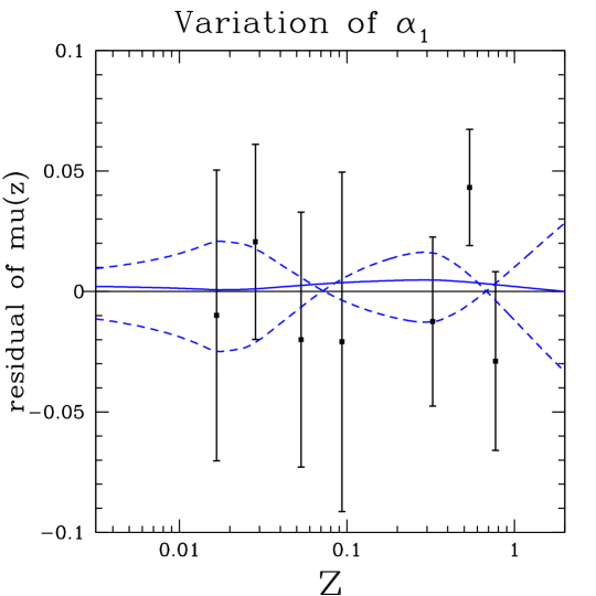
Residuals of the binned SNLS distance modulus data, after subtraction of the mean distance modulus for the $\Lambda$CDM model, are shown in Fig. 3. The binning is purely for plotting purposes. For calculation of the likelihood function we use the unbinned data.

2.2.5 Final Likelihood

We now have three independent data sets: CMB, BAO, and one of two supernova data sets. Since they are independent, the probabilities multiply:

$$\mathrm{ln}({\cal L}_{\rm TOT})=\mathrm{ln}(P_{CMB}(\omega_{m},D_{*}))-\frac{\chi^{2}_{SN}}{2}-\frac{\chi^{2}_{BAO}}{2},$$ (12)

where $\chi^{2}_{SN}$ comes from either the Gold or SNLS data set. Because the SNLS and Gold data sets make use of many of the same nearby supernovae, but use different algorithms for correcting the magnitudes, the data sets are correlated. Combining them appropriately would require more than a simple summing of the Fisher matrices and is an exercise we have not attempted.

2.3 Eigenmode Calculation

To select our modes we need the covariance matrix for the errors in the $\alpha_{i}$ parameters for some initial basis. One could in principle calculate the covariance matrix from an MCMC chain, but since a chain run with the full set of $\alpha_{i}$ parameters is highly non-Gaussian, the calculated covariance matrix is not a good approximation and does not give good eigenmodes. Instead we estimate it analytically from the Fisher matrix, and then use this estimate to define the modes.

2.3.1 The Fisher Matrix

First, we generate a Fisher matrix by expanding about a particular point. The point chosen is the mean point of a chain run with the aforementioned likelihood function, but using $\Omega_{\Lambda}$ instead of $\alpha_{i}$. This Fisher matrix is calculated in two parts. For the supernova part we obtain:

$$F^{SN}_{ij}=\sum_{k}\frac{\partial x_{k}}{\partial p_{i}}\frac{1}{\sigma_{k}^{2}}\frac{\partial x_{k}}{\partial p_{j}}$$ (13)

where for SNLS $p_{k}=(\omega_{m},\Omega_{k},M,\alpha,\beta,\alpha_{0},\alpha_{1},\alpha_{2},...,\alpha_{100})$ and

$$x_{k}\equiv 5\mathrm{log}_{10}\left(\frac{D_{L}(z_{k})}{10\mathrm{pc}}\right)+M-\alpha(s_{k}-1)+\beta c_{k}$$ (14)

and for Gold $p_{k}=(\omega_{m},\Omega_{k},\delta M,\alpha_{0},\alpha_{1},\alpha_{2},...,\alpha_{100})$ and

$$x_{k}\equiv 5\mathrm{log}_{10}\left(\frac{D_{L}(z_{k})}{10\mathrm{pc}}\right)+\delta M.$$ (15)

Since the BAO data are written as a single constraint in $A$, which is a function of the chain parameters, calculating its Fisher matrix is even simpler:

$$F^{BAO}_{ij}=\frac{\partial A}{\partial p_{i}}\frac{1}{\sigma^{2}}\frac{\partial A}{\partial p_{j}}.$$ (16)

Once this is calculated, we need to factor in the CMB data. Because performing numerical derivatives on our two-parameter probability matrix would be numerically unstable, we first calculate a covariance matrix from the chain calculated in section 2.2.1 which includes only $\omega_{m}$ and $D_{\ast}$, then invert this covariance matrix to obtain a Fisher matrix, which we will call $F^{2x2}$. We convert this Fisher matrix to one in the parameters of interest as follows:

$$F^{CMB}_{ij}=\left(\frac{\partial v}{\partial p_{i}}\right)^{T}F^{2x2}\left(\frac{\partial v}{\partial p_{j}}\right)$$ (17)

where $v$ is the vector defined by $v=\left[\omega_{m},D_{\ast}\right]$. Finally,

$$F_{ij}^{TOT}=F^{SN}_{ij}+F^{BAO}_{ij}+F^{CMB}_{ij}\mathrm{.}$$ (18)

This total Fisher matrix is then inverted to give us a covariance matrix for the eigenmode calculation. The covariance matrix, once diagonalized, gives us our eigenmodes.

2.3.2 Initial Basis and Diagonalization

Our specific goals for the desired modes are that there be one and only one constant mode, and that the time-varying modes have amplitudes with uncorrelated errors. We can meet these two criteria by careful selection of the initial basis and diagonalization procedure.

The initial basis must have the following properties:

1. It must have one element which is a constant.

2. The elements must be linearly independent.

Note that the second property is satisified by any basis by definition. There are many possible bases that satisfy these criteria. We have chosen ours with the additional (somewhat arbitrary) criteria that their dot products, $\sum_{a}e_{i}(z_{a})e_{j}(z_{a})=N\delta_{ij}$, where $N$ is the dimensionality of the space given by the discretization procedure. The normalization factor, $N$, keeps the shapes and amplitudes of the best-determined modes independent of $N$ as the continuum limit is approached. For completeness, we describe the initial basis in Appendix A.

Each basis element is defined based on its value at $N$ values of $z$ between 0 and 2. With the choice of uniform spacing in $\ln(0.01+z)$ we find we are able to approach the continuum limit with a smaller value of $N$ than with other possible choices, such as uniform spacing in $z$. The results in this paper were generated with $N=50$. Our basis is piecewise-linear in $\ln(0.01+z)$.

From the procedure in Appendix A we get $N$ $\alpha_{i}$ parameters with which to describe $\rho_{x}(z)$. To obtain our eigenmodes we invert the Fisher matrix in the parameter space of these $\alpha_{i}$ plus all our other parameters to obtain a covariance matrix. Then we take the $i>0$ subspace of this covariance matrix. Diagonalizing this $N-1$ by $N-1$ covariance matrix gives us our non-constant eigenmodes, each of which has errors uncorrelated with the other eigenmodes. Including the constant mode completes the space. We call this new basis $e^{\mathrm{em}}_{i}(z)$, and its coefficients $\alpha^{\mathrm{em}}_{i}$.

We typically truncate this new space by only keeping the first few best-measured eigenmodes. This results in an MCMC chain which is both highly Gaussian and easy to interpret, since a significant departure from zero of any one of the first few $\alpha^{em}_{i}$ parameters is a signature of non-constant dark energy. In the following we omit the superscript “em” from the $\alpha_{i}$ parameters to reduce notational clutter.

Note that the error in the constant mode has not been decorrelated with the errors in the non-constant modes. We discuss this choice in Appendix A.

2.4 Generating the Chain

We use the Metropolis-Hastings algorithm to generate a Monte Carlo Markov Chain (Gamerman, 1997) as described in Christensen et al. (2001). Due to the low computational requirements we are able to run very long chains with 6,010,000 elements. We then ignore the first 10,000 steps and thin the chain by taking every $20^{th}$ element, resulting in a chain of length 300,000.

We can be sure that this thinned, 300,000-length chain has converged by comparing the parameter estimates between different subsets of the chain. For example, if we take the subset of the first 5,000 elements of the thinned chain with $6$ dark energy parameters for the SNLS + CMB data set combination, and compare those parameter estimates to those of the last 5,000 elements of the chain, those parameter estimates usually vary by less than $\sigma/10$. Depending on the selection of elements, occasionally one of the 10 chain parameters will vary by as much as $\sigma/5$. Since the chain has converged to an accuracy within about $\sigma/10$ at the 90% confidence limit for each parameter after 5,000 elements, and we run the chain to 300,000, convergence is not an issue.

We use a generating function which is a multivariate normal distribution. Its covariance matrix is obtained from a pre-run. This pre-run is done in two iterations, each of length 100,000 with thinning by 20. The second iteration uses the covariance matrix from the first, with the covariance matrix from the second giving the covariance matrix used to run the final chain. This iterative process gives us a generating function that is a good Gaussian approximation to the full probability distribution. This match between generating function and posterior makes for an efficient exploration of the posterior.

We set a (weak) prior constraints on $\Omega_{m}$ by bounding it to the interval $0<\Omega_{m}<1$.

3 Results

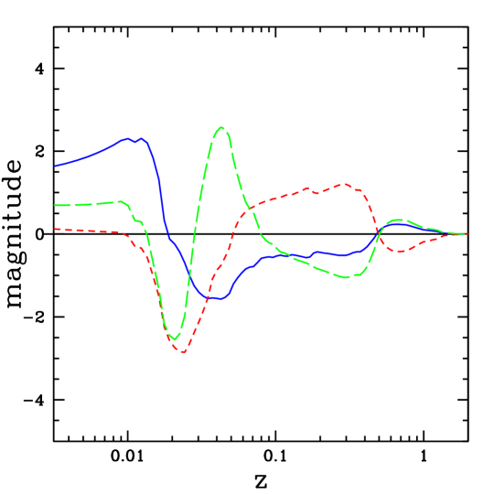
We start by examining one data set combination in detail: SNLS with CMB data. The first few eigenmodes are shown in figure 2. As is typical with such eigenmode decompositions, the frequency of oscillations tends to increase as the mode number increases.

The interpretation of these modes is simplified by examining them in the distance modulus space. The effect of varying $\alpha_{i}$ on distance modulus is complicated by the fact that $\alpha_{i}$ is correlated with $\omega_{m}$, $\Omega_{k}$, $\alpha_{0}$, and the supernova parameter $M$. Thus in Fig.  3 we take, for example, the parameter $\alpha_{1}$ in the center panel, and set it to its mean value plus $\sigma(\alpha_{1})$. We then examine the chain in a small region about this value to obtain the mean values for all of the other parameters in the chain and calculate $\mu(z)$ for this point in the parameter space. Finally, we subtract the best-fit $\Omega_{\Lambda}$ model for comparison. We also perform the same procedure at the mean value minus $\sigma(\alpha_{1})$ and then repeat for $\alpha_{0}$ and $\alpha_{2}$.

Figure 2: The three best-measured eigenmodes for the SNLS + CMB data set.

Figure 3: The observable consequences of altering the mode coefficients. The points with error bars are the binned SNLS residuals after subtraction of the mean $\Lambda$CDM distance modulus. The curves are the residual mean distance moduli with different constraints on $\alpha_{i}$ with $i=0$ (left panel), $i=1$ (center panel) and $i=2$ (right panel). The constraints are that $\alpha_{i}$ is held fixed at 1 $\sigma$ above or 1 $\sigma$ below its mean value (dashed curves). As the mode number is increased, the oscillation frequency increases.

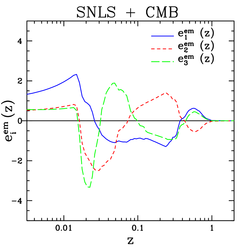
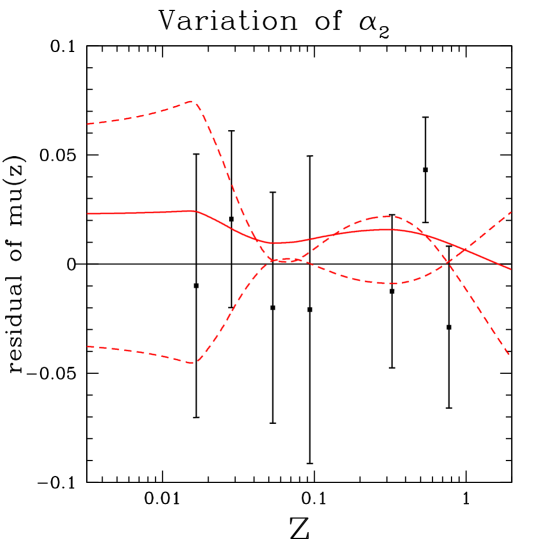
Note that these modes have significant support at $z<0.1$ and even $z<0.02$ and thus are affecting distances at redshifts as small as $0.02$. This is due to the nearby sample that spans $0.015<z<0.125$. The low-redshift support in these modes makes them potentially sensitive to large bulk flows (Shi, 1997; Shi & Turner, 1998; Zehavi et al., 1998) that systematically shift the redshifts of the observed supernovae from their Hubble flow values. Hui & Greene (2005) find surprising sensitivity of $w$ determinations to peculiar velocity effects in forecasts for future observations. Given the weight some of our best-determined modes place on low $z$ data, peculiar velocities could potentially be contributing significant systematic errors to our results as well. We address this concern below.

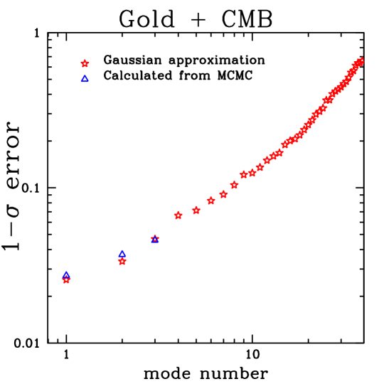
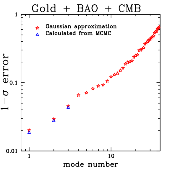
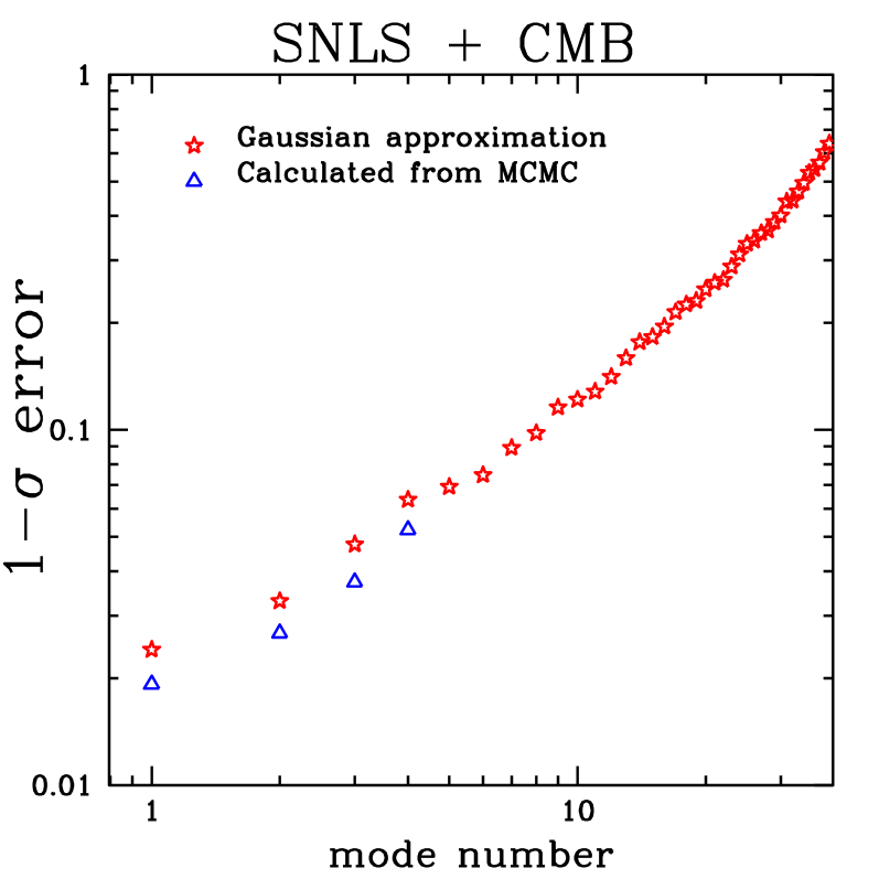
The whole spectrum of (square roots of) eigenvalues for these modes is shown in Fig. 4. The stars are the result of our Fisher matrix calculation and the triangles from MCMC. Including more than four modes in our MCMC calculation leads to gross degeneracies that do not occur in the Gaussian approximation; we have not been able to reliably calculate the spectrum beyond this first handful of modes. For these lowest modes we see the Gaussian approximation provides a description of the errors good to about 15%. For the Gold data (see Appendix B) the Gaussian approximation is even better.

At first blush, the large number of low noise modes contradicts what we know about the eigenvalue spectrum of $w(z)$. Knox et al. (2005) found that for a future space-based mission only a few $w(z)$ modes could be reconstructed with errors smaller than 0.1. Here, for current data, we see eight time-varying $\rho_{x}(z)/\rho_{c}$ modes can be reconstructed with errors smaller than 0.1. Others have pointed out that $\rho_{x}(z)$ can be reconstructed with much smaller fractional errors than $w(z)$ (Wang & Freese, 2006). It is well known that differentiating data makes them noisier and, roughly speaking, reconstructing $w(z)$ requires one more differentiation of the data than a reconstruction of $\rho_{x}(z)$.

We only mean to point out here that there is this difference, and that the reasons for it can be understood. We are not using this difference as an argument that one should consider only $\rho_{x}(z)$ and not $w(z)$. Although $w(z)$ has larger error bars than $\rho_{x}(z)/\rho_{c}$, this is not because more information is lost in a reduction to $w(z)$. There is a $\rho_{x}(z)$ for every $w(z)$, obtainable by integration. What happens in integrating noisy modes of $w(z)$ to get the corresponding $\rho_{x}(z)$ is that the rapid oscillations with larger departures from the fiducial value of -1 get averaged out, suppressing the rapid oscillations. A large amplitude (compared to fiducial value of -1) noise fluctuation on a $w(z)$ mode will be a much smaller fluctuation on the corresponding $\rho_{x}(z)$ (compared to fiducial value of $\Omega_{x}\rho_{c}$). For discussion of the relative merits of parameterizing dark energy by $\rho_{x}(z)$ and $w(z)$ see Linder (2004).

Figure 4: The one $\sigma$ errors for the first 40 of our 50 eigenmode amplitudes plotted for both the MCMC analysis and the Fisher matrix analysis for SNLS + CMB. The $1-\sigma$ errors from the Fisher matrix are the square roots of the eigenvalues of the inverse of the Fisher matrix associated with the respective modes. The modes are normalized to have length $\sqrt{N}$ where $N$ is the number of basis elements, as described in 2.3.2.

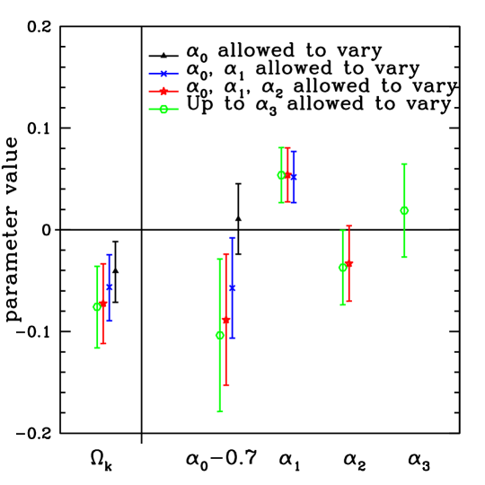
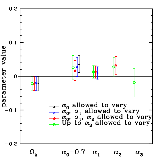
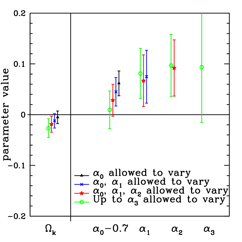
In figure 5 we plot our estimates of $\Omega_{k}$, $\alpha_{0}-0.7$, and some of the varying $\alpha_{i}$ parameters. We subtract $0.7$ from $\alpha_{0}$ for plotting convenience. Recall that $\Omega_{\Lambda}=\alpha_{0}$ when the time-varying modes have zero amplitude. The multiple data points for a given parameter are the results for different numbers of parameters held fixed.

Figure 5: Parameter estimates for the SNLS + CMB data set. For each parameter, we estimated the value multiple times, each time allowing a different number of dark energy parameters to vary.

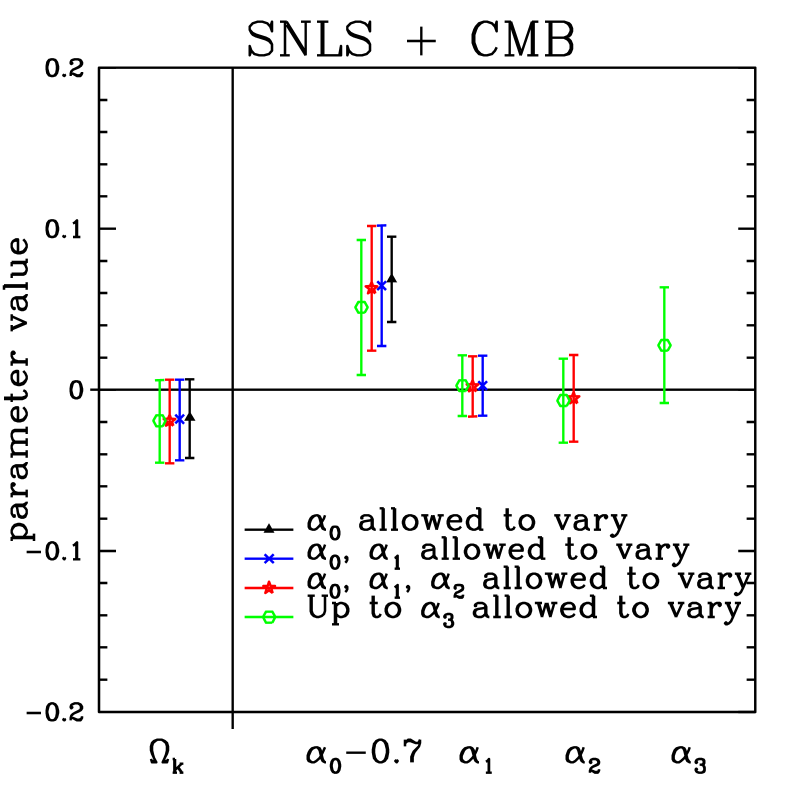
Note that the first three nonconstant mode amplitudes are consistent with zero. Like many others (Doran et al., 2005; Daly & Djorgovski, 2005; Xia et al., 2005; Ichikawa & Takahashi, 2005; Sánchez et al., 2006; Nesseris & Perivolaropoulos, 2005) we are finding consistency of available supernova plus CMB data with a flat $\Lambda$CDM universe.

Note also that the curvature constraints are robust to variation of these first few modes. They are sufficiently well-constrained that they do not lead to significant confusion with the curvature.

We also see that the amplitudes of the nonconstant eigenmodes themselves do not change appreciably when we change how many mode amplitudes we vary. Within the Gaussian approximation this independence is expected, since the modes were chosen to have uncorrelated Fisher matrix amplitude errors.

While we have shown that for the first few dark energy parameters our Gaussian approximation remains valid and the curvature constraint remains robust, we expect that if we add more and more dark energy parameters, eventually these facts will change. We expect this for two reasons. First, the freedom to vary the more poorly constrainted parameters will allow us to move far enough away in parameter space (from the point at which the Fisher matrix was evaluated) for the Gaussian approximation to break down. Second, even within the Gaussian approximation, the errors in the amplitudes of the dark energy modes are only constructed to be uncorrelated with each other; they are correlated with the errors in all of the other parameters, including the displayed $\Omega_{k}$ and $\alpha_{0}$. Thus including more modes will weaken these constraints. In figure 6 we see the results of including up to mode number 6.

Figure 6: As we allow more freedom in $\rho_{x}(z)$ by allowing more $\alpha_{i}$ to vary, the errors in the inferred cosmological parameters grow. The leftmost estimate for each parameter comes from a chain allowing up to $\alpha_{6}$ to vary. For $\alpha_{0}-0.7$ this left-most estimate is off the chart.

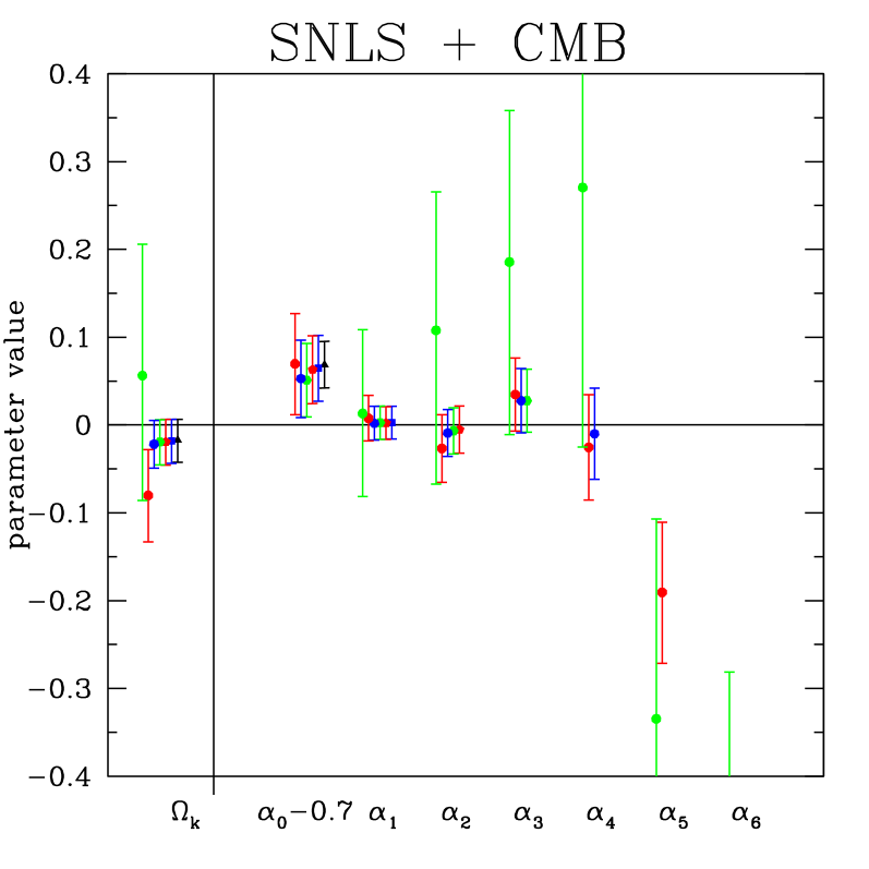
The breakdown of Gaussianity is very sudden. The moment the chain includes the parameter $\alpha_{6}$, the errors on all other parameters increase dramatically. We believe the breakdown is driven by a correlation between the $\alpha_{6}$ error and the $\alpha_{0}$ error, which then allows for variations far from the fiducial model. With these large variations the mean values of our cosmological parameters end up describing a cosmology that is inconsistent with other experiments. For example, when we include the $\alpha_{6}$ parameter, $\Omega_{m}$ gets dragged up against the prior’s upper bound of 1 so that $\Omega_{m}=0.89+0.10-0.27$ at 95% confidence.

Results from the other data set combinations are not dramatically different to those from SNLS plus CMB that we have considered here in detail. For completeness, we include them in Appendix B.

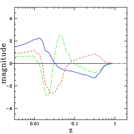
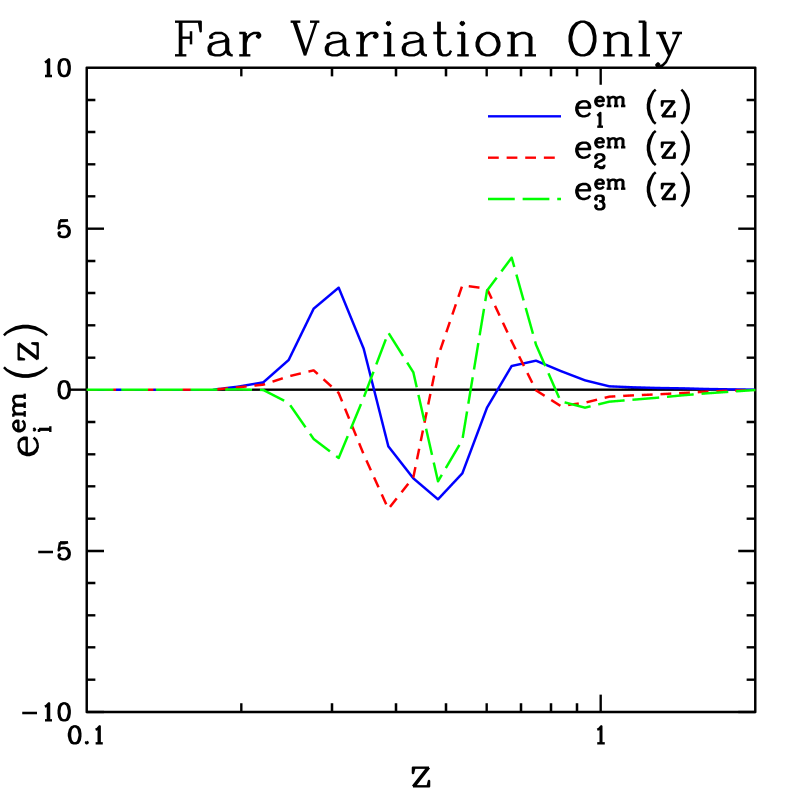
We now turn to the concern that because our best-determined modes have strong support at very low redshift they may be contaminated by (unmodeled) peculiar velocity-induced redshifts. We address it by constructing modes (as described in Appendix A) that only have variation in the region 0.2 ¡ z ¡ 2.0. This region contains all the SNLS supernovae and none of the supernovae from the nearby sample.

Our best-determined modes resulting from this procedure are shown in Fig. 7 and the corresponding parameter constraints are shown in Fig. 8. These mode amplitudes have larger error bars than the previous ones, but are safer from contamination by peculiar velocities.

Figure 7: The three best-measured eigenmodes for the SNLS + CMB data set with the restriction that the modes only vary at $z>0.2$.

Figure 8: Parameter estimates for the SNLS + CMB data set with the time-varying dark energy modes as shown in Fig. 7. For each parameter, we estimated the value multiple times, each time allowing a different number of dark energy parameters to vary.

4 Discussion

Our modes have been defined based on which ones can be best determined by the data. We now turn to consideration of the expected signal contribution to these mode amplitudes.

It is difficult to see how the dark energy density could vary on time scales faster than a Hubble time. Were the dark energy density to start diluting with the expansion as $a^{n}$ we would have $d\ln\rho/dt=nH$; i.e. the time-scale for variation would be $1/|nH|$. Even were the dark energy density to suddenly thermalize as massless radiation we would only have $n=-4$. Expressing $n$ in terms of variation of the equation-of-state parameter away from its value for a cosmological constant ($\delta w=w-(-1)$) we have $n=3\delta w$. Thus we roughly expect $|d\ln\rho/dt|<H$.

Ignoring contributions to $H$ from curvature and matter, we can write $d\ln\rho_{x}/dt/H=d\rho_{x}/\rho_{x}/da/a$ which can be conveniently calculated for our modes by finite difference. Note that the time-scale for variation is not a property of the mode itself, but a property of the mode and the amplitude of the mode. We evaluate it for each mode with an amplitude equal to its $1\sigma$ uncertainty. We find they all have regions of redshift for which they exceed unity, as can be seen in the two panels of Fig. 9.

Figure 9: $(\Delta\rho_{x}/\rho_{x})/(\Delta a/a)$ for our modes with amplitudes at their 68% confidence upper limits. This is roughly equal to the ratio of the natural time-scale for variation ($1/H$) to the mode variation time-scale $(d\ln\rho/dt)^{-1}$. We see that the mode variation time-scales are longer than the natural time scale. Top panel: modes varying over all $z$. Bottom panel: modes varying only in the SNLS region.

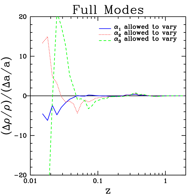
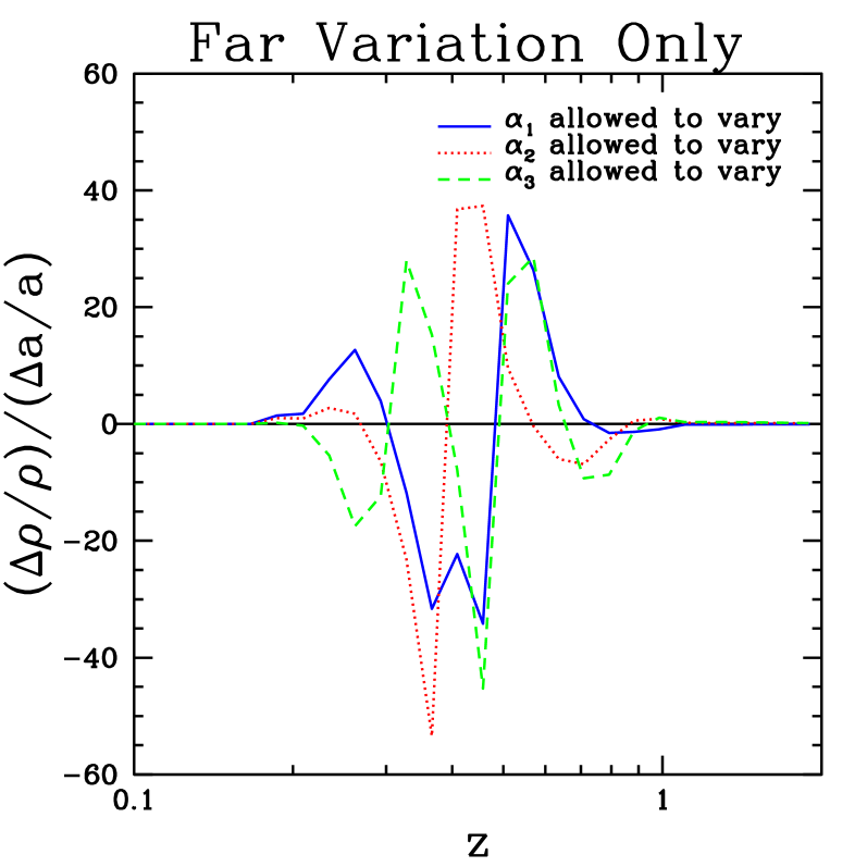
Note that even though the far region modes in Fig. 7 look smoother than those in Fig. 2, their amplitude constraints are weaker with the result that the density variation time scales, evaluated with an amplitude of $1\sigma$, are actually smaller than those for the full modes.

We have also explored the idea of finding modes that maximize signal-to-noise ratio rather than the ones that merely minimize noise. We have attempted to do so using the technique of signal-to-noise eigenmodes Bond (1995); Bunn & Sugiyama (1995); Karhunen (1947), also known as the Karhunen-Loeve technique.

The procedure in general is for data with both a noise covariance matrix and a signal covariance matrix; i.e., data that is modeled as

$$\Delta_{i}=s_{i}+n_{i}$$ (19)

where the signal contribution has covariance matrix

$$S_{ij}=\langle\left(s_{i}-\langle s_{i}\rangle\right)\left(s_{j}-\langle s_{j}\rangle\right)\rangle$$ (20)

and similarly for the noise, $N_{ij}\equiv\langle n_{i}n_{j}\rangle$.

The procedure starts with a whitening of the data so that all modes have errors that are uncorrelated with unit variance. The signal matrix in this new space is $N^{-1/2}SN^{-1/2}$. Eigenmodes of this ‘signal-to-noise matrix’ have eigenvalues that are equal to the signal-to-noise ratio which is exactly what we want.

For our application we view the density in redshift bins as the ‘data’. The trick is identifying a useful form of the signal matrix. To date we have not found a useful form. For the signal matrices which we have tried, the result has been that though the modes themselves become smoother, the error estimates increase, such that the density variation time scale, evaluated with an amplitude of $1\sigma$, does not decrease substantially.

5 Conclusions

The single most important question about the dark energy is whether it is a cosmological constant. We have presented a method to test this hypothesis by looking for the deviations from constant density that are easiest to detect. The best-determined time-varying modes of $\rho_{x}(z)$ are found by use of a Gaussian approximation to the parameter likelihood, but the estimates of the amplitudes of these modes do not use the Gaussian approximation. We have applied the method to supernova, CMB and BAO data.

We found that SNLS + CMB data are capable of constraining the amplitudes of three time-varying modes of $\rho_{x}(z)$ to better than 5%. None of them are significantly different from zero. We found that if only these well-constrained modes are allowed to vary then the curvature is also not significantly different from zero. We found that the best-determined mode amplitudes have highly independent errors, which within the Gaussian approximation occurs by design. We found that they are sensitive to density variations at very low ($z\sim 0.02$) redshifts. We noted that these redshifts are sufficiently small to raise concerns about the effects of bulk flows. We pointed out that the best-determined modes are useful not only for detection of time variation, but also for ferreting out systematic errors by studying how the amplitude estimates fluctuate with varying data subsample.

We pointed out that, by quite general considerations of the time-scales expected for dark energy density variation, at the achieved sensitivity levels we do not expect a detectable signal. Because we strongly expect a null result, our application can be viewed as a consistency test which has the potential for exposing systematic errors. This situation is analogous to that with the (theoretially unexpected) B-modes which are a useful diagnostic in cosmic shear observations (e.g. Crittenden et al., 2002). As the statistical constraining power of the data improves we will begin to probe the regime where signals can be expected. We also suggested that with the adoption of an appropriate signal covariance matrix we could use the signal-to-noise eigenmode technique to maximize signal-to-noise ratio rather than simply minimizing noise.

In Appendix B our results show that the BAO data add significant additional constraining power to our cosmological parameter estimates. Unfortunately, the convenient reduction to a single number, though valuable for other applications where the dark energy is assumed to have a constant equation-of-state parameter, is not clearly applicable to our problem. It would be useful to have a reduction of the BAO data to constraints on the distances to several redshifts, or as a single constraint on some linear combination of redshifts.

A Pre-diagonalization modes

Here we describe our construction of the initial basis that we use as the first step in creating the time-varying modes with uncorrelated amplitude errors.

The first basis vector is a constant, which before normalization looks like (1, 1, 1, … , 1). The next $\frac{N}{2}$ basis vectors take the form (0, 0, 1, -1, 0, …, 0). As long as none of the non-zero values in this second set of basis vectors overlap with one another, they will be orthogonal to one another, and each is clearly orthogonal to the constant vector.

To fill out the space further with a third set of basis vectors we notice that each of the second set of basis vectors is orthogonal to the constant vector, but only in steps of two. A new basis vector that maintains the same value in steps of two will be orthogonal to each previous basis vector: (1, 1, -1, -1, 0, …, 0). To find the next one we consider that this basis vector is orthogonal to (1, 1, 1, 1, 0, …, 0), so with the previous argument all the basis vectors made so far will clearly be orthogonal to (1, 1, 1, 1, -2, -2, 0, …, 0). The next basis vector will then include 6 1’s and two -3’s, and so on. Careful counting reveals that there are $\frac{N}{2}-1$ of this third set of basis vectors, which will complete our basis if we have an even number of elements. If we have an odd number of elements we can add a final basis vector that takes the form (1, 1, 1, …, 1, -(n-1)), since every element of the second set of basis vectors contains a zero in the last position.

Below is an example $9\times 9$ basis (with vectors as rows), before normalization.

$$\begin{array}[]{rrrrrrrrr}1&1&1&1&1&1&1&1&1\\ 1&-1&0&0&0&0&0&0&0\\ 0&0&1&-1&0&0&0&0&0\\ 0&0&0&0&1&-1&0&0&0\\ 0&0&0&0&0&0&1&-1&0\\ 1&1&-1&-1&0&0&0&0&0\\ 1&1&1&1&-2&-2&0&0&0\\ 1&1&1&1&1&1&-3&-3&0\\ 1&1&1&1&1&1&1&1&-8\\ \end{array}$$ (A1)

Each of these basis vectors defines an $e^{0}_{i}(z)$. To do this, we connect each element in the vector with a particular position in $z$. The value of $e^{0}_{i}(z)$ between these positions is given by linear interpolation. These basis vectors $e^{0}_{i}(z)$ are used to define $\rho_{x}(z)$ as in equation (A2):

$$\rho_{x}(z)=\rho_{c}(z=0)\sum_{i=0}^{N}\alpha^{0}_{i}e^{0}_{i}(z).$$ (A2)

It is worth noting that while we demanded that the non-constant eigenmodes were also zero-mean, there is an arbitrariness to the meaning of zero mean. It depends on the definition of the dot product, which is, in turn, basis-dependent. For example, the average value of a mode sampled in $\ln(z)$ is different from the average value of the same mode sampled in $z$.

Given this arbitrariness, it is worth considering relaxing the zero-mean condition. With that condition abandoned, it becomes possible to use the new freedom to decorrelate the time-varying mode amplitude errors with the constant mode amplitude error. In principle one could do so in two steps: first add the right amount of constant to each of our time-varying modes to decorrelate it with the constant. Then re-diagonalize in the time-varying subspace. In practice we have been unable to circumvent numerical instabilities that occur when we attempt this procedure.

In order to suppress variation of the near region, we chose to modify our pre-diagonalization basis. We select a basis where the first mode is a constant. The second is constant over the near region and the far region, with the two differring in sign, with the values of the near and far regions chosen to enforce orthogonality with the constant mode. The next group of modes varies only in the near region, with the far region set to zero. Its structure is the same as that described earlier for the varying basis elements. The final group of modes again has the same structure, but varies only in the far region. An example $9\times 9$ basis is shown below (before normalization).

$$\begin{array}[]{rrrrrrrrr}1&1&1&1&1&1&1&1&1\\ 5&5&5&5&-4&-4&-4&-4&-4\\ 1&-1&0&0&0&0&0&0&0\\ 0&0&1&-1&0&0&0&0&0\\ 1&1&-1&-1&0&0&0&0&0\\ 0&0&0&0&1&-1&0&0&0\\ 0&0&0&0&0&0&1&-1&0\\ 0&0&0&0&1&1&-1&-1&0\\ 0&0&0&0&1&1&1&1&-4\\ \end{array}$$ (A3)

The location of the split is chosen to coincide with the desired location before which no variation will occur. Once this basis is chosen, we carry out the diagonalization procedure as described in 2.3.2, with the exception that we choose the subset of the covariance matrix that corresponds to those basis elements which only vary in the far region.

B Other Data Combinations

Here we show results from application to other data combinations and comment on the difficulty of including the BAO data. The results from the various other data set combinations we calculated are shown in figures 10, 11 and 12.

Figure 10: Eigenmodes (left panel), Eigenvalue spectrum (center panel) and parameter estimates (right panel) for BAO plus SNLS plus CMB data.

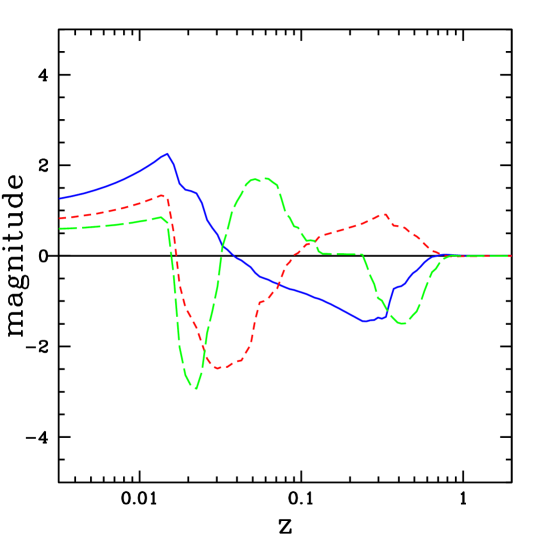
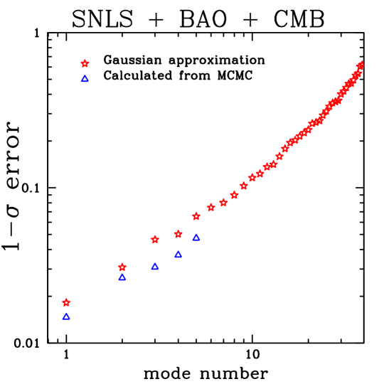
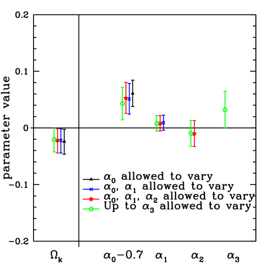
Adding in the BAO data, we find that we gain a fair amount of extra constraining power for both curvature and our dark energy parameters. For the SNLS data adding in the BAO data gives us the ability to measure one more dark energy parameter. Interpretation of these results though is severely hampered by the manner in which we incorporated the BAO data. As described in the text we utilized the Eisenstein et al. (2005) reduction of their data to a constraint on a combination of $D_{M}(z)$ and $H(z)$ at $z=0.35$ and the matter density (their $A$ parameter). Although they tested the validity of this data compression for constant $w$ models, we are not sure how valid it is for the more general dark-energy model space that we consider. We include the BAO data only to show the potential statistical power of that data for an analysis such as ours.

Artifacts of the compression to $A$ could be seen in the modes had we not employed the following trick: when calculating the Fisher matrix in order to get the modes, we held the $H(z)$ in $A$ fixed. If we were to include $\partial H(z)/\partial\alpha_{i}$ as a contribution to $\partial A/\partial\alpha_{i}$ then there would be a large spike in the modes at $z=0.35$. This change to the eigenmodes makes no measurable difference to the parameter estimates.

Figure 11: As above, but for the Gold supernova data set combined with the CMB.

Figure 12: As above, but for the Gold supernova data set combined with BAO plus CMB.

References

- Astier et al. (2005) Astier, P., Guy, J., Regnault, N., Pain, R., Aubourg, E., Balam, D., Basa, S., Carlberg, R. G., Fabbro, S., Fouchez, D., Hook, I. M., Howell, D. A., Lafoux, H., Neill, J. D., Palanque-Delabrouille, N., Perrett, K., Pritchet, C. J., Rich, J., Sullivan, M., Taillet, R., Aldering, G., Antilogus, P., Arsenijevic, V., Balland, C., Baumont, S., Bronder, J., Courtois, H., Ellis, R. S., Filiol, M., Goncalves, A. C., Goobar, A., Guide, D., Hardin, D., Lusset, V., Lidman, C., McMahon, R., Mouchet, M., Mourao, A., Perlmutter, S., Ripoche, P., Tao, C., & Walton, N. 2005, ArXiv Astrophysics e-prints
- Bernstein (2005) Bernstein, G. 2005, ArXiv Astrophysics e-prints
- Bond (1995) Bond, J. R. 1995, Phys. Rev. Lett., 74, 4369
- Bunn & Sugiyama (1995) Bunn, E. F. & Sugiyama, N. 1995, ApJ, 446, 49
- Chevallier & Polarski (2001) Chevallier, M. & Polarski, D. 2001, International Journal of Modern Physics D, 10, 213
- Christensen et al. (2001) Christensen, N., Meyer, R., Knox, L., & Luey, B. 2001, Classical Quantum Gravity, 18, 2677
- Chu et al. (2005) Chu, M., Eriksen, H. K., Knox, L., Górski, K. M., Jewell, J. B., Larson, D. L., O’Dwyer, I. J., & Wandelt, B. D. 2005, Phys. Rev. D, 71, 103002
- Crittenden et al. (2002) Crittenden, R. G., Natarajan, P., Pen, U.-L., & Theuns, T. 2002, ApJ, 568, 20
- Daly & Djorgovski (2004) Daly, R. A. & Djorgovski, S. G. 2004, ApJ, 612, 652
- Daly & Djorgovski (2005) —. 2005, American Astronomical Society Meeting Abstracts, 207,
- Doran et al. (2005) Doran, M., Karwan, K., & Wetterich, C. 2005, Journal of Cosmology and Astro-Particle Physics, 11, 7
- Eisenstein et al. (2005) Eisenstein, D. J., Zehavi, I., Hogg, D. W., Scoccimarro, R., Blanton, M. R., Nichol, R. C., Scranton, R., Seo, H.-J., Tegmark, M., Zheng, Z., Anderson, S. F., Annis, J., Bahcall, N., Brinkmann, J., Burles, S., Castander, F. J., Connolly, A., Csabai, I., Doi, M., Fukugita, M., Frieman, J. A., Glazebrook, K., Gunn, J. E., Hendry, J. S., Hennessy, G., Ivezić, Z., Kent, S., Knapp, G. R., Lin, H., Loh, Y.-S., Lupton, R. H., Margon, B., McKay, T. A., Meiksin, A., Munn, J. A., Pope, A., Richmond, M. W., Schlegel, D., Schneider, D. P., Shimasaku, K., Stoughton, C., Strauss, M. A., SubbaRao, M., Szalay, A. S., Szapudi, I., Tucker, D. L., Yanny, B., & York, D. G. 2005, ApJ, 633, 560
- Freivogel et al. (2005) Freivogel, B., Kleban, M., Rodriguez Martinez, M., & Susskind, L. 2005, ArXiv High Energy Physics - Theory e-prints
- Gamerman (1997) Gamerman, D. 1997, Markov Chain Monte Carlo: stochastic simulation for Bayesian inference (Chapman and Hall)
- Hu & Dodelson (2002) Hu, W. & Dodelson, S. 2002, ARA&A, 40, 171
- Hui & Greene (2005) Hui, L. & Greene, P. B. 2005, ArXiv Astrophysics e-prints
- Huterer & Cooray (2005) Huterer, D. & Cooray, A. 2005, Phys. Rev. D, 71, 023506
- Huterer & Starkman (2003) Huterer, D. & Starkman, G. 2003, Physical Review Letters, 90, 31301
- Ichikawa & Takahashi (2005) Ichikawa, K. & Takahashi, T. 2005, ArXiv Astrophysics e-prints
- Jones et al. (2005) Jones, W. C. et al. 2005, ArXiv Astrophysics e-prints
- Karhunen (1947) Karhunen, K. 1947, Uber lineare Methoden in der Wahrscheinlichkeitsrechnung (Kirjapaino oy. sana, Helsinki)
- Knox (2006) Knox, L. 2006, Phys. Rev. D, 73, 023503
- Knox et al. (2005) Knox, L., Albrecht, A., & Song, Y. S. 2005, in ASP Conf. Ser. 339: Observing Dark Energy, 107–+
- Linder (2003) Linder, E. V. 2003, Physical Review Letters, 90, 091301
- Linder (2004) —. 2004, Phys. Rev. D, 70, 061302
- Linder (2005) —. 2005, Astroparticle Physics, 24, 391
- Linder & Huterer (2005) Linder, E. V. & Huterer, D. 2005, ArXiv Astrophysics e-prints
- MacTavish et al. (2005) MacTavish, C. J. et al. 2005, ArXiv Astrophysics e-prints
- Montroy et al. (2005) Montroy, T. E. et al. 2005, ArXiv Astrophysics e-prints
- Nesseris & Perivolaropoulos (2005) Nesseris, S. & Perivolaropoulos, L. 2005, Phys. Rev. D, 72, 123519
- Piacentini et al. (2005) Piacentini, F. et al. 2005, ArXiv Astrophysics e-prints
- Readhead et al. (2004a) Readhead, A. C. S., Mason, B. S., Contaldi, C. R., Pearson, T. J., Bond, J. R., Myers, S. T., Padin, S., Sievers, J. L., Cartwright, J. K., Shepherd, M. C., Pogosyan, D., Prunet, S., Altamirano, P., Bustos, R., Bronfman, L., Casassus, S., Holzapfel, W. L., May, J., Pen, U.-L., Torres, S., & Udomprasert, P. S. 2004a, ApJ, 609, 498
- Readhead et al. (2004b) Readhead, A. C. S., Myers, S. T., Pearson, T. J., Sievers, J. L., Mason, B. S., Contaldi, C. R., Bond, J. R., Bustos, R., Altamirano, P., Achermann, C., Bronfman, L., Carlstrom, J. E., Cartwright, J. K., Casassus, S., Dickinson, C., Holzapfel, W. L., Kovac, J. M., Leitch, E. M., May, J., Padin, S., Pogosyan, D., Pospieszalski, M., Pryke, C., Reeves, R., Shepherd, M. C., & Torres, S. 2004b, Science, 306, 836
- Riess et al. (2004) Riess, A. G., Strolger, L., Tonry, J., Casertano, S., Ferguson, H. C., Mobasher, B., Challis, P., Filippenko, A. V., Jha, S., Li, W., Chornock, R., Kirshner, R. P., Leibundgut, B., Dickinson, M., Livio, M., Giavalisco, M., Steidel, C. C., Benítez, T., & Tsvetanov, Z. 2004, ApJ, 607, 665
- Sánchez et al. (2006) Sánchez, A. G., Baugh, C. M., Percival, W. J., Peacock, J. A., Padilla, N. D., Cole, S., Frenk, C. S., & Norberg, P. 2006, MNRAS, 366, 189
- Shapiro & Turner (2005) Shapiro, C. & Turner, M. S. 2005, ArXiv Astrophysics e-prints
- Shi (1997) Shi, X. 1997, ApJ, 486, 32
- Shi & Turner (1998) Shi, X. & Turner, M. S. 1998, ApJ, 493, 519
- Sievers et al. (2005) Sievers, J. L. et al. 2005, ArXiv Astrophysics e-prints
- Simpson & Bridle (2006) Simpson, F. & Bridle, S. 2006, ArXiv Astrophysics e-prints
- Song & Knox (2004) Song, Y. & Knox, L. 2004, Phys. Rev. D, 70, 063510
- Spergel et al. (2006) Spergel, D. N., Bean, R., Dore’, O., Nolta, M. R., Bennett, C. L., Hinshaw, G., Jarosik, N., Komatsu, E., Page, L., Peiris, H. V., Verde, L., Barnes, C., Halpern, M., Hill, R. S., Kogut, A., Limon, M., Meyer, S. S., Odegard, N., Tucker, G. S., Weiland, J. L., Wollack, E., & Wright, E. L. 2006, ArXiv Astrophysics e-prints
- Spergel et al. (2003) Spergel, D. N., Verde, L., Peiris, H. V., Komatsu, E., Nolta, M. R., Bennett, C. L., Halpern, M., Hinshaw, G., Jarosik, N., Kogut, A., Limon, M., Meyer, S. S., Page, L., Tucker, G. S., Weiland, J. L., Wollack, E., & Wright, E. L. 2003, ApJS, 148, 175
- Wang & Freese (2006) Wang, Y. & Freese, K. 2006, Physics Letters B, 632, 449
- Wang & Tegmark (2004) Wang, Y. & Tegmark, M. 2004, Physical Review Letters, 92, 241302
- Wang & Tegmark (2005) —. 2005, Phys. Rev. D, 71, 103513
- Weller & Albrecht (2002) Weller, J. & Albrecht, A. 2002, Phys. Rev. D, 65, 103512
- Xia et al. (2005) Xia, J.-Q., Zhao, G.-B., Feng, B., Li, H., & Zhang, X. 2005, ArXiv Astrophysics e-prints
- Zehavi et al. (1998) Zehavi, I., Riess, A. G., Kirshner, R. P., & Dekel, A. 1998, ApJ, 503, 483