Placing Confidence Limits on Polarization Measurements

Abstract

The determination of the true source polarization given a set of measurements is complicated by the requirement that the polarization always be positive. This positive bias also hinders construction of upper limits, uncertainties, and confidence regions, especially at low signal-to-noise levels. We generate the likelihood function for linear polarization measurements and use it to create confidence regions and upper limits. This is accomplished by integrating the likelihood function over the true polarization (parameter space), rather than the measured polarization (data space). These regions are valid for both low and high signal-to-noise measurements.

1 Introduction

Measurements of linear polarization generally provide values for the degree and angle of polarization. They may also provide upper limits on the degree of polarization even where the nominal values $P$ are not much larger than the uncertainties $\sigma$ (i.e. at low signal-to-noise). Polarization maps typically plot vectors in regions where measurements are made with high confidence and open circles where the polarization is found to be too low to justify a vector, but where useful upper limits can still be estimated (e.g. where $P+2\sigma<1\%$; Dotson et al. 2000).

While the distributions of the polarization degree and angle are not normal (gaussian), it is still possible to place estimates and uncertainties and confidence levels on their values. The position angle distribution, while non-normal, is symmetric about the measured angle so that estimates and uncertainties on its value are fairly straightforward (Naghizadeh-Khouei & Clarke, 1993). Estimates of the polarization degree are complicated by the fact that it must always be positive, introducing a bias into any estimate. For any true polarization degree $P_{0}$, we expect on average to measure a polarization degree $P>P_{0}$. This problem has been thoroughly investigated by Simmons & Stewart (1985; hereafter SS85).

SS85 have also devised a procedure to place uncertainties on the polarization degree. First, the expected probability density of polarization (§2) is integrated over a set of possible measurements. However, this only places limits on the measured polarization $P$, the limits varying with the value of the true polarization $P_{0}$. To correct for this and thus create confidence limits on the parameter $P_{0}$, SS85 project their results onto the $P_{0}$-axis.

Here we introduce a slightly different procedure for determining confidence regions on the true polarization. Rather than integrate the probability density function over the data-space of the measured polarization, we integrate over the parameter-space of the true polarization. In this way we directly determine the likelihood (§3) that a measured polarization $P$ was drawn from a source of true polarization $P_{0}$.

2 Rice Distribution

Measuring the degree and angle of polarization is equivalent to determining of the amplitude and phase of a sinusoidal signal in the presence of noise. The joint and marginal probability distribution functions for the amplitude and phase have been discussed in detail by other authors (Rice, 1945; Vinokur, 1965; Simmons & Stewart, 1985). For completeness we review their results here.

Consider the simple case of rotating a linear polarizer through some angle $\theta$. The resulting signal changes as

$$S(\theta)=P\cos 2(\theta+\phi)+S_{N},$$ (1)

where the amplitude $P$ is the polarization degree, $\phi$ a relative phase shift (the polarization angle), and $S_{N}$ gaussian random noise. This form can be decomposed into two orthogonal components

$$S(\theta)=(q+q_{N})\cos 2\theta-(u+u_{N})\sin 2\theta,$$ (2)

where

$$q = P\cos 2\phi,$$ (3)

$$u = P\sin 2\phi,$$ (4)

$q_{N}$ is the noise component in phase with $\cos 2\theta$ and $u_{N}$ is the noise component in phase with $\sin 2\theta$. In optics $q$ and $u$ are known as Stokes parameters. In electronics they are often referred to as the “in-phase” and “quadrature-phase” components, respectively.

Since $S_{N}$ is gaussian, the measured Stokes parameters $q$ and $u$ are normally distributed about the true values $q_{0}$ and $u_{0}$ with equal uncertainties $\sigma$ (i.e. $\langle q_{N}^{2}\rangle=\langle u_{N}^{2}\rangle=\sigma$). The values of $q_{0}$ and $u_{0}$ are given by equations (3) and (4), replacing $P$ by $P_{0}$ and $\phi$ by $\phi_{0}$. The uncertainty in the polarization $P$ is also given by $\sigma$.

The joint probability distribution for $q$ and $u$ is given by the product of their individual normal distributions. Transforming to the polar coordinates $P$ and $\phi$ yields

$$f(P,\phi)=\frac{1}{2\pi\sigma^{2}}\exp\left[-\frac{P^{2}+P_{0}^{2}-2PP_{0}\cos 2(\phi-\phi_{0})}{2\sigma^{2}}\right].$$ (5)

The probability of measuring a polarization in the range [$P$, $P+\mathrm{d}P$] and [$\phi$, $\phi+\mathrm{d}\phi$] is given by $f(P,\phi)\,P\,\mathrm{d}P\,\mathrm{d}(\phi-\phi_{0})$. Integrating over $\mathrm{d}(\phi-\phi_{0})$ yields the Rice distribution for the polarization degree:

$$F(P|P_{0})\,\mathrm{d}P = \frac{1}{2}P\,\mathrm{d}P\int\limits_{-\pi/2}^{\pi/2}f(P,\phi)\,\mathrm{d}(\phi-\phi_{0})$$ (6)

$$= \frac{P}{\sigma}\exp\left[-\frac{P^{2}+P_{0}^{2}}{2\sigma^{2}}\right]I_{0}\left(\frac{PP_{0}}{\sigma^{2}}\right)\frac{\mathrm{d}P}{\sigma},$$

where $I_{0}()$ is the zeroth order modified Bessel function. (The pre-factor of $\text@frac{1}{2}$ in the integral of eq. [6] corrects for the $\pi$-periodicity of $\phi$.)

The asymmetry of this distribution with respect to $P$ and $P_{0}$ (evident in Fig. 1 for low values of $P_{0}/\sigma$) results in the positive bias of the measured polarization. For high signal-to-noise the Rice distribution is near-normal with mean approaching $P_{0}$ and a standard deviation approaching $\sigma$ (e.g. Rice 1945).

Figure 1: Probability density distribution for the measured polarization $P/\sigma$, given by equation (6). Distributions are shown for several different values of the true polarization $P_{0}/\sigma$.

3 The Likelihood Function

3.1 Constructing the Polarization Likelihood

If the true polarization $P_{0}$ is known, the probability that a measurement will be made in the range [$P$, $P+\mathrm{d}P$], is given by equation (6). However, one is more likely to have knowledge of the measurement $P$ and wish to know the probability that the true polarization is within the range [$P_{0}$, $P_{0}+\mathrm{d}P_{0}$]. We require the likelihood function $L(P_{0}|P)$ such that the aforementioned probability is given by $L(P_{0}|P)\,\mathrm{d}P_{0}$. For a model characterized by parameters $\mbox{\boldmath$y$}=\{y_{1},y_{2},\ldots,y_{m}\}$, and a measured dataset $\mbox{\boldmath$x$}=\{x_{1},x_{2},\ldots,x_{n}\}$, the likelihood function is constructed from

$$L(\mbox{\boldmath$y$}|\mbox{\boldmath$x$})=\prod_{i=1}^{n}\;f(x_{i}|\mbox{\boldmath$y$})$$ (7)

(Eadie et al., 1971). For a single polarization measurement ($n=1$) the likelihood function becomes

$$L(P_{0}|P)\,\mathrm{d}P_{0}=\frac{1}{N_{L}}F(P|P_{0})\mathrm{d}P_{0}$$ (8)

where the normalization constant is

$$N_{L} = \int_{0}^{\infty}F(P|P_{0})\,\mathrm{d}P_{0}$$ (9)

$$= P\sqrt{\frac{\pi}{2}}\exp\left(-\frac{P^{2}}{4\sigma^{2}}\right)I_{0}\left(\frac{P^{2}}{4\sigma^{2}}\right).$$

The likelihood function is plotted in Figure 2.

Figure 2: Normalized likelihood function $L(P_{0}|P)$ given by equation (8). Distributions are shown for several different values of the measured polarization $P/\sigma$.

3.2 Maximum Likelihood

A “best fit” estimate of the true polarization can be extracted from the measured polarization by utilizing the maximum likelihood. Taking the derivative of $L(P_{0}|P)$ we have

$$\left.\frac{\mathrm{d}L}{\mathrm{d}P_{0}}\right|_{\hat{P}=P_{0}}=0\;\Rightarrow\;PI_{1}\left(\frac{P\hat{P}}{\sigma^{2}}\right)-\hat{P}I_{0}\left(\frac{P\hat{P}}{\sigma^{2}}\right)=0$$ (10)

where $I_{1}()$ is the first order modified Bessel function and $\hat{P}$ is the maximum likelihood estimate of $P_{0}$. Complete solutions to this equation can be found numerically (Fig. 3a). At the limits of low and high signal-to-noise the solution is

$$\hat{P}=0 P/\sigma<\sqrt{2},\mbox{ and}$$ for (11)

$$\hat{P}\approx\sqrt{P^{2}-\sigma^{2}} P/\sigma\gtrsim 3.$$ for (12)

SS85 have shown that the maximum likelihood estimator does not completely correct for the positive bias of polarization measurements. However, of the estimators investigated by SS85, the maximum likelihood is superior for low signal-to-noise ($P_{0}/\sigma\lesssim 0.7$). For higher values, the most probable estimator (that which maximizes the $F(P|P_{0})$ in Fig. 1) is best (see also Wardle & Kronberg 1974). For $P_{0}/\sigma\gtrsim 4$, both estimators approach that of equation (12) (SS85).

Figure 3: Polarization confidence limits. Grayscale indicates confidence regions of 68.0%, 95.0%, and 99.0%. a) Solid curves labeled “upper limits only” and dashed line extrapolations indicate regions where the lower polarization limit $P_{l}=0$. At high signal-to-noise the confidence regions are bounded by those expected from a normal gaussian distribution (shown as labeled solid lines and dashed extrapolations). The dotted white curve indicates the maximum likelihood solution (eq. [10]). b) The solid line marks an upper limit which satisfies the condition $P_{u}=P+2\sigma$. Dotted lines illustrate the construction of confidence regions for a measured polarization of $P/\sigma=2.5$.

3.3 Confidence Regions

SS85 create confidence regions by integrating the probability density function (eq. [6]) over the measured polarization $P$. To allow for the positive bias in the probability distribution they construct confidence regions on $P_{0}$ by projecting the results onto the $P_{0}$-axis. However, it is not clear that this approach completely accounts for the asymmetry in the Rice distribution.

To determine the probability that a single measurement $P/\sigma$ is drawn from a range of true polarizations $P_{0}/\sigma\in[P_{l}/\sigma,P_{u}/\sigma]$ we integrate the likelihood function over the parameter space of $P_{0}/\sigma$. Following the approach of SS85, limits of measure $\beta\times 100\%$ for each value of $P/\sigma$ can be constructed from

$$\int_{0}^{P_{u}/\sigma}L(P_{0}|P)\,\mathrm{d}(P_{0}/\sigma) = \beta+\lambda\quad\mbox{and}$$ (13)

$$\int_{0}^{P_{l}/\sigma}L(P_{0}|P)\,\mathrm{d}(P_{0}/\sigma) = \lambda.$$ (14)

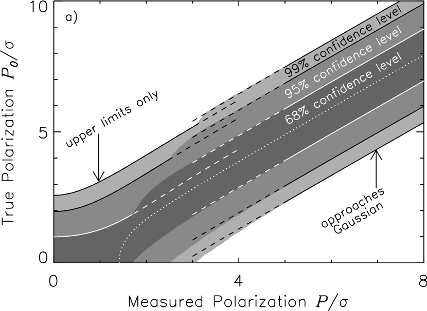
Choosing $\lambda$ such that $(P_{u}-P_{l})$ is minimized implies that $L(P_{l})=L(P_{u})$ (for all $\lambda>0$) but does not generate symmetric confidence regions, especially for low $P/\sigma$. From Figure 3a we see that:

(1) For measured polarization values $P/\sigma<1.7$, 2.4, and 3.0, the lower end of the confidence region is bounded by zero for the 68.0%, 95.0%, and 99.0% confidence levels, respectively. It is not possible to construct a truly bounded symmetric confidence region for these polarizations; it is only possible to construct upper limits ($\lambda=0$).

(2) For polarizations $P/\sigma\gtrsim 4$ the confidence regions approach those given by a normal gaussian distribution centered on the de-biased value $\hat{P}\approx\sqrt{P^{2}-\sigma^{2}}$ ($68\%\rightarrow 1\sigma$, $95\%\rightarrow 2\sigma$, $99.0\%\rightarrow 2.6\sigma$).

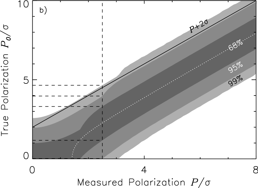
Some authors have placed upper limits of “high confidence” on polarization measurements using the criterion that $P+2\sigma<P_{u}$ (e.g. Dotson et al. 2000). While this criterion matches no single confidence level, it does fall between the 95% and 99% confidence levels even for low $P/\sigma$ (Fig. 3b). For determining upper limits at high confidence this criterion seems a reasonable (and perhaps more feasible) alternative to solving equations (13) and (14).

Figure 3b illustrates the use of our results to find confidence regions. To facilitate comparison of our results with those of SS85, consider a polarization measurement of $P=2\%$, $\sigma=0.8\%$. Upper and lower confidence limits for $P/\sigma=2/0.8=2.5$ are given in Table 1. The differences between the two sets of results increase with increasing confidence level. These differences arise because the integration over data space and subsequent projection onto parameter space performed by SS85 is not equivalent to our integration over parameter space. However, these two methods become congruent as the signal-to-noise increases and the Rice distribution approaches a normal distribution.

Table 1: $P_{0}/\sigma$ confidence regions for $P/\sigma=2.5$

Confidence Level	Simmons & Stewart 1985		This Work
(percent)	Lower	Upper	Lower	Upper
68.0	1.40	3.30	1.20	3.30
95.0	0.28	4.32	0.02	3.97
99.0	0.00	4.96	0.00	4.65

4 Summary

The probability distribution of polarization measurements is asymmetric, resulting in a positive bias and complicating the generation of uncertainties and confidence levels. We generate confidence intervals on the true polarization by integrating the likelihood function over the parameter-space of the true polarization, as opposed to the data-space of the measured polarization. These confidence levels are valid for both high and low signal-to-noise measurements and approach those given by a normal distribution for high signal-to-noise.

References

- Dotson et al. (2000) Dotson, J. L., Davidson, J., Dowell, C. D., Schleuning, D. A., & Hildebrand, R. H. 2000, ApJS, 128, 335
- Eadie et al. (1971) Eadie, W. T., Dryard, D., James, F. E., Roos, M., & Sadoulet, B. 1971, Statistical Methods in Experimental Physics (New York: American Elsevier Publishing Co.)
- Naghizadeh-Khouei & Clarke (1993) Naghizadeh-Khouei, J. & Clarke, D. 1993, A&A, 274, 968
- Rice (1945) Rice, S. O. 1945, Bell Syst. Tech. J., 24, 46
- Simmons & Stewart (1985) Simmons, J. F. L. & Stewart, B. G. 1985, A&A, 142, 100
- Vinokur (1965) Vinokur, M. 1965, Ann. Astrophys., 28, 412
- Wardle & Kronberg (1974) Wardle, J. F. C. & Kronberg, P. P. 1974, ApJ, 194, 249