The Clustering Evolution of Distant Red Galaxies in the GOODS-MUSIC Sample

Abstract

Context.

Aims. We study the clustering properties of Distant Red Galaxies (DRG) to test whether they are the progenitors of local massive galaxies.

Methods. We use the GOODS-MUSIC sample, a catalog of $\sim$3000 Ks-selected galaxies based on VLT and HST observation of the GOODS-South field with extended multi-wavelength coverage (from $0.3$ to $8\mu m$) and accurate estimates of the photometric redshifts to select 179 DRGs with $J-Ks\geq 1.3$ in an area of 135 sq. arcmin.

Results. We first show that the $J-Ks\geq 1.3$ criterion selects a rather heterogeneous sample of galaxies, going from the targeted high-redshift luminous evolved systems, to a significant fraction of lower redshift ($1<z<2$) and less luminous dusty starbursts. These low-redshift DRGs are significantly less clustered than higher-$z$ DRGs. With the aid of extreme and simplified theoretical models of clustering evolution we show that it is unlikely that the two samples are drawn from the same population observed at two different stages of evolution.

Conclusions. High-$z$ DRGs likely represent the progenitors of the more massive and more luminous galaxies in the local Universe and might mark the regions that will later evolve into structures of intermediate mass, like groups or small galaxy clusters. Low-$z$ DRGs, on the other hand, will likely evolve into slightly less massive field galaxies.

1 Introduction

Finding and studying large samples of distant luminous and evolved galaxies is fundamental to provide a deeper insight on the formation of massive galaxies, a process that is commonly perceived as a challenging test for cosmological models of structure formation and evolution. For this reason, in the recent past, the study of early type galaxies at the highest observable redshifts made use of a considerable fraction of large telescope time and occupied a substantial part of the astronomical literature.

The search for passively evolving systems at high redshift began with the so-called Extremely Red Objects (EROs; see also Elston, Rieke & Rieke (1988); Cimatti et al. (2002); McCarthy (2004)) which reproduce the colours of ellipticals at $z\sim 1$. EROs are relatively “new” objects, in the sense that they have been recognized as a specific class only around 1990, due to the availability of Near InfraRed (NIR) detectors only at that epoch. Elston, Rieke & Rieke (1988) found the first two EROs in a survey of 10 sq. arcmin. as resolved galaxies with $K\sim 16.5$ and $R-K\sim 5$. After the optical spectroscopic identifications, the two objects turned out to be an evolved galaxy at $z=0.8$ and a dusty starburst at $z=1.44$, named HR10. It was clear from this survey and successive investigations that the ERO population is heterogeneous in its main properties (star formation, mass, age, extinction, etc.).

At present, there are various techniques to find evolved galaxies at high-$z$. Cimatti et al. (1999) utilised the criterion $R-K\geq 5$(Vega) effective in the redshift interval $0.8\leq z\leq 1.8$ limited to $Ks\leq 20$. Caputi et al. (2004) and Abraham et al. (2004) used a similar selection $I-K\geq 4$(Vega) to select red galaxies with $1\leq z\leq 2$. Pozzetti & Manucci (2000) suggested a two colour criterion ($I-K$ vs $J-K$) to separate ellipticals from dusty starbursts at $1\leq z\leq 2$, which could be extended at higher redshift ($2.0\leq z\leq 2.5$) using redder colours ($J-K$ vs $H-K$). Franx et al. (2003) proposed a simple pure infrared criterion $J-K\geq 2.3$(Vega) for $z\geq 2.0$. In a similar way, Saracco et al. (2004) selected 3 galaxies with $J-Ks\geq 3$(Vega) in the HDFS at $z\geq 2.5$, plausible candidates for high-z massive galaxies, though the statistic is very limited. Recently, Daddi et al. (2004) suggested to isolate early-type galaxies according to the BzK criterion [$(z-K)_{AB}-(B-z)_{AB}\leq-0.2$ and $(z-K)_{AB}\geq 2.5$] efficient at $1.4\leq z\leq 2.5$, and with extension at $2.5\leq z\leq 4.0$ using the RJL colour combination. Yan et al. (2004) proposed a new class of objects, the high-$z$ EROS (called IEROs) with $f_{\nu}(3.6\mu)/f_{\nu}(850nm)\geq 20$ to select red galaxies at $1.5\leq z\leq 3.0$ using MIR data. The physical properties of massive galaxies at high-$z$ were also investigated by Saracco et al. (2005) through spectroscopy of a limited sample of massive, evolved galaxies with relatively bright magnitudes ($K\leq 18.4$) at $1.3\leq z\leq 1.7$ on the MUNICS survey. A different approach has been adopted for the COMBO-17 survey, in which the intrinsic colour (U-V) rest frame is utilised to isolate galaxies belonging to the Red Sequence: Bell et al. (2004) used the relation $(U-V)_{\rm rest}\geq 1.40-0.31\cdot z$, efficient at $0.2\leq z\leq 1.1$ according to simulations with spectral synthesis code. Finally, Giallongo et al. (2005) adopted a slightly different approach: the bi-modality in $(U-V)_{\rm rest}$ is empirically fitted to the observations and could be extended up to $z\sim 3$.

In this paper we focus on the so-called Distant Red Galaxies (DRGs; Franx et al. (2003)). These galaxies are selected through a $J-K>2.3$(Vega) criteria, designed to be sensitive to galaxies with a large 4000 Å  break at $z\geq 2$. Franx et al. (2003) used this technique in the FIRES survey (Labbé et al. (2003)) selecting 14 DRGs in the HDFS, down to faint $Ks$ magnitudes ($Ks\leq 24.5$ in AB mag). By using ultra-deep spectroscopy vanDokkum et al. (2003) provided evidence that the brighter DRGs are indeed galaxies at $z\sim 2$. Even if the evidence for the existence of old and massive galaxies is settled by these observations, however the lack of a statistical significant sample of DRGs hampered the detailed study of many of their properties, in particular their number density, their clustering properties and their physical properties like mass, star formation, age and spectral energy distribution (SED). Recently, Papovich et al. (2005) have derived a sample of 153 DRGs from the GOODS South down to a shallower limit of $Ks=23.2(AB)$, with the aim of studying in detail the specific star formation rate (star formation per unit mass star) of DRGs. They found that the bulk of the star formation in massive galaxies ($M\geq 10^{11}M_{\odot}$) occurs at early cosmic epochs and is largely complete by $z\sim 1.5$.

Analogously to Papovich et al. (2005), we use the extraordinary dataset provided by the GOODS survey to extend these studies. In particular, we will adopt the GOODS-MUSIC sample, a $Ks$-selected sample with an extended wavelength range (from U to $8.0\mu$m band) that we compiled using publicly available data in the Chandra Deep Field South region and described at length in Grazian et al. (2006). With this complete sample of DRGs, we can define in detail their general properties and refine previous investigations by Franx et al. (2003), which used only 14 objects in the FIRES survey, though at a fainter magnitude limit.

The structure of the paper is as follows. In § 2 we describe the data used to analyse DRG properties. In § 3 we select DRGs according to the selection criterion defined by Franx et al. (2003) and provide their number density and the redshift distribution. In § 4 we study the clustering properties of DRGs selected in the GOODS-South field and in § 5 we discuss the link between the DRG population at $z\sim 2$ and the local ellipticals.

All magnitudes, unless otherwise stated, are given in the AB system. A concordance $\Lambda CDM$ cosmological model ($\Omega_{M}=0.3$, $\Omega_{\Lambda}=0.7$ and $H_{0}=70$ km s^-1Mpc^-1) has been adopted throughout the paper.

2 The Data

We use in this paper the data from the Chandra Deep Field South (CDFS; Giacconi et al. (2000)), obtained within the GOODS survey. This is a collaboration between STScI and ESO (Renzini et al. (2003)) that produced an unprecedented dataset of images, covering 135 sq. arcmin. from 0.3 to 8.0$\mu$m down to relatively faint magnitude limits (Giavalisco et al. (2004)). In particular, we used the ACS images (release V1.0, Giavalisco et al. (2004)), the ISAAC database (release V1.0, Vandame et al., in preparation ) and the IRAC dataset (release V1.0 enhanced, Dickinson et al., in preparation ), together with U band photometry from WFI@2.2m ESO-MPI and VIMOS reduced by our group.

Using this public dataset, we have produced a high-quality multicolour catalog of galaxies in the GOODS-South, that we have named GOODS-MUSIC: details about the procedure adopted are discussed in Grazian et al. (2006). We briefly remind here that we have used all the publicly available images from U to 8.0 $\mu$m ($U,B,V,i,z,J,H,Ks,3.6\mu,4.5\mu,5.8\mu,8.0\mu$), in a contiguous area of 135 sq. arcmin., totalling 14847 objects. In particular, to isolate a complete sample of DRGs, we use here the $Ks$-selected sample, that consists of $2931$ galaxies. The GOODS survey has a complex, inhomogeneous exposure map in the $Ks$ band. To properly derive the statistical properties of galaxies in this field, the sample has been divided in 6 sub-areas of different magnitude limits, as described in details in Grazian et al. (2006) and in Tab. 1. This information is used in this work when the DRG statistical properties are studied, such as their number density or clustering properties. The typical magnitude limit for most of the sample is about $Ks=23.5$, and extends down to 23.8 in a limited area.

In Grazian et al. (2006) we included spectroscopic information for 668 galaxies. Recently, Vanzella et al. (2006) have released further spectroscopic redshifts in the GOODS South region. We used this new release to compile a revised sample of 973 galaxies with good spectroscopic identification. Out of this number, 815 are in the $Ks$-selected sample ($\simeq 28\%$ of the total). For the remaining sources, we derived a photometric redshift, as described in Grazian et al. (2006): the redshift accuracy in the range $0<z<6$, as shown in Fig.1, on this enlarged spectroscopic sample is $\sigma_{z}=0.06$, which is the same value previously found in Grazian et al. (2006). If we restrict to the 340 galaxies with red colours ($J-Ks\geq 0.7$), as shown in Fig.2, the redshift accuracy is $\sigma_{z}=0.08$ in the redshift range $0<z<4$.

Figure 1: The spectroscopic vs photometric redshifts for 973 galaxies in the GOODS-MUSIC sample. The accuracy is $\sigma_{z}=0.06$ and $\frac{\sigma_{z}}{1+z}=0.03$ in the redshift range $0<z<6$.

Figure 2: The spectroscopic vs photometric redshifts for 340 red galaxies with $J-Ks\geq 0.7$ in the GOODS-MUSIC sample. The accuracy is $\sigma_{z}=0.08$ and $\frac{\sigma_{z}}{1+z}=0.05$ in the redshift range $0<z<4$. There are only 13 galaxies with $J-Ks\geq 1.3$ and spectroscopic redshifts (red crosses).

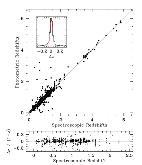
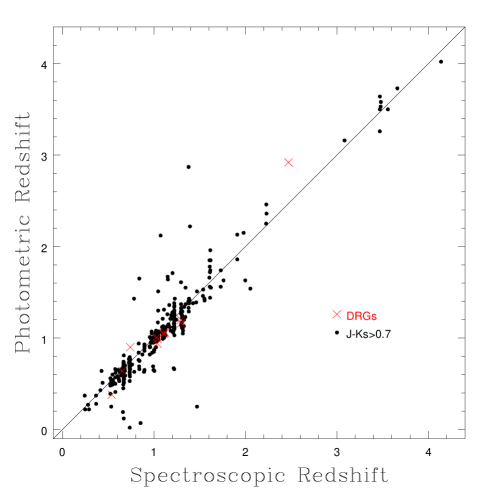
Rest–frame physical quantities (such as luminosities, mass, age, SFR) are derived by using the synthetic library of Bruzual & Charlot (2003) (hereafter BC03), at the spectroscopic redshift, adopting the same technique already described in several previous papers (see Fontana et al. 2004 for more details).

3 Selection of DRGs

3.1 The number density of DRGs

We have selected DRGs according to the criterion defined by Franx et al. (2003), ($J-Ks\geq 1.3$ in AB system, as obtained using the transmission curves for the J and Ks filters of ISAAC), which is efficient at $z\geq 2$. Fig. 3 shows the effect of this selection criterion of DRGs applied to the objects of GOODS-MUSIC sample.

Figure 3: Selection of $J-Ks\geq 1.3$ objects in the GOODS-South Field. Upper limits in the $J$ band are shown as vertical arrows. The horizontal line shows the selection criteria for DRGs in the GOODS-South area, while dashed line indicates the completeness on the DRG selection due to the depth of the J band (26.8 AB at $S/N=1$).

In the GOODS-South region we find 179 galaxies having $J-Ks\geq 1.3$. For the reasons described above, the completeness limit of the survey is not homogeneous, with a typical value of $Ks=23.5$. We use this sample of DRGs to study in particular their number density and their spatial distribution (clustering).

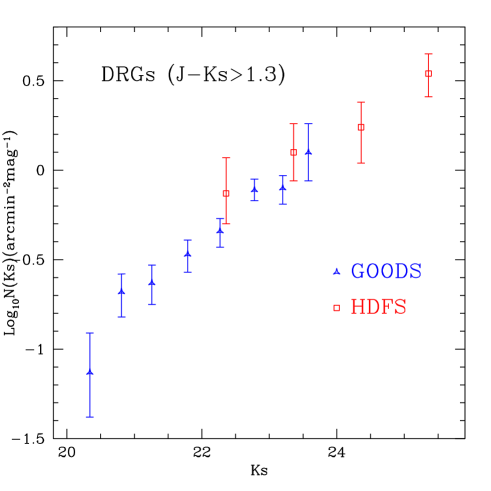
The number density of DRGs in the GOODS South field is derived through the classical $\log N-\log S$ distribution, or the number of objects per sq. arcmin. and per magnitude bin in the $Ks$ band. This last quantity is obtained by following the recipe of Avni & Bahcall (1980):

$$n(Ks)=\frac{1}{\Delta Ks}\sum_{i=1}^{N_{\rm obj}}\left[\sum_{j=1}^{N_{\rm field}}Area_{j}^{\rm max}\right]^{-1}\ ,$$ (1)

where the sum is on the $N_{\rm field}$ surveys (here, the 6 areas with different magnitude limits described in Grazian et al. (2006) and in Tab.1) and on the $N_{\rm obj}$ objects; $Area_{j}^{\rm max}$ represents the accessible area of the $j$-th survey (this is equivalent to the maximum accessible volume when the luminosity function is derived). The DRG counts have been computed in bins of $\Delta Ks=0.5$ magnitude.

Fig. 4 shows the surface density of DRGs in the GOODS South field and compares it with the results derived in the HDFS by the FIRES survey (Labbé et al. (2003)). Even if the area of HDFS is smaller with respect to the GOODS Survey, the DRG number densities in these two independent fields are comparable (see also Table 1). Notice, however, that different values for the number density of DRGs has been derived by using the data of the HDFN (Lanzetta et al. (1998); Fontana et al. (2000); Dickinson (1998)), in which one DRG is found at $Ks\leq 23.0$, and a limited number at $23\leq Ks\leq 24$ with upper limit in the $J$ band. The sample variance between HDFN and HDFS is due to the limited area investigated and stresses the necessity of deriving a firm measurement for the number density of DRGs in a large and deep survey such as the GOODS-CDFS field.

Figure 4: The surface density of selected DRGs in the GOODS-South Field (triangles), compared with the estimate obtained in the HDFS (squares, Labbé et al. (2003)).

Table 1: Number density $\Sigma$ of DRGs in the $Ks$ band for GOODS-South and HDFS fields

$bin$	$N$	$\log(\Sigma)$	$\bar{z}$	$\bar{Ks}$	AREA
		mean $+1\sigma$ $-1\sigma$			$arcmin^{2}$
20.25	6	-1.13 -0.91 -1.38	1.05	20.34	135.372
20.75	14	-0.68 -0.58 -0.82	1.25	20.81	135.372
21.25	16	-0.63 -0.53 -0.75	1.42	21.26	135.372
21.75	22	-0.47 -0.39 -0.57	1.96	21.79	129.692
22.25	29	-0.34 -0.27 -0.43	2.04	22.27	128.273
22.75	50	-0.11 -0.05 -0.17	2.45	22.78	127.935
23.25	32	-0.10 -0.03 -0.19	2.80	23.20	81.272
23.75	10	0.10 0.26 -0.06	2.75	23.58	12.585
22.50	4	-0.13 0.07 -0.30	2.75	22.36	4.500
23.50	7	0.10 0.26 -0.06	2.75	23.36	4.500
24.50	8	0.24 0.38 0.04	2.75	24.36	4.500
25.50	18	0.54 0.65 0.41	2.75	25.36	4.500

• a) the number density $\Sigma$ is in units of $arcmin^{-2}mag^{-1}$

• b) $bin$ represents the central bin magnitude in $Ks$

• c) $\bar{z}$ and $\bar{Ks}$ are the mean values of redshift and observed $Ks$ magnitude for each magnitude bin

• d) the number density in the second half of the table derives from the FIRES survey in the HDFS (Labbé et al. (2003))

3.2 Redshift distribution of DRGs

Figure 5: Upper panel: the distribution of spectroscopic (only 13 objects; short-dashed line) and photometric (solid line) redshifts of selected DRGs in the GOODS-South Field. The dotted curve is the redshift distribution obtained for the DRGs using the probability function for the redshift for each object derived by the photometric redshift code. It is in agreement with the distribution using the best estimate for the photometric redshift code. The long-dashed line represents the redshift distribution for the HDFS (Labbé et al. (2003)), peaked at $z\sim 3$. It is markedly different from the redshift distribution of the GOODS field, since DRGs in the HDFS have fainter $Ks$ magnitudes. The redshift distribution of HDFS is comparable to the redshift distribution of DRGs in the GOODS field at $Ks>23$ magnitude, as shown in the lower panel. Lower panel: the photometric redshift distribution for bright ($Ks<22$; long-dashed line) and faint ($Ks>22$; solid line) DRGs. Deep pencil beam surveys (HDFs) preferentially select objects at $z\sim 2$, while large area surveys are biased towards lower-redshift ($z\leq 2$) and bright ($Ks<22$) DRGs (short-dashed line).

Figure 6: The $J-Ks$ colour of objects in the GOODS-South field as a function of their (spectroscopic or photometric) redshift. Upper limits in the $J$ band are displayed as vertical arrows. The long-dashed horizontal line shows the selection criteria adopted for DRGs in this paper. The two blue solid lines show the $J-Ks$ colour for passively evolving galaxies formed at $z=20$ and with an e-folding star formation rate with timescale $\tau=0.1$ and $\tau=1$ Gyr (upper and lower curves, respectively). The red short-dashed lines show the same colour for a star-forming galaxy with $E(B-V)=1.1$ and $E(B-V)=0.5$ (upper and lower curves, respectively).

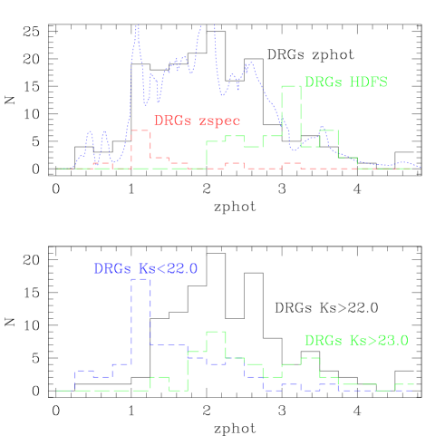
The large number of DRGs in the GOODS field makes it possible to test the selection criterion and to define the window function in redshift for DRGs. Fig. 5 shows the distribution of the photometric redshifts of DRGs: the spectroscopic sample of DRGs is very limited both in redshifts and $Ks$ magnitudes (only 13 galaxies with $19.7\leq Ks\leq 22.9$ and $0.65\leq z\leq 3.04$). The redshift distribution of GOODS DRGs is slightly different from that drawn for HDFS by Franx et al. (2003) and Daddi et al. (2003), which covers the interval $2\leq z\leq 4$ with a prominent peak at $z\sim 3$, and in reasonable agreement with the similar analysis of Papovich et al 2005. In our GOODS-MUSIC sample there are DRGs at lower redshifts ($1\leq z\leq 2$) with bright apparent $Ks$ magnitudes ($Ks\leq 22$), which are in practice absent in small and deep pencil beam surveys, like the HDFS. The redshift distribution clearly shows that there is a considerable fraction (77 out of 179, i.e. 43$\%$) of objects at low redshifts ($z\leq 1.9$) which satisfy the $J-Ks$ selection. With a typical colour $J-Ks\sim 1.5$, they cannot be the result of photometric errors, since this should be negligible for relatively bright objects: in fact at $Ks\sim 21.5$ the typical error in magnitude is $\sigma=0.03$. The SEDs of these low-redshift DRGs are dominated by power-law spectra with a tilt at $\lambda\sim 6\mu m$, which are mostly fitted by relatively young galaxies (${\rm age}/\tau\leq 1$) and a substantial amount of extinction ($E_{B-V}\sim 0.5-1.0$, see Fig. 8 of Papovich et al. (2005)).

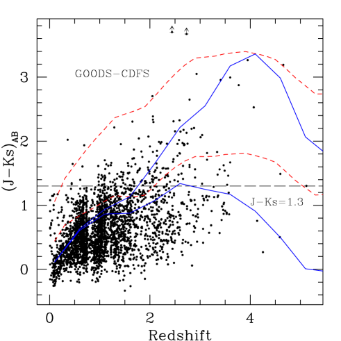
Fig. 6 may help in understanding this result, which is due to the complex selection effects that are effective in this colour criterion. In Fig. 6 we compare the observed $J-Ks$ colour as a function of redshift with the expected $J-Ks$ of a few, selected templates computed with the BC03 models. Two of these models are computed adopting exponentially declining star-formation histories, both started at very high redshift ($z_{\rm form}=20$), with solar metallicity. The values adopted for the e-folding timescale ($\tau=0.1$ and $\tau=1$ Gyr) both produce the same colour at low redshift and show that the $J-Ks>1.3$ threshold is effective in selecting galaxies at $z>2$ that formed their stars in a short starburst $\tau\leq 1$Gyr. At the same time, large $J-Ks$ colours may be obtained by star-forming, dusty models down to lower redshift $z\simeq 1$.

This highlights why the DRG population is not a unique class of $z>2$ objects, but it is contaminated by dusty starbursts with $z\sim 1.5$, whose strong dust absorption is responsible for their red infrared colours. The low-redshift DRG sub-sample is at the limit of the $J-Ks$ selection, and can be explained by dust reddening of $z\sim 1.5$ star-forming galaxies, as shown in Fig. 6. If a more drastic cut $J-Ks$ colour would be applied (e.g. $J-Ks\geq 1.8$), this would ensure a much more efficient selection of galaxies with $z\geq 2$, but the sample would be strongly reduced, from 179 to 51 galaxies only.

Figure 7: The distribution of the ratio between the age of DRGs and the characteristic timescale $\tau$ of the exponentially declining SFR, according to the BC03 spectral synthesis model. The solid histogram refers to the distribution of low-$z$ DRGs, dominated by relatively young objects (age/$\tau\leq 3$) which are typically dusty starbursts, while the dashed histogram shows the ratio for $2\leq z\leq 4$ DRGs, where a considerable fraction (30%) of old and passively evolving galaxies arise.

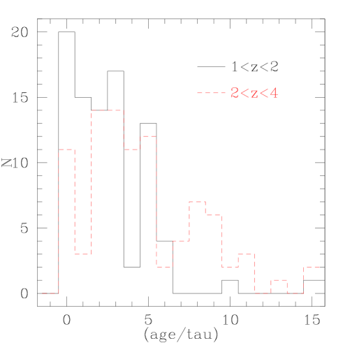
The difference between low-$z$ and high-$z$ DRG has been extensively discussed in a recent paper by Papovich et al. (2005). They argue that lower-$z$ DRG are dominated by dusty starbursts, while the higher-$z$ objects are made of a more complex stellar population, likely a mixture of star-forming, heavily extincted and older, passively evolving stellar components, with a minority of galaxies that are likely genuinely passively evolving. In our preliminary, simplified analysis (the most important difference with respect to Papovich et al. (2005) is that we do not use models with two-component stellar populations and we do not include the $24\mu$ data in the analysis) we also have evidence of the same distinction. This is shown in Fig.7, where we report the distribution of the ratio between the fitted age and the fitted star-formation e-folding timescale $\tau$ (such a ratio is in practice the inverse of the Scalo parameter). As it is shown, all low-$z$ DRG are dominated by actively star-forming, relatively young objects, while higher-$z$ DRGs have a broader distribution of age$/\tau$, including several objects (30% of the high-$z$ DRG sample) that are fitted by passively evolving models.

The average luminosities in the rest–frame I band (Vega system) that we infer from the spectral fitting of our sample are $<M_{I}>=-22.3$ and $<M_{I}>=-23.2$ at $<z>=1.5$ and $<z>=2.7$, respectively, and the average stellar masses are $<M_{*}>=8.15\cdot 10^{10}M_{\odot}$ and $<M_{*}>=9.90\cdot 10^{10}M_{\odot}$ (10.76 and 10.88 if we compute $<\log(M)>$), respectively.

It is tempting to speculate on the possible spectral evolution of these objects. A lower limit to their local luminosity can be obtained by assuming that they enter into a passive evolution phase soon after we observe them. In this case, assuming a truncated star-formation history with solar metallicity, the BC03 code predicts in the rest-frame I band a fading from $<z>=1.5$ and $<z>=2.7$ to $z\simeq 0$ of 2.2 and 2.45 magnitudes, respectively. However, we have to take into account that DRG are typically dusty objects, such that we should probably normalise this fading to their unobscured luminosity. Assuming that the typical reddening of DRG is $E(B-V)\simeq 0.75\pm 0.25$ with a Calzetti extinction curve, and that they evolve to present-day objects with little dust extinction, we find that the typical change in rest-frame magnitude $\Delta M_{I}=M_{I}(z)-M_{I}(z=0)$ is $0.26\pm 0.65$ at $<z>=1.5$ and $-0.49\pm 0.65$ at $<z>=2.7$. Given the average rest frame luminosities described above, this would imply that the descendents of DRG in this simple model have rest frame luminosities of about $M_{I}(z=0)=-22.56$ and $-22.71$. The typical $M^{*}$ magnitude in the I band for local galaxies in the SDSS is $M_{i}=-22.48$ (Blanton et al. (2001)), which increases to $-23.2$ if one considers only the reddest galaxies ($g-r\geq 0.74$). Considering that it is obviously implausible that all DRGs are observed at the end of their star–forming phase, and that therefore they will end up in more luminous and massive objects than predicted by this exercise, one can conclude that both the low-$z$ and high-$z$ DRGs are consistent with being the progenitors of local massive galaxies. The analysis of clustering will help to clarify this conclusion.

4 Spatial distribution of DRGs: the clustering properties

It is already known that DRGs are not uniformly distributed on the sky, but they are clustered on scales of several Mpc. The analysis of the HDFS shows that the DRGs are in prevalence concentrated in one quadrant of the WFPC, while in the HDFN there is only one DRG, suggesting that this population could be strongly clustered and affected by cosmic variance (Vanzella et al. (2001); Franx et al. (2003); Daddi et al. (2003)), such that the small area covered by surveys like HDFN or FIRES prevents to derive a robust measurement of their clustering properties and their redshift evolution.

We therefore present in the following a detailed analysis of the clustering properties of our GOODS-MUSIC DRG sample. Thanks to the available statistics, we will consider both the overall sample, similarly to what already done in previous works, but we will also divide the sample into two different sub-groups: the first one, containing objects with $1<z<2$, where the dusty starburst population is expected to be the dominant component; the second one, containing objects with $2<z<4$, where also relatively evolved galaxies are represented in the sample.

Figure 8: The angular distribution of selected DRGs in the GOODS-South Field. The symbols are coded according to the redshift: DRGs at $z\geq 2$ and at $z\leq 2$ are shown by red triangles and blue circles, respectively; black dots refer to normal galaxies at all redshifts. For comparison, the size of the HDF is also shown. The DRGs are clustered and not uniformly distributed over areas larger than the HDFs: this shows that the cosmic variance for DRGs is dramatic at small scales.

4.1 Angular Two Point Correlation Function

We have used the Landy-Szalay estimator (Landy & Szalay (1993)) to obtain the two-point correlation function (TPCF) in the angular coordinates ($\alpha$,$\delta$) for DRGs in the GOODS Field:

$$w(\theta)=\frac{GG(\theta)-2GR(\theta)+RR(\theta)}{RR(\theta)}\ ,$$ (2)

where $GG(\theta)$ is the number of observed galaxy pairs at distance between $\theta$ and $\theta+d\theta$, $GR(\theta)$ is the number of observed-random pairs and $RR(\theta)$ is the random-random pairs. We compute $GR$ and $RR$ as mean values of 1,000 simulated random catalogs. The random sample of galaxies is obtained by randomly generating the coordinates ($\alpha$,$\delta$) in the GOODS-CDFS field. Each random galaxy is then retained or rejected according to the magnitude limit at the selected position. This ensures to correctly reproduce the selection function of observed DRGs, even in presence of a complicated exposure map, like the GOODS survey one (Grazian et al. (2006)). Finally we correct the observed $w(\theta)$ taking into account the bias arising from the finite boundary of the sample (see the details in Appendix A).

Errors on the angular correlation function, $\sigma_{w}$, are determined by Poisson statistics, through the relation

$$\sigma_{w}=\sqrt{\frac{1+w(\theta)}{GG(\theta)}}\ .$$ (3)

We fit the angular correlation function (computed in annuli of increasing $\theta$) by a power-law relation, $w(\theta)=(\theta/\theta_{0})^{-\delta}$, fixing $\delta=0.8$. Following Croft et al. (1997) (see also Croom et al. (2002); Grazian et al. (2004)) the fit is carried out by using a Maximum Likelihood Estimator (MLE) based on Poisson statistics and unbinned data. A detailed description of the MLE can be found in Appendix A.

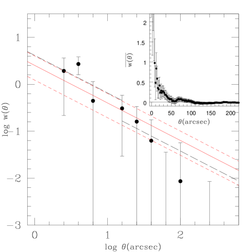
The results for the DRG TPCF are presented in Fig. 9 (large quadrant), together with the MLE fit with the corresponding 1$\sigma$ confidence intervals. Considering the interval $1\leq\theta\leq 100$ arcsec, we find a clustering scale of $\theta_{0}=3.19^{+2.48}_{-1.90}$ arcsec. The mean redshift and absolute magnitude for the clustered galaxies are $z_{\xi}=2.1$ and $M_{I}=-22.8$, respectively. The small quadrant of Fig. 9 shows the TPCF integrated in circles of increasing apertures $\theta$. We do not use this quantity to fit the best value for $\theta_{0}$, since errors are correlated in different bins of angular separation. However, we can obtain from its value an indication of the clustering strength: at $\theta=12$ arcsec we observe 23 pairs, while simulations of random distributions predict 12 pairs only, which is a detection at about 3$\sigma$; at $\theta=6$ arcsec we derive an excess of 7 pairs over 3 random, which represents a 4$\sigma$ detection.

By looking at the integrated angular TPCF shown in the small quadrant of Fig. 9, we notice that it is still significantly non null even at large scales ($\theta\approx 50-60$ arcsecs), which are comparable to the angular size of the HDFs. This result confirms that the difference in the DRG number density found in previous surveys is due to both the cosmic variance and their strong clustering, whose effects can become dramatic when considering deep pencil beam surveys, which are conducted over small areas, like the HDFs or the Hubble Ultra Deep Field (HUDF, Beckwith et al. (2003)).

To have a look at the redshift evolution of the DRG clustering properties, we compute the correlation scale of the low- and high-redshift samples, separately, and find a clear evidence of a strong evolution: we indeed estimate a correlation scale of $\theta_{0}=3.69_{-3.35}^{+5.03}$ arcsec ($z_{\xi}=1.5$ and $M_{I}=-22.30$) for the low-redshift sample (76 galaxies), and $\theta_{0}=13.68_{-6.29}^{+7.84}$ arcsec ($z_{\xi}=2.7$ $M_{I}=-23.20$) for the high-redshift one (88 galaxies).

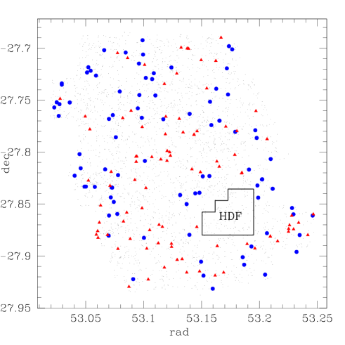
We note that it is well known that at small scales ($\theta\leq 10$ arcsec) the TPCF is dominated by substructures, produced by the existence of multiple galaxies inside massive halos (see, e.g. Lee et al. (2005)). This effect is also evident in Fig. 8, where the presence of close-by galaxy pairs or triplets is clearly visible. To measure the clustering properties of dark matter halos (DMHs) hosting DRGs, it is necessary to avoid using only the smallest scales, where the halo occupation distribution (HOD) is plausibly larger than unity. Using the total DRG sample, we obtain a correlation length of $\theta_{0}=5.89^{+3.74}_{-3.10}$ arcsec for $\theta\leq 10$ arcsec, while in the interval $10\leq\theta\leq 100$ the TPCF is significantly weaker, with a MLE fit of $\theta_{0}=1.67^{+2.17}_{-1.50}$ arcsec (see the long dashed lines in Fig. 9). It is important to remark, however, that the redshift evolution is clearly detected at both scales, although the uncertainties become obviously much larger. At the scale of $\theta\leq 10$, indeed, the correlation length is $\theta_{0}=3.84^{+7.15}_{-3.46}$ arcsec at $1<z<2$ and $\theta_{0}=15.52^{+9.28}_{-7.60}$ arcsec at $2<z<4$. At $10\leq\theta\leq 100$, the correlation length is $\theta_{0}=2.89^{+3.90}_{-2.65}$ arcsec at $1<z<2$ and $\theta_{0}=8.48^{+13.20}_{-6.72}$ arcsec at $2<z<4$. Notice that in our following discussion we will use the clustering length obtained by the fit over the global range $1\leq\theta\leq 100$ arcsec, since it is a robust compromise against boundary effects at the largest scales and against HOD effect at the smallest scales.

Figure 9: Large panel: the differential angular TPCF (in a logarithmic scale) for the DRGs in the GOODS field (filled circles with 1$\sigma$ error bars). We also plot the MLE best fit power-law relation (solid line) with its 1$\sigma$ confidence interval (short-dashed line), as computed in the interval $1\leq\theta\leq 100$ arcsec: the corresponding correlation scale of DRGs is $\theta_{0}=3.19$ arcsec. The two dotted lines refer to the MLE best fits on limited intervals: $\theta\leq 10$ arcsec and $\theta\geq 10$ arcsec. Note that at small scales the TPCF is enhanced by the presence of multiple galaxies in the same DMH, while at large scales the boundary effect may become critical. Small quadrant: the angular TPCF integrated over circles of increasing radii (filled circles with 1$\sigma$ error bars).

4.2 Spatial clustering

To convert the angular correlation length to physical units we can invert the angular TPCF through the Limber equation (Limber (1953)), adopting the DRG redshift distribution presented in Fig. 5. Leaving the detailed calculations to Appendix A, we have:

$$w(\theta)=\frac{r_{0}^{\gamma}\theta^{1-\gamma}I(\gamma)\int_{0}^{\infty}(\frac{dN}{dz})^{2}r(z)^{1-\gamma}(\frac{dz}{dr})dz}{N^{2}_{\rm obj}}\ ,$$ (4)

where $I(\gamma)=3.67909$ when $\gamma=1.8$ is assumed.

Using the value for $\theta_{0}=3.19^{+2.48}_{-1.90}$ derived through the MLE fit to the angular TPCF, for the complete DRG sample, we obtain a correlation length of $r_{0}=9.78^{+2.85}_{-3.24}h^{-1}$ Mpc. Using the same Limber equation, the corresponding comoving correlation lengths are $r_{0}=7.41^{+3.45}_{-4.84}h^{-1}$ Mpc and $r_{0}=13.36^{+2.99}_{-3.20}h^{-1}$ Mpc, for the sub-samples at $1<z<2$ and $2<z<4$, respectively.

We note that the TPCF for the higher-redshift sub-sample is different with respect to the value obtained by Daddi et al. (2003) for DRGs in the HDFS, although still marginally consistent, because of the relatively large error budget. We have to notice, however, that for their analysis they applied a colour selection criterion which is bluer ($J-Ks\geq 0.7$) than the one adopted here ($J-Ks\geq 1.3$). We tested that, by selecting in the GOODS region DRGs at $2\leq z\leq 4$ with their same colour cut, we obtain a sample of 232 galaxies, with a typical redshift of $z_{\xi}=2.9$, having a correlation length of $r_{0}=8.8\pm 1.7h^{-1}$ Mpc, which is comparable to the value provided by Daddi et al. (2003) ($8.3\pm 1.2h^{-1}$ Mpc). A redder cut ($J-Ks\geq 1.3$) applied for DRGs in the HDFS actually results in a larger correlation length of $r_{0}=14.5^{+3.1}_{-3.7}h^{-1}$ Mpc (Daddi et al. (2003)), which is consistent with our estimate.

As a further comment, we also notice that the error associated to our estimate for $r_{0}$ in our whole sample ($\sim 3h^{-1}$ Mpc) is slightly higher than the value quoted by Daddi et al. (2003) for the DRGs in the HDFS, even if the samples have a different number of objects (197 DRGs in GOODS against 49 in the HDFS). This is due to the fact that we include in the error budget the effects of cosmic variance, which is the dominant effect in this kind of study and it is not included in the error bars quoted for DRGs in HDFS.

It is interesting to compare these results with other estimates of clustering strength, for other related classes of objects. In order to avoid the dependence of the scale length $r_{0}$ on the power-law fit $\gamma$, it can be useful to present the results in a non-parametric form. This can be done by using the quantity $\bar{\xi}$, defined as the correlation function $\xi(r)=(r/r_{0})^{-\gamma}$ integrated over a sphere of a given radius $r_{\rm max}$:

$$\bar{\xi}(r_{\rm max})=\frac{3}{r_{\rm max}^{3}}\int_{0}^{r_{\rm max}}\xi(x)x^{2}{\rm d}x\ .$$ (5)

In general, the larger the scale on which the clustering is measured, the easier the comparison with the linear theory of the structure evolution. Since in the following we want to compare our results with those obtained for different values for $\gamma$, we prefer to quote clustering amplitudes within $20h^{-1}$ Mpc, a scale for which linearity is expected to better than a few per cent. Choosing a large radius also reduces the effects of small scale peculiar velocities and redshift measurement errors, which can be a function of redshift.

Fig. 10 compares the values for $\bar{\xi}(20h^{-1})$ that we obtained for DRGs in the GOODS field (summarised in Table 2) to the corresponding estimates for other classes of objects, both at low and high redshift. It is immediately clear that the high-redshift ($z>2$) sample of DRG is drawn from a remarkably highly clustered population, most likely more clustered than the $z<2$ DRG population.

At $z=0$, the only galaxies having correlation lengths as large as 10-11 $h^{-1}$ Mpc (corresponding to $\bar{\xi}(20h^{-1})\sim 1$) are morphologically-selected giant ellipticals or radio-galaxies. Guzzo et al. (1997) estimate $r_{0}=8.35\pm 0.76h^{-1}$ Mpc for early-type galaxies with $M_{B}\leq-19.5+5log(h)$ in the Pisces-Perseus super-cluster survey, while Adami & Mazure (2002) derive a significantly smaller value ($r_{0}=7h^{-1}$ Mpc with $\gamma=-1.79$) from the SSRS2 redshift survey. The discrepancy between these two measurements is probably originated by the presence in the first survey of the super-cluster, which enhances the correlation function. Overzier et al. (2003) and Rottgering et al. (2003) find that local radio-galaxies have large clustering lengths (see also Peakcock & Nicholson (1991)) and that the high degree of correlation between hosting ellipticals and luminous radio-sources suggests an interesting possible comparison for distant samples.

For small groups of galaxies in the local Universe, the typical value for $\bar{\xi}$ has been measured by Girardi et al. (2000); Zandivarez et al. (2003); Padilla et al. (2004), and again shown in Fig.10. Collins et al. (2001) report the results of the spatial two-point correlation function for the galaxy cluster survey ROSAT-ESO Flux-Limited X-ray (REFLEX), finding $\bar{\xi}(20h^{-1})=2.29\pm 0.50$ for rich clusters at $z\leq 0.3$.

More ordinary elliptical galaxies show a range of clustering strength, that is strongly dependent on the absolute magnitude. We reproduce in Fig. 10 the range corresponding to local elliptical galaxies ranging from $M_{B}=-17$ to $M_{B}=-21$, taken from Norberg et al. (2002) and Zehavi et al. (2002).

At high redshifts, we also display the values observed for EROs (Daddi et al. (2000)) and for bluer DRG (Daddi et al. (2003)).

This compilation of clustering strength for a wide range of objects shows that DRG are among the mostly clustered objects at galactic scales, and suggests that they might be related to the progenitors of similarly clustered objects at lower redshifts, as EROs or local massive ellipticals. Unfortunately, a firm conclusion in this context is not straightforward, since we do not know the evolution of the bias parameter for this class of high-redshift objects. This point will be better discussed in the final section.

Figure 10: The integrated clustering strength $\bar{\xi}(20h^{-1}Mpc)$ as a function of redshifts for different objects: DRGs, EROs, powerful radio-galaxies, ellipticals and galaxy groups/clusters. Filled squares show the results for low- and high-$z$ DRGs in the GOODS region, while void square represents the whole DRG sample. The solid lines show the predicted evolution of the clustering according to the object-conserving model, tuned to the DRGs at low- and high-$z$, while the dashed lines reproduce the clustering evolution according to the merging model. The plot suggests that high-redshift DRGs can be the progenitors of local ellipticals, but may evolve into more massive objects, like EROs at $z\sim 1$ and groups/clusters of galaxies in the local universe. The horizontal error bars show the redshift intervals for the DRGs in this work. Filled triangles show the values of the correlation strength for DRGs with $J-Ks\geq 0.7(AB)$ as estimated in the HDFS (Daddi et al. (2003)) at $z=3.1$ and in the GOODS region at $z=2.9$ (this work).

Table 2: Clustering properties of DRGs

$Type$	$r_{0}$	$\gamma$	$\bar{\xi}(20h^{-1})$	$z$	$M_{I}$
	($h^{-1}$ Mpc)
DRGs	$9.78^{+2.85}_{-3.24}$	1.8	$0.690^{+0.403}_{-0.356}$	2.1	-22.8
low-$z$ DRGs	$7.41^{+3.45}_{-4.84}$	1.8	$0.419^{+0.414}_{-0.357}$	1.5	-22.3
high-$z$ DRGs	$13.4^{+2.99}_{-3.20}$	1.8	$1.209^{+0.530}_{-0.470}$	2.7	-23.2
$J-Ks\geq 0.7$	$8.77^{+1.62}_{-1.70}$	1.8	$0.657^{+0.112}_{-0.272}$	2.9	-23.0

5 Summary and Discussion

In this paper we have presented an analysis of Distant Red Galaxies (DRG) selected in the GOODS-South region. In particular, we have used the GOODS-MUSIC sample, that has been compiled from a unique dataset that comprises accurate multi-wavelength coverage (14 bands from $0.3$ to $8\mu m$) of $\sim$3000 galaxies in $Ks$ complete sample, with accurate estimates of the photometric redshifts for all galaxies in the field. From the GOODS-MUSIC sample, we have selected 179 DRGs according to the criterion proposed by Franx et al. (2003), $J-Ks\geq 1.3$ at a typical magnitude limit of $Ks=23.5(AB)$ and down to $Ks=23.8$ in a limited area. The wide and deep covered area (135 sq. arcmin), together with the extended SED information and the precision in photometric redshifts ($\sigma_{z}=0.06$), allows to study the statistical properties of DRGs, like the redshift distribution, number density and clustering properties at an unprecedented level.

The derived number density is consistent with that found by Labbé et al. (2003), with approximatively 1 DRG per sq. arcmin. at $Ks=23.5$. The redshift distribution shows a smoothed peak around $z\sim 2$, with extended tails both to $z=1$ and $z=4$. Bright DRGs ($Ks\leq 22$) tend to dominate the $z\sim 1$ region, while apparently faint DRGs ($Ks>22$) are distributed widely around $z\sim 2.0-3.5$. The two populations also have different intrinsic properties: low-redshift DRG are slightly less luminous than their higher-$z$ counterparts ($<M_{I}>=-22.3$ and $<M_{I}>=-23.2$, respectively), and possibly slightly less massive ($<M_{star}>=8.15\cdot 10^{10}M_{\odot}$ and $<M_{star}>=9.90\cdot 10^{10}M_{\odot}$, respectively).

In particular, we investigated on the spatial distribution of DRGs through the Two-Point Correlation Function (TPCF) analysis. We find that DRGs from the overall sample are significantly clustered (4$\sigma$ detection), with a typical correlation length of $\theta_{0}=3.19^{+2.48}_{-1.90}$ arcsec, corresponding, through the Limber equation and the observed redshift distribution, to $r_{0}=9.78^{+2.85}_{-3.24}h^{-1}$ Mpc. We also find that the clustering strength of DRGs increases with the $J-Ks$ colour cut used for selection.

Using the relatively large sample of DRG provided by the GOODS-MUSIC sample, we divided the DRG sample in two sub-groups in redshift, one with $1\leq z\leq 2$ and the other with $2\leq z\leq 4$. The clustering of low-$z$ DRGs is significantly lower than that of the high-$z$ DRGs, with $r_{0}=7.41^{+3.45}_{-4.84}h^{-1}$ Mpc and $13.4^{+2.99}_{-3.20}h^{-1}$ Mpc, respectively. It is useful to stress here that this behaviour is not due to a physical evolution of the DRG population. It is the result of a selection criterion which provides an heterogeneous group of dusty starburst and massive/evolved galaxies with different redshift distribution.

Unfortunately, a direct comparison of the clustering properties of DRGs with those of other objects can be misleading, since it is not known a priori the connection between these classes. However, it is possible to constrain the clustering evolution of the descendents of the DRG population using two extreme, simplified models, as proposed by Matarrese et al. (1997) and Moscardini et al. (1998) for the merging of galaxies in a $\Lambda$CDM hierarchical clustering scenario. In one case, that was named object-conserving model, we assume that the observed DRGs do not undergo any subsequent phase of merging with other objects, included those of lower mass. This model, which is conceptually close to a sort of “passive evolution” scenario, assumes that the galaxies form at some characteristic redshift by some non-linear process which induces a bias parameter at that epoch, and that their subsequent motion is purely caused by gravity, following the continuity equation. An obvious consequence of this model is that the bias factor will not be constant for all time, but will tend to unity as time goes on because the galaxies will be dragged around by the surrounding density fluctuations, populated by less clustered objects. This scenario, which corresponds to have an extremely long merging or disruption time, provides an upper limit to the evolution of the clustering properties of DRG descendents, and is shown as thick solid lines in Fig.10, after normalisations to the DRG values obtained in this paper. On the other side, we use a merging model, where the - even more extreme - assumption is that galaxies continue the merging process down the lowest redshifts, with the same (high) merger rate of their parent halos. This clearly extreme model provides a lower limit of the evolution of the clustering properties of DRG descendents, and is shown as dashed lines in Fig.10. These theoretical predictions have been obtained adopting the standard $\Lambda CDM$ power spectrum, normalised to reproduce the local cluster abundance ($\sigma_{8}=0.9$).

Although the error budget on the estimate of $\bar{\xi}(20h^{-1})$ on the two DRG samples is still relatively large, we can use these two limiting theoretical predictions to attempt a physical interpretation of our results.

First, the observed value of $\bar{\xi}(20h^{-1})$ for the low-$z$ DRGs is outside the range predicted for the evolution of the higher $z$ sample: this suggests that is unlikely that the two samples are drawn from the same population, observed at two different stages of evolution.

If we look at the low redshift range predicted for the DRG evolution, it is suggested that high-redshift DRGs (i.e. those typically selected at $Ks>22$, see Fig.5) likely represent the progenitors of the more massive galaxies in the local Universe, i.e. the more luminous ellipticals, and might mark the regions that will later evolve into structures of intermediate mass, like groups or small clusters.

On the other hand, low-redshift DRGs (i.e. those typically selected at $Ks<22$), will likely evolve into slightly less massive field galaxies, approximately around the characteristic luminosity $L^{*}$ of local ellipticals.

Our observations provide further evidence for the so called “downsizing” scenario that has emerged in many different aspects of high redshift galaxies, providing evidences that more massive galaxies have formed preferentially at higher redshifts than less massive ones. Here we find the same trend, since high redshift DRGs are more clustered, more luminous, and most likely to evolve into more massive galaxies than their lower-$z$ counterparts.

Appendix A The Two-Point Correlation Function and the Limber Equation

The calculation of the TPCF over small regions of the sky is affected by boundary effects. This bias, known as the integral constraint, is produced by the fact that the angular TPCF is computed over a limited area $\Omega$: the consequence is a reduction of the amplitude of the correlation function by

$$w_{\Omega}=\frac{1}{\Omega^{2}}\int\int w(\theta)d\Omega_{1}d\Omega_{2}\ .$$ (6)

Following Roche et al. (2002) we estimated $w_{\Omega}$ numerically as

$$w_{\Omega}=kA_{w}=\frac{\sum{RR(\theta)A_{w}\theta^{-\delta}}}{\sum{RR(\theta)}}\ ,$$ (7)

where we assumed for $w(\theta)$ a power-law relation: $w(\theta)=A_{w}\theta^{-\delta}$. Fixing $\delta=0.8$ we obtain $w_{\Omega}=10.692A_{w}$ and the corrected expression for the angular TPCF becomes

$$w(\theta)=w^{\rm obs}(\theta)+w_{\Omega}\ .$$ (8)

The fit of the differential angular TCPF (corrected for boundary effects and computed in annuli of increasing $\theta$) is carried out by using a Maximum Likelihood Estimator (MLE), described in Croft et al. (1997). This method is based on Poisson statistics and unbinned data. Unlike the usual $\chi^{2}$ minimisation, MLE avoids the uncertainties related to the bin size, the position of the bin centre and the bin scale (linear or logarithmic).

To build this estimator, it is necessary to estimate the predicted probability distribution of galaxy pairs, given a choice for the correlation length $\theta_{0}$ and the slope $\delta$. By using all the distances between the random-random pairs $RR(\theta)$, we can compute the number of pairs $g(\theta)d\theta$ in arbitrarily small bins $d\theta$ and use it to predict the expected mean number of galaxy-galaxy pairs $h(\theta)d\theta$ in that interval as

$$h(\theta)d\theta=[1+w(\theta)]g(\theta)d\theta\ ,$$ (9)

where the correlation function $w$ is modelled by assuming a power-law expression, $w(\theta)=(\theta/\theta_{0})^{-\delta}$, $\delta=0.8$. In this way, it is possible to use all the distances between the $N_{p}$ galaxy-galaxy pairs data to build a likelihood. In particular, the likelihood function ${\cal L}$ is defined as the product of the probabilities of having exactly one pair at each of the intervals $d\theta$ occupied by the galaxy-galaxy pair data and the probability of having no pairs in all remaining intervals. Assuming a Poisson distribution, one finds

$${\cal L}=\prod_{i}^{N_{p}}\exp[-h(\theta)d\theta]h(\theta)d\theta\prod_{j\neq i}\exp[-h(\theta)d\theta]\ ,$$ (10)

where the index $j$ runs over all the intervals $d\theta$ where there are no pairs. As usual, it is convenient to define the quantity $S\equiv-2\ln{\cal L}$, which can be re-written, once we retain only the terms explicitly depending on the unique model parameter $\theta_{0}$, as

$$S=2\int^{\theta_{\rm max}}_{\theta_{\rm min}}h(\theta)d\theta-2\sum_{i}^{N_{p}}\ln[h(\theta_{i})]\ .$$ (11)

The integral in the previous equation is computed over the range of scales where the fit is made. The minimum scale is set by the smallest scale at which we find a DRG pair (in our case $\theta_{\rm min}=0.6$ arcsec), while for the maximum scale we adopt $\theta_{\rm max}=15$ arcsec. The latter choice is made to avoid possible biases from large angular scales, where the signal is weak. By minimising $S$ it is possible to obtain the best-fitting parameter $\theta_{0}$. The confidence level is defined by computing the increase $\Delta S$ with respect to the minimum value of $S$. In particular, assuming that $\Delta S$ is distributed as a $\chi^{2}$ with one degree of freedom, $\Delta S=1$ corresponds to 68.3 per cent confidence level. It should be noted that by assuming a Poisson distribution the method considers all pairs as independent, neglecting their clustering. Consequently the resulting error bars can be underestimated (see the discussion in Croft et al. (1997)).

To convert the TPCF from angular to spatial (3D) coordinates we can resort to the so-called Limber equation. Its original formulation is given by:

$$w(\theta)=\frac{\int_{0}^{\infty}\Psi(r_{1})r_{1}^{2}dr_{1}\int_{0}^{\infty}\Psi(r_{2})r_{2}^{2}\xi(r_{12})dr_{2}}{N_{\rm obj}^{2}}\ ,$$ (12)

where

$$r_{12}^{2}=[r_{1}^{2}+r_{2}^{2}-2r_{1}r_{2}\cos(\theta)]\ .$$ (13)

Adopting the new variables

$$r=\frac{r_{1}+r_{2}}{2};y=\frac{r_{1}-r_{2}}{r\theta}\ ,$$ (14)

and, assuming the small angle approximation, we obtain,

$$r_{12}=r\theta(1+y^{2})^{1/2}\ ,$$ (15)

which, when substituted in Eq.(12), gives

$$w(\theta)=\frac{\theta\int_{0}^{\infty}\Psi^{2}(r)r^{5}dr\int_{-\infty}^{+\infty}\xi[r\theta(1+y^{2})^{1/2}]dy}{N_{\rm obj}^{2}}\ .$$ (16)

Finally, using the symmetric properties of $\xi(r)$, the expression for the Limber equation becomes:

$$w(\theta)=\frac{\theta^{1-\gamma}I(\gamma)\int_{0}^{\infty}\Psi^{2}(r)r^{5}(\frac{r}{r_{0}})^{-\gamma}dr}{N_{\rm obj}^{2}}\ ,$$ (17)

where

$$I(\gamma)\equiv\sqrt{\pi}\frac{\Gamma(\frac{\gamma-1}{2})}{\Gamma(\frac{\gamma}{2})}=3.67909\ ,$$ (18)

when the usual value $\gamma=1.8$ is adopted.

The redshift distribution of real objects can be written as

$$\frac{dN}{dz}=\Psi(r)r^{2}\frac{dr}{dz}\ ,$$ (19)

where the variation of redshift with comoving distance for a $\Lambda CDM$ model is given by

$$\frac{dz}{dr}=\frac{H_{0}\sqrt{\Omega_{M}(1+z)^{3}+\Omega_{\Lambda}}}{c}\ .$$ (20)

If for the angular correlation function we assume a power-law relation $w(\theta)=A\theta^{-\delta}$, with $\delta=\gamma-1$, it is easy to invert the Limber equation, through the assumption of a constant value for $r_{0}$ with redshift:

$$w(\theta)=\frac{\theta^{1-\gamma}I(\gamma)r_{0}^{\gamma}\int_{0}^{\infty}(\frac{dN}{dz})^{2}[r(z)]^{1-\gamma}(\frac{dz}{dr})dz}{N_{\rm obj}^{2}}\ .$$ (21)

If $\xi(r)=(\frac{r}{r_{0}})^{-\gamma}$ is the TPCF in 3D space, we obtain $w(\theta)=(\frac{\theta}{\theta_{0}})^{1-\gamma}$ for the TPCF in the angular coordinates.