On the cross-correlation of sub-mm sources and optically-selected galaxies

Abstract

Bright sub-mm galaxies are expected to arise in massive highly-biased haloes, and hence exhibit strong clustering. We argue that a valuable tool for measuring these clustering properties is the cross-correlation of sub-mm galaxies with faint optically-selected sources. We analyze populations of SCUBA-detected and optical galaxies in the GOODS-N survey area. Using optical/IR photometric-redshift information, we search for correlations induced by two separate effects: (1) cosmic magnification of background sub-mm sources by foreground dark matter haloes traced by optical galaxies at lower redshifts; and (2) galaxy clustering due to sub-mm and optical sources tracing the same population of haloes where their redshift distributions overlap. Regarding cosmic magnification, we find no detectable correlation. Our null result is consistent with a theoretical model for the cosmic magnification, and we show that a dramatic increase in the number of sub-mm sources will be required to measure the effect reliably. Regarding clustering, we find evidence at the $3.5$-$\sigma$ level for a cross-correlation between sub-mm and optical galaxies analyzed in identical photometric redshift slices. The data hint that the sub-mm sources have an enhanced bias parameter compared to the optically-selected population (with a significance of 2-$\sigma$). The next generation of deep sub-mm surveys can potentially perform an accurate measurement of each of these cross-correlations, adding a new set of diagnostics for understanding the development of massive structure in the Universe.

1 Introduction

Deep sub-mm surveys, using the Submillimetre Common User Bolometer Array (SCUBA; Holland et al. 1999) at the James Clerk Maxwell Telescope, have revolutionized our understanding of the high-redshift Universe by discovering a new population of distant highly star-forming dusty galaxies (see Blain et al. 2002 and references therein). Despite the roughly 15 arcsec SCUBA beam-size (at 850 $\mu$m) and their typical optical faintness, these sources have gradually been optically identified, aided by a combination of deep radio observations from the Very Large Array (e.g. Ivison et al. 2002) and, more recently, data from the Spitzer Space Telescope. Follow-up spectroscopy of the counterparts has confirmed that the median redshift of the sub-mm population is high, $z\sim 2$ (Chapman et al. 2005).

As the depth and area of sub-mm surveys increase, the population can be characterized statistically by determining basic properties such as the luminosity function and the clustering amplitude. Such measurements will allow the sub-mm population to be described within the framework of models for the formation of massive galaxies (e.g. Baugh et al. 2005). The clustering properties of a class of galaxies, interpreted in terms of cold dark matter type models, is a key measurement (see e.g. van Kampen et al. 2005). The bias of a galaxy population traces the global environment it inhabits, and can be linked to a representative mass of dark matter halo. Such information reflects upon the formation mechanism of the population, and allows evolutionary sequences to be inferred between objects at high and low redshifts. In particular, if sub-mm galaxies originate from galaxy mergers, then they should be highly biased with respect to the underlying dark matter, given that mergers occur in high-density environments in the high-redshift Universe (Percival et al. 2003). If the bias is found to be high, then this would constitute direct evidence that sub-mm galaxies are indeed the progenitors of today’s massive elliptical galaxies.

Existing surveys of sub-mm galaxies are inadequate for accurately performing a direct determination of their clustering properties via measurement of auto-correlation functions. So far there have been at best tentative detections of such clustering (e.g. Blain et al. 2004). An alternative approch is to measure instead the cross-correlation function of the sub-mm population and the dark matter distribution traced by more numerous optically-selected galaxies. Such an analysis was performed by Almaini et al. (2005), using the 8-mJy SCUBA surveys of Scott et al. (2002) and the shallower scan map of the Hubble Deep Field (Borys et al. 2002). A significant cross-correlation was detected between these sub-mm data-sets and optical follow-up images. Interestingly, the measured correlation was between the sub-mm sources at high redshift and relatively bright optical galaxies at lower redshifts. This led Almaini et al. to suggest that the most likely explanation for the cross-correlation was the phenomemon of cosmic magnification, by which the background sub-mm galaxies experience gravitational lensing by foreground dark matter haloes traced by the bright optically-selected galaxies. A similar effect has recently been observed for the cross-correlation between background quasars and foreground galaxies in the Sloan Digital Sky Survey (Scranton et al. 2005).

The amplitude of the cosmic magnification is determined by several factors, including the dark matter power spectrum and growth function, but also the slope of the flux distribution of the background population. In the case of sub-mm galaxies this slope is exceptionally steep, leading to a relatively large cross-correlation. A similar explanation was posited to explain an earlier measured correlation between sub-mm galaxies and X-ray selected sources (Almaini et al. 2003). An alternative possibility was also suggested: that a higher-than-expected fraction of sub-mm galaxies lie at relatively low redshifts $z\la 1$, such that the two classes of objects partially trace the same large-scale structure.

In this study we analyze the cross-correlation between sub-mm and optically-selected galaxies using data-sets from the Great Observatories Origins Deep Survey North (GOODS-N) region (Giavalisco et al. 2004). There are several advantages to using this field: (1) a robust and substantial catalogue of sub-mm sources exists, extracted from a well-understood compilation of SCUBA data (Borys et al. 2003, 2004; Pope et al. 2005); (2) there is almost complete identification of the SCUBA counterparts, including spectroscopic redshifts for almost half of the objects and photometric redshift estimates for the rest; and (3) deep Hubble Space Telescope (HST) ACS observations have been taken of the entire field, providing a high density of optical galaxies with photo-$z$ estimates. The data-sets used are described in more detail in Section 2. We pay particular attention to the estimator for the cross-correlation function employed, as explained in Section 3. Using different photometric redshift cuts, we search for cross-correlations induced by cosmic magnification and by galaxy clustering. Our measurements are detailed in Section 4, and are compared with theoretical predictions in Section 5. Prospects for future sub-mm surveys are considered in Section 6.

Figure 1: Noise map for SCUBA observations in the GOODS-N field. The grey-scale represents the noise level, ranging from a minimum of $0.3$ mJy beam^-1 (white) to a maximum of $15$ mJy beam^-1 (black). The circles indicate the positions of the secure sample of 34 counterparts extracted from the sub-mm map, with the size of the plotted symbol increasing with the brightness of the source. We note that the noise at the positions of the extracted sources ranges from $0.3$ – $4.3$ mJy beam^-1. The straight boundaries illustrate the extent of the optical ACS observations, which have almost uniform sensitivity within this region. Three of the 34 sub-mm sources, marked with crosses, are excluded from our cross-correlation analysis. One lies just outside the area of uniform optical sensitivity, while two others are within 30 arcsec of higher signal-to-noise sub-mm sources where the object extraction is particularly difficult, as discussed in Section 4.1.

2 Data-sets

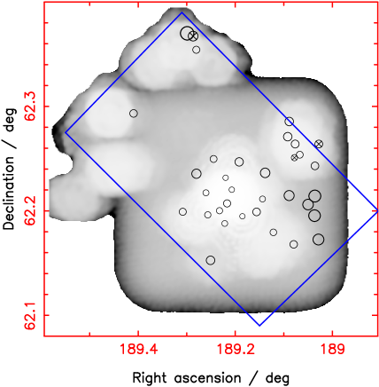
The GOODS-N region covers an area of approximately $10\times 16.5$ arcmin, centred on $12^{\rm{h}}36^{\rm{m}}55^{\rm{s}}$, $+62^{\circ}14\arcmin 15\arcsec$ (Giavalisco et al. 2004). All of the SCUBA data from several extensive imaging campaigns in the GOODS-N field have been combined into one sub-mm map, which we refer to as the ‘super-map’ (see Borys et al. 2003 and references therein). The resulting noise map and positions of extracted sources are displayed in Fig. 1. Since the super-map is a compilation of essentially all SCUBA data taken in the field, the associated noise map is extremely non-uniform. The most recent version of the GOODS-N super-map contains forty 850-$\mu$m sources detected above 3.5-$\sigma$ (Pope et al. 2005). From Monte Carlo simulations, we expect to find $\sim 3$ spurious sources in the extraction process (Borys et al. 2003). In order to refine our secure catalogue, we have explored the level of flux boosting (also referred to as Malmquist and/or Eddington bias) of these sources by applying the Bayesian approach discussed in Coppin et al. (2005). By simulating a distribution of pixel values, which depends on the chopping pattern, we determined the de-boosted flux for each of our sources. We then removed any sources from our sample which were severely affected by flux-boosting and possessed a non-negligible probability of having zero flux, which left us with 35 secure sub-mm sources. Note that the decision to reject sources due to likely flux boosting comes from a simple relationship based on signal and noise, and therefore it is easy to include the same criterion in our simulated sub-mm catalogues (discussed in Section 4.1).

Using the optical, radio and new Spitzer data in GOODS-N we have identified counterparts for all but one of the secure sub-mm sources (the details are discussed in Pope et al. 2006). The positions of the remaining 34 are plotted in Fig. 1. Spectroscopic redshifts are known for about half of the sub-mm catalogue; reliable photometric redshifts have been estimated for the remainder of the objects using the extensive optical and infra-red data (see Figure 1 of Pope et al. 2005 and Figure 7 of Pope et al. 2006). For those sub-mm sources possessing both spectroscopic and photometric redshifts, the standard deviation of $(z_{\rm phot}-z_{\rm spec})/(1+z_{\rm spec})$ is $0.10$.

The optical data for the GOODS-N region (Giavalisco et al. 2004), obtained with the Advanced Camera for Surveys (ACS) on-board the HST, has a uniform sensitivity within the boundaries indicated in Fig. 1, which represents the area studied in our cross-correlation analysis. We restricted our analysis to sources which are detected above 5-$\sigma$ and therefore, for all but the faintest magnitudes, we are far enough above the noise level that the subtle variations in exposure time will not affect our results. In addition to the 4 ACS bands ($B_{\rm{435}}$, $V_{\rm{606}}$, $i_{\rm{775}}$ and $z_{\rm{850}}$), the GOODS-N field has also been surveyed with several ground-based facilities, providing data in the following bands: U (KPNO, Capak et al. 2004); B, V, R, I, z (Subaru, Capak et al. 2004); and $J$, $K_{\rm{s}}$ (KPNO, Giavalisco et al. 2004). Using all of these optical data, photometric redshifts have been calculated for roughly half of the $\simeq 32{,}000$ optically-detected galaxies in GOODS-N. The accuracy of these photometric redshifts has been determined using the subset of sources (numbering $\simeq 1{,}700$) which also possess spectroscopic redshifts. The standard deviation of $(z_{\rm phot}-z_{\rm spec})/(1+z_{\rm spec})$ for the optical catalogue is 0.11. We note that throughout this paper we use AB magnitudes.

3 The cross-correlation function

The cross-correlation function $w_{\rm cross}(\theta)$ between two galaxy populations 1 and 2, in terms of an angular scale $\theta$, is defined as the fractional excess in the probability $\delta P$, relative to a random unclustered distribution, of finding both a galaxy of type 1 in a solid angle element $\delta\Omega_{1}$ and a galaxy of type 2 in a solid angle element $\delta\Omega_{2}$, separated by angle $\theta$:

$$\delta P=\Sigma_{1}\,\Sigma_{2}\,[1+w_{\rm cross}(\theta)]\,\delta\Omega_{1}\,\delta\Omega_{2},$$ (1)

where $\Sigma_{1}$ and $\Sigma_{2}$ are the surface densities of populations 1 and 2 (Peebles 1980).

The cross-correlation function $w_{\rm cross}(\theta)$ is measured from the galaxy distributions by constructing pair counts from the data-sets. A pair count between two galaxy populations 1 and 2, $D_{1}D_{2}(\theta)$, is a binned histogram of the separations $\theta$ of every galaxy of population 1 relative to all objects of population 2. In order to determine the cross-correlation function, fully incorporating the effects of the survey geometry and of statistical fluctuations, we must also generate random unclustered realizations of the galaxy distributions with the same angular selection functions as the real data. The pair counts between the data and random distributions (denoted $D_{i}R_{j}$) measure the actual average available area around each object, taking account of the survey window function and the distributions of the galaxies relative to the boundaries of the sample. In this way, we can construct correlation function estimators with the smallest bias and variance in the angular range under investigation.

The error in a correlation function estimator is determined from the variance of individual pair counts. It is important to note that, if a separation bin contains $N$ galaxy pairs, then the statistical variance in this bin will in general exceed the ‘Poisson error’ $\sqrt{N}$, even for an unclustered distribution of objects, as can be demonstrated by simulations or analytic calculations (e.g. Landy & Szalay 1993; Hamilton 1993; Bernstein 1994; Bernardeau et al. 2002). The increase in variance compared to the Poisson prediction depends on the survey geometry, but can be considerable for a sub-optimal estimator when the pair separation $\theta$ is not negligible compared to the survey dimensions. A fundamental cause of the excess non-Poisson variance is edge effects: the position of sources relative to the boundaries of the sample is important in determining the distribution of pair separations (i.e. a source distant $\theta_{0}$ from an edge is less likely to participate in pairs of separation $\theta>\theta_{0}$). The true variance of the correlation function estimator may be measured by techniques such as jack-knife re-sampling or Monte-Carlo simulations.

Various estimators for the cross-correlation function have been proposed. Two commonly used but (in general) sub-optimal estimators are:

$$w_{\rm cross}(\theta)=\frac{D_{1}D_{2}}{D_{2}R_{1}}-1;$$ (2)

$${\rm and}\ w_{\rm cross}(\theta)=\frac{D_{1}D_{2}}{D_{1}R_{2}}-1.$$ (3)

These two estimators are potentially biased, because in each case random realizations of only one of the two data-sets have been created, thus the statistical fluctuations and edge effects due to the distribution of sources in the other data-set have not been taken into account. Furthermore, equations 2 and 3 are not invariant when the indices $(1,2)$ are interchanged. In addition the variance of these estimators may significantly exceed the Poisson prediction, depending on the survey geometry (e.g. Landy & Szalay 1993). Better estimators for the cross-correlation function are:

$$w_{\rm cross}(\theta)=\frac{D_{1}D_{2}\times R_{1}R_{2}}{D_{1}R_{2}\times D_{2}R_{1}}-1;$$ (4)

$${\rm and}\ w_{\rm cross}(\theta)=\frac{D_{1}D_{2}-D_{1}R_{2}-D_{2}R_{1}+R_{1}R_{2}}{R_{1}R_{2}}.$$ (5)

These two estimators are modified versions of those originally suggested for the auto-correlation function by Hamilton (1993) and Landy & Szalay (1993), respectively. In each case statistical fluctuations in both data-sets have been incorporated, and the equations are symmetrical in the indices $(1,2)$.

4 Cross-correlation measurements

4.1 Generation of random catalogues

In order to measure the cross-correlation function robustly we must generate random (unclustered) comparison data-sets for each of our surveys, possessing the same angular selection functions as the survey data. For the optical observations, we generated random catalogues by uniformly populating the region delineated by the straight boundaries in Fig. 1. One of the 34 secure sub-mm counterparts lies outside the area of uniform optical sensitivity, as indicated in Fig. 1, and as a result was excluded from our analysis.

For the sub-mm data-set, we generated random distributions using the noise map plotted in Fig. 1. Firstly, candidate sources were randomly generated inside the analysis region from the flux distribution fitted to this sub-mm data-set by Borys et al. (2003):

$$N(S)\propto\left[\left(\frac{S}{S_{0}}\right)^{\alpha}+\left(\frac{S}{S_{0}}\right)^{\beta}\right]^{-1},$$ (6)

where $N(S)\,dS$ is the number of sources with fluxes between $S$ and $S+dS$. The best-fitting values of the parameters are approximately $\alpha=1$, $\beta=3.3$, and $S_{0}=1.8$ mJy. This distribution represents a number-counts slope steepening with increasing flux, and is a reasonable fit to all existing SCUBA data (although the detailed form of this function is not important – any function which fits the current data would suffice for our purpose). The candidate source was only retained if its signal-to-noise ratio determined by the noise map exceeded $3.5$ and if it satisfied the flux-deboosting criterion described in Section 2.

Secondly, we must take account of the angular resolution of the sub-mm observations, otherwise the highly non-uniform noise distribution will cause the deepest portions of the map to be over-populated by random sources in comparison to the real data. Although the beam size of the SCUBA instrument at $850\,\mu$m is about 15 arcsec, the sub-mm catalogue displays a dearth of pairs separated by less than 30 arcsec (compared to the number of pairs expected by random chance), owing to the difficulty of fitting very close pairs of sources in the extraction process. Therefore, we rejected a candidate random source if its putative position was closer than 30 arcsec to an existing random source with a higher signal-to-noise ratio. If the near neighbour possessed a lower signal-to-noise ratio than the candidate object, it was expunged from the random catalogue in favour of the new source. The final distributions of fluxes in our random catalogues were found to agree reasonably well with that observed for the real sub-mm data-set. The sub-mm catalogue plotted in Fig. 1 does in fact contain two pairs separated by less than 30 arcsec: for consistency, the source with the lowest signal-to-noise ratio was removed in each case, leaving us with a total of 31 sub-mm objects.

4.2 Determination of errors

As discussed in Section 3, the assumption of Poisson errors can be a poor approximation for the variance in a correlation function measurement. Moreover, this approach cannot establish the covariances between separation bins. A common technique for improving the error determination is jack-knife re-sampling, in which correlation functions are measured for many sub-samples of the data-sets in order to estimate the statistical fluctuations and covariance (e.g. Scranton et al. 2002). However, our sub-mm catalogue is too small to allow the reliable application of this method.

We therefore determined the covariance matrix of each correlation function measurement using Monte Carlo realizations, in which the actual data-sets were substituted by random realizations generated as described in Section 4.1. This is an acceptable approximation given that the angular clustering of these data-sets is weak compared to the shot noise error. Each mock realization of the data was analyzed by our correlation function pipeline, and the results for many realizations enabled the covariance matrix to be constructed.

4.3 Bias and variance of estimators

Fig. 2 indicates how the measured cross-correlation function depends on the estimator employed, analyzing a test case consisting of all 31 sub-mm sources and a bright $z$-filter magnitude slice of ACS galaxies ($20<m_{z}<22$). Throughout this paper we measure the cross-correlation function up to an angular scale of 5 arcmin in 10 bins of width $0.5$ arcmin. The plotted error bars always correspond to the diagonal elements of the covariance matrix measured as described in Section 4.2. The ‘good’ estimators for $w_{\rm cross}(\theta)$ (equations 4 and 5) produce mutually consistent results that display no evidence for cross-correlation. ‘Estimator 1’ (equation 2) displays a strong positive cross-correlation. ‘Estimator 2’ (equation 3) is unbiased for these distributions, but possesses a significantly increased variance.

Figure 2: The cross-correlation function of the SCUBA and ACS data-sets measured by a variety of estimators. In this test case we restricted the ACS sample to galaxies in the $z$-filter magnitude range $20<m_{z}<22$. Estimators 1 to 4 correspond to equations 2, 3, 4 and 5, respectively, whilst labels ‘1’ and ‘2’ in these equations refer to the optical and sub-mm data-sets, respectively. The errors are determined by Monte Carlo realizations. The separate measurements are offset along the $x$-axis for clarity.

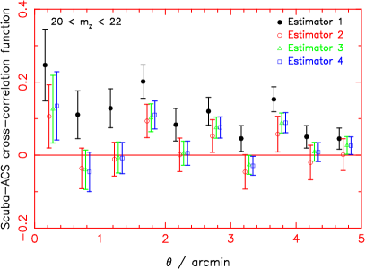
For ‘estimator 1’, which displays the strong bias in Fig. 2, we averaged over random optical data-sets, but not random sub-mm catalogues. This is problematic, because our actual sub-mm data-set (Fig. 1) happens by chance to have more sources in the lower half of the field than the average realization, accidently coinciding with an overdensity in the optical data-set. In terms of pair counts, $D_{\rm sub-mm}D_{\rm opt}$ is spuriously high in comparison to $D_{\rm sub-mm}R_{\rm opt}$, causing the positive offset in the cross-correlation function over a range of scales. We emphasize that this is purely an artefact of using a sub-optimal estimator – these large-scale fluctuations are entirely consistent with random realizations of the data-sets, but poor estimators can mistakenly assign significance to this.

In Fig. 3 we plot the ratio between the correlation function error determined by the Monte Carlo realizations and the Poisson error, as a function of scale for the four estimators. The ‘good’ estimators of equations 4 and 5 perform best in terms of variance as well as bias, approaching the Poisson prediction. ‘Estimator 2’ (equation 3) possesses a significantly larger variance than that predicted by Poisson statistics.

Figure 3: The standard deviation in the cross-correlation function of the SCUBA and ACS data-sets measured by a variety of estimators, as determined by Monte Carlo realizations. In this test case we analyzed the same sample of ACS galaxies as in Fig. 2, and estimators 1 to 4 have the same correspondences. The errors are normalized to the prediction for purely Poisson statistics.

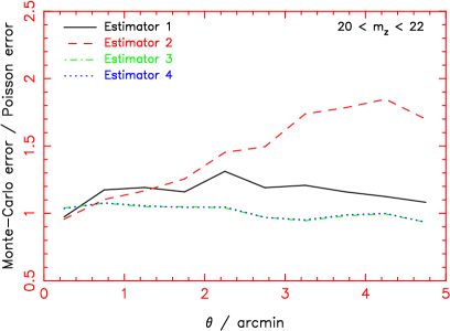
For the rest of this paper we chose to use the Landy-Szalay-based estimator for the cross-correlation function (equation 5, ‘estimator 4’). In all cases we determined the pair counts $D_{1}R_{2}$, $D_{2}R_{1}$ and $R_{1}R_{2}$ by averaging over 10 random catalogues, each containing the same number of galaxies as the real survey data-sets.

4.4 Attempted detection of cosmic magnification

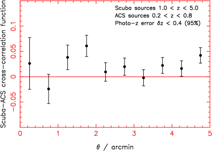
One potential source of genuine cross-correlation between our data-sets is gravitational lensing (‘cosmic magnification’) of background sub-mm sources by dark matter haloes traced by foreground optical galaxies; we investigate this effect first. In order to optimize any detection of cosmic magnification, we used the photometric redshift information to restrict our comparison to low-redshift ($0.2<z<0.8$) optical sources and high-redshift ($1<z<5$) sub-mm objects. We only utilized galaxies with ‘high-quality’ photometric redshifts with errors better than $\delta z=0.4$ ($95\%$ confidence limit, see Mobasher et al. 2004).

The result is plotted in Fig. 4. There is weak evidence that $w_{\rm cross}(\theta)$ is inconsistent with zero. In fact a small positive constant value $w\approx 0.02$ provides a good fit (using the full covariance matrix). However, we do not interpret this as evidence for an astrophysically-significant cross-correlation, given that the expected form of such a correlation is strongly scale-dependent (see Section 5). In contrast, any residual systematic problems – such as uncertainties in the underlying mean source density, the integral constraint correction for small fields, or unrecognised calibration fluctuations – would produce a small constant offset in the correlation function (e.g. Blake & Wall 2002).

Figure 4: Cross-correlation function of the SCUBA and ACS data-sets, measured for samples selected in a manner which should be efficient for the detection of cosmic magnification. The measurements contain weak evidence for a small positive constant offset from zero, but we do not interpret this as an astrophysically-significant cross-correlation, as explained in the text.

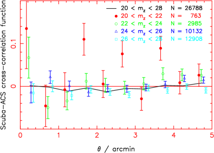
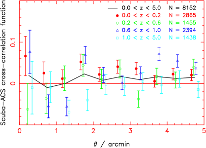
Exploring further, we also measured the cross-correlation function between all SCUBA sources and various sub-samples of the ACS galaxies. Fig. 5 displays the results measured in different magnitude bands. Fig. 6 plots the measurements in redshift bands, only including those ACS galaxies with high-quality photometric redshifts. In no case do we find a significant detection of a cross-correlation (that cannot be fit by a small constant offset). We also detected no significant cross-correlation by varying the flux threshold of the sub-mm galaxies. Bright ($S_{850\mu{\rm m}}>10$ mJy) sub-mm sources are expected to have the steepest flux distribution and hence the strongest cross-correlation. However, the number of such sources in our sample is very small.

Figure 5: Cross-correlation function of the SCUBA and ACS data-sets, measured in $z$-filter magnitude intervals of the ACS sources. The solid line is the cross-correlation result using the whole optical sample. The separate measurements are offset along the $x$-axis for clarity.

Figure 6: Cross-correlation function of the SCUBA and ACS data-sets, measured in redshift bands of the ACS sources. The solid line is the cross-correlation result using the whole optical sample. Only optical galaxies with ‘high-quality’ photometric redshifts are included in the analysis. The separate measurements are offset along the $x$-axis for clarity.

4.5 Attempted detection of galaxy clustering

The second potential source of genuine cross-correlation between our data-sets is galaxy clustering, which would arise if the sub-mm and optical objects traced the same population of dark matter haloes in the case of overlapping redshift distributions. In order to efficiently search for clustering we again used the photometric redshift information, firstly restricting our data-sets to galaxies with high-quality photometric redshifts as defined above. We also limited the input sub-mm and optical data-sets to the redshift range $0.8<z<2.0$ in order to maximize the overlap of the catalogues. We then measured the pair counts in angular separation bins, weighting each galaxy pair by a factor depending on its redshift difference $\delta z=z_{1}-z_{2}$:

$${\rm Weight}=\exp{\left[-\frac{1}{2}\left(\frac{\delta z}{C}\right)^{2}\right]},$$ (7)

where $C=0.1$ (determined empirically to optimize the signal-to-noise ratio of the measurement). These weights strongly increase the contribution of pairs at similar redshifts, optimizing any detection of mutual clustering. The cross-correlation function was then determined using the usual combination of the (weighted) pair counts. The redshifts of sources in the random comparison catalogues were assigned by randomizing the redshifts of the real data. The error in the correlation function was determined using Monte Carlo realizations, as before.

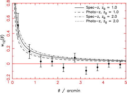
The result is plotted as the solid circles in Fig. 7, and shows evidence for a positive correlation on small scales. Fitting a power-law model $w(\theta)=A\,\theta^{-1}$ to the result allows us to reject a model with no correlation ($A=0$) with a significance level of $3.5$-$\sigma$. The slope of $1.0$ was determined by fitting a power law to the higher signal-to-noise auto-correlation function of the ACS galaxies, as described below, and provides a better fit than the canonical slope of $0.8$. We checked that adding data with lower-quality photometric redshifts or changing the value of $C$ in equation 7 did not improve the significance of the detection.

Figure 7: The solid circles plot the cross-correlation function of the SCUBA and ACS data-sets, measured in a manner designed to optimize any detection of galaxy clustering. The open circles display a measurement of the same statistic for an auto-correlation function of the ACS galaxies. The lines represent the best fits of a power-law model $w(\theta)=A\,\theta^{-1}$ to separations in the range $\theta<3$ arcmin.

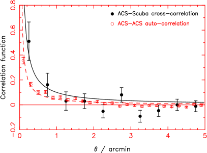
For comparison, we repeated the calculation analyzing the clustering of the ACS galaxies alone via an auto-correlation function, weighting galaxy pairs as before. The result, plotted as the open circles in Fig. 7, can be established with greater significance, owing to the larger optical sample. The auto-correlation amplitude appears to be lower than the cross-correlation amplitude on the smallest scales (the significance of the offset is 2-$\sigma$). A tentative interpretation of this finding would be the expected higher clustering bias of sub-mm galaxies. This is consistent with suggestions of clustering of sub-mm galaxies in redshift-space (Blain et al. 2004). We note that differences in the redshift distributions of the sub-mm and optical sources will affect this comparison: the ACS catalogue contains more objects at the lower end of the redshift range analyzed. However, for these low-redshift pairs a given angular scale corresponds to a smaller physical scale, which will boost the correlation amplitude. Therefore, the 2-$\sigma$ significance of the discrepancy between the cross-correlation and auto-correlation functions in Fig. 7 is conservative.

There are several ways in which one might try to refine this procedure, including: changing the weighting scheme for SCUBA galaxies which have spectroscopic redshifts; adapting the weight of each pair depending on the quality of the photometric redshift(s); using cuts on colour as well as magnitude; etc. We have not performed an exhaustive investigation of these issues, since what is really required to achieve definitive measurements is larger sub-mm surveys, as discussed in Section 6.

5 Cross-correlation modelling

5.1 Cosmic magnification prediction

In Section 4.4 we failed to detect any evidence for cross-correlation between our sub-mm and optical data-sets of the form which might be induced by cosmic magnification. We now compare this result to theoretical predictions for the size of this effect.

The magnitude of the cross-correlation amplitude induced by cosmic magnification is determined in part by the slope of the differential number-counts for the background population: $w_{\rm cross}\propto(\beta-1)$, where the number of sources with fluxes between $S$ and $S+dS$ is given by $S^{-\beta}\,dS$. The number-counts slope for bright sub-mm sources is known to be exceptionally steep, $\beta\simeq 3$, increasing the effect of cosmic magnification relative to populations with more shallow counts (such as quasars, where the maximum slope $\beta\simeq 2$ is only reached for the very brightest sources, Scranton et al. 2005). For fainter sub-mm galaxies the effective value of $\beta$ becomes smaller, in accordance with equation 6.

The cross-correlation function due to cosmic magnification can be predicted using simple models (e.g. Moessner & Jain 1998). If we assume that the source and lens populations are at fixed redshifts $z_{\rm s}$ and $z_{\rm l}$, then

$$w_{\rm sl}(\theta)=\frac{3\Omega_{\rm m}(\beta-1)}{2\pi L_{\rm H}^{2}}\frac{b_{\rm l}g_{\rm ls}}{a(z_{\rm l})}\int kP(k,z_{\rm l})J_{0}(kx(z_{\rm l})\theta)dk,$$ (8)

where $\Omega_{\rm m}$ is the present-day matter density relative to the critical density, $L_{\rm H}\equiv c/H_{0}$ is the Hubble length in units of $h^{-1}$ Mpc, $b_{\rm l}$ is the linear biassing factor for the lenses, $g_{\rm ls}=x(z_{\rm l})[x(z_{\rm s})-x(z_{\rm l})]/x(z_{\rm s})$ is the geometrical factor for lensing, $x(z)$ is the co-moving angular diameter distance for a flat Universe, $a(z)$ is the usual cosmological scale factor, $P(k,z)$ is the matter power spectrum at redshift $z$ (including non-linear clustering), and $J_{0}(u)$ is the zeroth-order Bessel function. In equation 8 the units of $x(z)$, $k$ and $P(k,z)$ are $h^{-1}$Mpc, $h\,{\rm Mpc}^{-1}$ and $h^{-3}\,{\rm Mpc}^{3}$, respectively.

We considered a foreground lens population with $b_{\rm l}=1$ at $z_{\rm l}=0.5$ and a background source population at $z_{\rm s}=2$. We assumed a spatially-flat cosmology with cosmological parameters $\Omega_{\rm m}=0.3$ and $H_{0}=70$ km s^-1 Mpc^-1, and generated a non-linear power spectrum using the prescription of Peacock & Dodds (1994), using a linear power spectrum produced from the fitting formulae of Eisenstein & Hu (1998), with baryon fraction $\Omega_{\rm b}/\Omega_{\rm m}=0.15$, spectral index $n_{\rm s}=1$ and zero-redshift normalization $\sigma_{8}=0.8$ (scaled to redshift $z_{\rm l}$ using the linear growth factor of Carroll, Press & Turner 1992). In Fig. 8 we plot the resulting cross-correlation function of equation 8 for number-count slopes between $\beta=2.0$ and $\beta=3.0$. Realistically, the redshift distributions of the background and foreground populations will be broader than the infinitesimal shells we have assumed; this will lower the amplitude of the cross-correlation, owing to the geometrical factor $g_{\rm ls}$ in equation 8.

Figure 8: Model cross-correlation function for cosmic magnification of a background source population at $z_{\rm s}=2$ by a foreground lens population at $z_{\rm l}=0.5$. Different curves correspond to different slopes $\beta$ of the number-counts relation for the background population. The plotted data points are a reproduction of our measurement from Fig. 4.

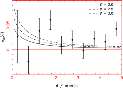
As can be seen, the predictions of Fig. 8 provide an entirely acceptable fit to the null measurement of cosmic magnification plotted in Fig. 4 (which is reproduced in Fig. 8 for comparison). However, our results appear to disagree somewhat with those of Almaini et al. (2005, Figures 1 and 2), who observed a significantly higher cross-correlation amplitude between sub-mm and optically-selected galaxies, with their favoured explanation being lensing magnification. The signal-to-noise of the measurements is low, but we find it difficult to reconcile these results, corresponding to $w_{\rm sl}\simeq 0.2$ on small scales $\theta\simeq 30\arcsec$, with our lensing model – unless the fields studied happen to contain a highly dis-proportionate concentration of massive lenses.

As an alternative and cruder model, we can estimate the quantity of lenses required to generate a given cross-correlation signal by assuming a simple distribution of singular isothermal spheres. Denoting the lensing magnification factor as $\mu$, the enhancement in surface density of background sources is given by $\mu^{\beta-1}$, where $\beta$ is the slope of the differential number counts distribution (as defined above). For a background source at (lensed) angular separation $\theta$ from an isothermal lens with Einstein radius $\theta_{\rm E}$,

$$\mu=\left(1-\frac{\theta_{\rm E}}{\theta}\right)^{-1}$$ (9)

(Bartelmann & Schneider 2001, equation 3.19). Assuming $\beta=3$ (which is appropriate for the brightest SCUBA galaxies), a correlation function $w(0.5\arcmin)\simeq 0.2$ is generated if sources have an average magnification such that $w\simeq\mu^{\beta-1}-1$ or $\mu\simeq 1.1$. Using equation 9, the average source must be at angular separation $\theta=0.5$ arcmin from a lens with Einstein radius $\theta_{\rm E}\simeq 2.6\arcsec$. The Einstein radius of an isothermal sphere with 1D velocity disperson $\sigma_{v}$ is given by

$$\theta_{\rm E}=4\pi\left(\frac{\sigma_{v}}{c}\right)^{2}\left[\frac{x(z_{\rm s})-x(z_{\rm l})}{x(z_{\rm s})}\right]$$ (10)

(Bartelmann & Schneider 2001, equation 3.17). Substituting the approximate value $0.5$ for the geometrical factor, we obtain $\theta_{\rm E}\simeq(0.6\arcsec)(\sigma_{v}/200{\rm\,km\,s}^{-1})^{2}$. Hence in this simple model, lenses of velocity dispersion $\sigma_{v}\simeq 420$ km s^-1 (i.e., galaxy groups) must be responsible for the lensing magnification. Given that our background sources must be located on average $0.5$ arcmin from these lenses, we estimate that a lens surface density $\simeq 1$ arcmin^-2 is required. This is consistent with the density of optical sources at the relevant magnitude limit, but significantly exceeds the expected density of groups (i.e., $\simeq 0.02$ arcmin^-2, e.g. Yan et al. 2004). We conclude that the fields observed by Almaini et al. (2005) would have to be unusual areas of sky in order to generate an angular correlation function $w(0.5\arcmin)\simeq 0.2$ by lensing magnification. We note that if $w(0.5\arcmin)=0.04$ (Fig. 8), then the equivalent lens velocity dispersion is $\sigma_{v}\simeq 200$ km s^-1, more typical of individual galaxies with a surface density $\simeq 1$ arcmin^-2 in the appropriate redshift range.

As suggested by Almaini et al., an alternative explanation for their observed cross-correlations is that a higher-than-expected fraction of the sub-mm galaxies studied were located at relatively low redshifts, $z\la 1$, and that the signal was generated by galaxy clustering rather than by lensing magnification, as discussed in Section 5.2 below. However, only $\sim 10\%$ of our sample of sub-mm sources in GOODS-N lies at $z<1$, and we note that, in surveys with large redshift depth, it is difficult to generate any significant angular cross-correlation amplitude from galaxy clustering without photometric redshift information to restrict the redshift slices compared.

5.2 Galaxy clustering prediction

We now estimate the amplitude of angular cross-correlation resulting from the mutual clustering of sub-mm and optically-selected galaxies with similar photometric redshifts. Both populations trace the underlying distribution of dark matter, which (for the purposes of this calculation) we will assume is clustered in accordance with a power-law spatial auto-correlation function, $\xi(r)=(r/r_{0})^{-\gamma}$, where $r$ is a co-moving separation, $r_{0}$ is the co-moving ‘clustering length’ at the redshift in question, and the slope $\gamma=1.8$. We will further assume that the two galaxy populations are linearly biased with respect to the dark matter fluctuations, possessing clustering lengths $r_{1}$ and $r_{2}$. In this case, using the definition of bias, the spatial cross-correlation function $\xi_{\rm cross}$ is derived by replacing $r_{0}$ with $(r_{1}r_{2})^{1/2}$ in the formula for $\xi(r)$. The spatial cross-correlation function, $\xi_{\rm cross}(r)$, must then be projected onto an angular cross-correlation function, $w_{\rm cross}(\theta)$.

We consider the two cases of sub-mm galaxies with spectroscopic redshifts and with only photometric redshifts. These are compared with an optical photo-$z$ catalogue. In the first case, the contribution from each sub-mm galaxy (at redshift $z=z_{0}$) to the angular cross-correlation at angle $\theta$ can be determined by integrating $\xi_{\rm cross}$ along the line-of-sight at angular separation $\theta$, weighted by the redshift probability distribution $p(z)$ of the optically-selected sources (normalized such that $\int p(z)\,dz=1$), i.e.

$$w_{\rm cross} = \int p(z)\,\xi_{\rm cross}(\theta,z)\,dz$$ (11)

$$\simeq (r_{1}r_{2})^{\gamma/2}\int p(z)\,[(x_{0}\theta)^{2}+(x-x_{0})^{2}]^{-\gamma/2}dz,$$

where $x(z)$ is the co-moving radial co-ordinate and $x_{0}\equiv x(z_{0})$. The redshift distribution $p(z)$ is the error distribution of the photometric redshifts for optical galaxies with best-fitting redshifts near $z=z_{0}$. We will assume that this function is a Gaussian distribution with mean $z_{0}$ and standard deviation $\sigma_{z}$. As the width of this function is much larger than the clustering length, a good approximation for equation 11 is

$$w_{\rm cross}=C_{\gamma}(r_{1}r_{2})^{\gamma/2}p(z_{0})\left(\frac{dx}{dz}(z_{0})\right)^{-1}x(z_{0})^{1-\gamma}\theta^{1-\gamma},$$ (12)

where $C_{\gamma}=\Gamma(\frac{1}{2})\,\Gamma{(\frac{\gamma}{2}-\frac{1}{2}})/\Gamma(\frac{\gamma}{2})$.

For the case where the sub-mm source redshift is only photometric, in order to obtain the resulting angular cross-correlation we must integrate equation 12 over redshift again, weighting by a further factor of $p(z)$. Hence we assume (for the purposes of this calculation) that the photometric redshift error distribution for the sub-mm galaxies is the same as for the optical sources. The result is an extra damping of the cross-correlation amplitude:

$$w_{\rm cross}=C_{\gamma}(r_{1}r_{2})^{\gamma/2}\theta^{1-\gamma}\int p(z)^{2}\left(\frac{dx}{dz}\right)^{-1}x(z)^{1-\gamma}dz.$$ (13)

Equation 13 is in fact the usual Limber equation for the projection of spatial clustering (e.g. Peebles 1980).

In order to evaluate these expressions, we take a photometric-redshift error $\sigma_{z}=0.2$, which is characteristic of our data (i.e. $\sigma_{z}/(1+z)\simeq 0.1$ as noted in Section 2). We assume that the co-moving clustering length of the optically-selected galaxies is constant with redshift (Lahav et al. 2002), $r_{1}=5\,h^{-1}$ Mpc, and take an enhanced clustering amplitude for the sub-mm galaxies, $r_{2}=7\,h^{-1}$ Mpc (Blain et al. 2004). The predictions of equations 12 and 13 for the cases of spectroscopic and photometric redshifts for the sub-mm galaxies are displayed in Fig. 9 for $z_{0}=1$ and $z_{0}=2$. Finally, we make the approximation that each sub-mm galaxy is an independent probe of the clustering, thus the angular correlation functions determined for each sub-mm source (which may have a spread as indicated in Fig. 9) can simply be averaged. Since approximately half of the sub-mm galaxies have spectroscopic redshifts, the final result should fall somewhere in between the curves shown in Fig. 9. This model is a reasonable fit to our observations, which are also reproduced in Fig. 9 for comparison.

Figure 9: Model cross-correlation function generated by the mutual clustering of sub-mm and optically-selected galaxies. We compare cases where the sub-mm galaxy redshift $z_{0}$ is known with spectroscopic and photometric accuracy, for $z_{0}=1$ and $z_{0}=2$. We assume that the optical galaxies always have a photometric redshift distribution centred at $z_{0}$ with an r.m.s. width $\sigma_{z}=0.2$. The plotted data points are a reproduction of our measurement from Fig. 7.

6 Prospects for future surveys

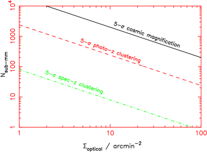
In order to measure the cosmic magnification pattern with reasonable accuracy (say, signal-to-noise exceeding 3 in several separation bins) we require cross-correlation function measurements with precision $\delta w\sim 0.002$ in bins of width $\delta\theta\sim 0.5$ arcmin (see Fig. 8). The error in the correlation function is, roughly speaking, determined by the number of galaxy pairs measured: $\delta w\sim N_{\rm pairs}^{-1/2}$ (with the caveats discussed in Section 3). If $\Sigma_{\rm opt}$ is the surface density of optical galaxies in the appropriate redshift range, then each sub-mm source participates in an average of $\Sigma_{\rm opt}\times 2\pi\theta\,\delta\theta$ pairs in a bin of average separation $\theta$.

For the current cosmic magnification analysis (Fig. 4), we have a surface density of optical sources $\Sigma_{\rm opt}\simeq 10$ arcmin^-2 in the appropriate redshift range ($0.2<z<0.8$). Since $N_{\rm sub-mm}\simeq 30$, we recover $\delta w\simeq 0.03\times\theta{\rm(arcmin)}^{-1/2}$ in bins of width $\delta\theta=0.5$ arcmin, as observed in Fig. 4. In order to achieve a measurement of cosmic magnification with reasonable significance we therefore require a sub-mm survey with $\sim 100$ times as many sources. This should easily be achieved with surveys being planned with the new SCUBA-2 instrument (Holland et al. 2003). However, it is worth bearing in mind that a high density of optical galaxies and reasonably good photo-$z$ estimates will be required.

The cross-correlation resulting from the mutual clustering of sub-mm and optically-selected galaxies should be easier to detect, owing to its larger amplitude (Fig. 9). Let us assume optical data of equivalent quality to that used in this study. The surface density of optical galaxies with ‘high-quality’ photometric redshifts in a redshift range overlapping with the sub-mm sources is again $\Sigma_{\rm opt}\simeq 10$ arcmin^-2, which we divide into 3 independent photo-$z$ bins. Since $N_{\rm sub-mm}\simeq 15$ in the region of overlap, we recover $\delta w\simeq 0.08\times\theta{\rm(arcmin)}^{-1/2}$ in bins of width $\delta\theta=0.5$ arcmin. However, the expected amplitude of the cross-correlation due to clustering (Fig. 9) is significantly larger than that due to cosmic magnification (Fig. 8): $w_{\rm cross}\simeq 0.1-0.2$ at $\theta=1$ arcmin. We therefore conclude that a sub-mm survey with $\sim 10$ times as many sources as used in the current study should suffice to measure this signal with reasonable accuracy, assuming an appropriate quantity of optical follow-up. This should be achievable for the on-going SHADES project (Mortier et al. 2005). Alternatively, we note that the clustering amplitude could be accurately measured using the current catalogues if spectroscopic redshifts were available for both the optical and sub-mm sources. Figure 10 illustrates the accuracy of measurement achievable for each type of analysis through the comparison of sub-mm and optical catalogues.

Figure 10: A rough indication of the accuracy with which sub-mm surveys yielding $N_{\rm sub-mm}$ sources can measure cosmic magnification and galaxy clustering through comparison with deep optical catalogues with surface density $\Sigma_{\rm opt}$. The 5-$\sigma$ threshold for each type of analysis is defined using estimates for the cross-correlation function amplitude and error within an assumed range of measured scales. The amplitudes are obtained from the correlation function models developed in Section 5. The errors are derived from the number of object pairs within the separation bin, assuming a Poisson error $\delta w=N_{\rm pairs}^{-1/2}$. For the cosmic magnification analysis, we assume $w(\theta)=0.02$ at a scale $\theta=1$ arcmin (Fig. 8) and consider a bin of width $\delta\theta=0.5$ arcmin. For the photo-$z$ clustering measurement we use the same separation bin, but assume $w(1\,{\rm arcmin})=0.1$ (Fig. 9) and divide the catalogues into three independent photo-$z$ bins. For the estimate where all objects have spectroscopic redshifts, we spread the optical sources over a redshift range $1<z<2$ and consider the measurement of a spatial correlation function $\xi=1$ at a scale $5\,h^{-1}$ Mpc in a bin of width $1\,h^{-1}$ Mpc.

7 Summary

We have investigated the cross-correlation between sub-mm and optical sources in the GOODS-N survey region, using photometric redshift information. We find that:

• Comparing high-redshift $(z>1)$ SCUBA sources with low-redshift $(0.2<z<0.8)$ optical galaxies, we can detect no evidence for cross-correlation due to cosmic magnification. We attribute previous reported detections to either: (1) a difference in the correlation function estimator employed; (2) analysis of a field that happens to contain a highly dis-proportionate concentration of massive lenses; or (3) a higher-than-expected fraction of sub-mm galaxies residing at relatively low redshifts $z\la 1$. Based on calculations of the expected amplitude of the lensing magnification signal in the standard cosmology, the sub-mm data-set must be increased in size by a factor $\simeq 100$ to secure a significant measurement.

• Comparing optical and sub-mm sources in identical photometric redshift slices, we detect evidence for a cross-correlation due to galaxy clustering (with a significance level of $3.5$-$\sigma$). The sub-mm sources appear to possess a higher bias factor than the optical galaxies (with a significance of 2-$\sigma$). This observation, if confirmed by larger surveys, would support the hypothesis that sub-mm sources form in relatively dense environments in the high-redshift Universe.

One of the primary goals of the SHADES project (Mortier et al. 2005) is to measure the clustering properties of sub-mm galaxies via an auto-correlation function analysis. We note that the cross-correlation with optically-selected galaxies could also provide valuable information (owing to the higher surface density of optical sources), provided that the optical data are of sufficient quality. Cross-correlation in different redshift slices, in order to measure the lensing magnification, is an independent effect which should add an extra structure formation diagnostic to future sub-mm surveys, such as those that will be carried out with SCUBA-2. In terms of structure formation models, the auto- and cross-correlation functions have a different dependence on the halo occupation distribution, as well as on redshift and other source properties. Hence, an investigation of cross-correlation in future ambitious sub-mm surveys holds the promise of unravelling details of galaxy formation and bias within massive haloes.

References

- [1] Almaini O. et al., 2003, MNRAS, 338, 303
- [2] Almaini O., Dunlop J.S., Willott C.J., Alexander D.M., Bauer F.E., Liu C.T., 2005, MNRAS, 858, 875
- [3] Bartelmann M., Schneider P., 2001, Physics Reports, 340, 291
- [4] Baugh C.M., Lacey C.G., Frenk C.S., Granato G.L., Silva L., Bressan A., Benson A.J., Cole S., 2005, MNRAS, 356, 1191
- [5] Bernardeau F., Colombi S., Gaztanaga E., Scoccimarro R., 2002, PhR, 367, 1
- [6] Bernstein G., 1994, ApJ, 424, 569
- [7] Blain A.W., Smail I., Ivison R.J., Kneib J.-P., Frayer D.T., 2002, PhR, 369, 111
- [8] Blain A.W., Chapman S.C., Smail I., Ivison R., 2004, ApJ, 611, 725
- [9] Blake C., Wall J., 2002, MNRAS, 337, 993
- [10] Borys C., Chapman S., Halpern M., Scott D., 2002, MNRAS, 330, 92
- [11] Borys C., Chapman S., Halpern M., Scott D., 2003, MNRAS, 344, 385
- [12] Borys C., Scott, D., Chapman S., Halpern M., Nandra K., Pope A., 2004, MNRAS, 355, 485
- [13] Capak P. et al., 2004, AJ, 127, 180
- [14] Carroll S.M., Press W.H., Turner E.L., 1992, ARA&A, 30, 499
- [15] Chapman S.C., Blain A.W., Smail I., Ivison R.J., 2005, ApJ, 622, 772
- [16] Coppin K., Halpern M., Scott D., Borys C., Chapman S., 2005, MNRAS, 357, 1022
- [17] Eisenstein D.J., Hu W., 1998, ApJ, 496, 605
- [18] Giavalisco M. et al., 2004, ApJ, 600, L93
- [19] Hamilton A.J.S., 1993, ApJ, 417, 19
- [20] Holland W.S. et al., 1999, MNRAS, 303, 659
- [21] Holland W.S., Duncan W., Kelly B.D., Irwin K.D., Walton A.J., Ade P.A.R., Robson E.I., 2003, SPIE, 4855, 1
- [22] Ivison R.J. et al., 2002, MNRAS, 337, 1
- [23] Lahav O. et al., 2002, MNRAS, 333, 961
- [24] Landy S.D., Szalay A.S., 1993, ApJ, 412, 64
- [25] Mobasher et al., 2004, ApJ, 600, L167
- [26] Moessner R., Jain B., 1998, MNRAS, 294, 18
- [27] Mortier A.M.J. et al., 2005, MNRAS, 363, 563
- [28] Peacock J.A., Dodds S.J., 1994, MNRAS, 267, 1020
- [29] Peebles P.J.E., 1980, The Large-Scale Structure of the Universe, Princeton Univ. Press, Princeton, NJ
- [30] Percival W.J., Scott D., Peacock J.A., Dunlop J.S., 2003, MNRAS, 338, L31
- [31] Pope A., Borys C., Scott D., Conselice C., Dickinson M., Mobasher M., 2005, MNRAS, 358, 149
- [32] Pope A. et al., 2006, MNRAS, submitted
- [33] Scranton R. et al., 2002, ApJ, 579, 48
- [34] Scranton R. et al., 2005, ApJ, 633, 589
- [35] Scott S.E. et al., 2002, MNRAS, 331, 817
- [36] van Kampen E. et al., 2005, MNRAS, 359, 469
- [37] Yan R., White M., Coil A., 2004, ApJ, 607, 739