Galaxy cluster mass profiles

Abstract

Accurate measurements of the mass distribution in galaxy and cluster halos are essential to test the cold dark matter (CDM) paradigm. The cosmological model predicts a universal shape for the density profile in all halos, independent of halo mass. Its profile has a ‘cuspy’ centre, with no evidence for the constant density core. In this paper we carry out a careful analysis of twelve galaxy clusters, using Chandra data to compute the mass distribution in each system under the assumption of hydrostatic equilibrium. Due to their low concentration, clusters provide ideal objects for studying the central cusps in dark matter halos. The majority of the systems are consistent with the CDM model, but 4 objects exhibit flat inner density profiles. We suggest that the flat inner profile found for these clusters is due to an underestimation of the mass in the cluster centre (rather than any problem with the CDM model), since these objects also have a centrally peaked gas mass fraction. We discuss possible causes for erroneously low mass measurements in the cores of some systems.

1 Introduction

In hierarchical collapse models, $N$-body simulations predict a universal shape for the mass distribution in dark matter halos from dwarf galaxies (10⁷ M_⊙) to massive clusters (10¹⁵ M_⊙), independent of the value of the cosmological parameters. The density profile differs strongly from a simple single power-law, predicted in early theoretical work (Gunn & Gott, 1972; Fillmore & Goldreich, 1984; Hoffman & Shaham, 1985; White & Zaritsky, 1992), and is centrally concentrated with an inner cusp $\rho(r)\propto r^{-\alpha}$. The universality of the structure of dark matter halos formed through hierarchical clustering was ‘discovered’ in simulations performed by Navarro et al. (1995, 1996, 1997), hereafter NFW. In these early studies, an inner slope with $\alpha=1.0$ provided the best-fit to the spherically averaged density profiles. This was supported by various authors (Cole & Lacey, 1996; Tormen et al., 1997; Kravtsov et al., 1997). Later simulations at higher resolution indicated a steeper central cusp, with $\alpha=1.5$ (Fukushige & Makino, 1997, 2001, 2003; Moore et al., 1999; Ghigna et al., 2000; Klypin et al., 2001). A density profile similar to the NFW profile, but with $\alpha=1.5$ was suggested by Moore et al. (1999), hereafter M99.

A thorough understanding of the predictions made by simulations is essential in order to test the cold dark matter (CDM) paradigm against observations. There are several issues which need to be addressed by simulators, in particular in the high density central regions of halos where large numbers of particles and fine time resolution are required. In recent work there has been some debate over the form of the profile at the innermost resolved radii ($r<0.01r_{\rm vir}$). Power et al. (2003), Hayashi et al. (2003) and Navarro et al. (2004) suggest that the inner density profile does not converge to a well-defined power-law, but continues to flatten inwards. Diemand et al. (2005), on the other hand, dispute this result, continuing to support the existence of a central asymptotic power-law to the density profiles.

A further issue which remains unresolved numerically is the universality of the core profile. Jing & Suto (2000), for example, find that the inner slope steepens with decreasing halo mass. In addition, using analytical arguments, Hoffman & Shaham (1985) and Syer & White (1998) show that the halo profile should depend on the power spectrum of initial density fluctuations, with an inner slope given by $3(n+3)/(n+4)$ and $3(n+3)/(n+5)$, respectively, where $n$ is the power-law index of the spectrum.

Nevertheless, there are two robust predictions made by simulations which may be tested against observations: the density profile in CDM halos differs strongly from a single power-law, and the inner region is cuspy with a power-law slope in the range $1.0\lesssim\alpha\lesssim 1.5$ down to at least 1 per cent of the virial radius. In this paper we obtain mass profiles under the assumptions of hydrostatic equilibrium and spherical symmetry for a sample of X-ray peaked galaxy clusters using Chandra data. Straightforward deprojection techniques are robust and work well on such clusters. In addition, clusters halos have smaller concentrations than galaxies, making them ideal objects to study cusps. Work on the inner density slope of clusters of galaxies has also been carried out in recent studies by Katayama & Hayashida (2004), Arabadjis et al. (2004) and Pointecouteau et al. (2005).

A $\Lambda$CDM cosmology with $\Omega_{\rm\Lambda}=0.7$ and $h=0.7$ is adopted.

2 Cluster sample

The cluster sample used is listed in Table 1. Observations of objects with known short central cooling times, indicating a relatively relaxed object, were obtained from the Chandra archive. The sample of 12 objects was chosen to cover a range in cluster redshift ($z=0.02-0.46$) and ICM temperature ($k_{\rm B}T=2-15\rm\thinspace keV$). High redshift clusters observed by Chandra tend to be hotter, and in this sense the sample is not statistically complete; however, this will not in general affect the analyses carried out, and any biases introduced by the limited sample are discussed where relevant.

Data processing was carried out using the CIAO (Chandra Interactive Analysis of Observations) software package available from the CXC (Chandra X-ray Centre). Level 2 events files were updated to include the latest calibration. Only those X-ray events with ASCA grade classifications 0, 2, 3, 4 and 6 were included in the cleaned data set. Further screening was carried out to remove time intervals contaminated by background flares. The lightcurves were analysed using the script lc_clean written by M. Markevitch and provided by the CXC. The observation length remaining after screening (GTI; good time interval) is listed for each object in Table 1.

Cluster	Redshift	Obs. date	Exps. time		GTI		Emission peak (J2000)		$D_{\rm L}$		$D_{\rm A}$
			(ks)		(ks)		RA	Dec	(Mpc)		(kpc arcsec-1)
Abell 3112	0.0750	2001 Sep 15	17.	1	13.	5	03 17 57.7	$-$44 14 16.9	335.	2	1.4
2A 0335$+$096	0.0347	2000 Sep 06	20.	0	18.	1	03 38 40.6	$+$09 58 11.0	140.	6	0.7
Abell 478	0.0880	2001 Jan 27	42.	9	38.	9	04 13 25.2	$+$10 27 53.9	396.	9	1.6
PKS 0745$-$191	0.1028	2001 Jun 16	17.	9	14.	6	07 47 31.2	$-$19 17 38.8	468.	5	1.9
RXJ 1347.5$-$1145(1)	0.4510	2000 Mar 5	9.	1	8.	0	13 47 30.5	$-$11 45 09.5	2492.	9	5.7
RXJ 1347.5$-$1145(2)	0.4510	2000 Apr 29	10.	1	7.	2	13 47 30.5	$-$11 45 09.5	2492.	9	5.7
Abell 1795	0.0632	2000 Mar 21	19.	7	15.	6	13 48 52.5	$+$26 35 37.8	280.	0	1.2
Abell 1835	0.2523	1999 Dec 11	19.	8	18.	9	14 01 01.9	$+$02 52 43.4	1262.	4	3.9
Abell 3581	0.0218	2001 Jun 07	7.	3	6.	0	14 07 29.8	$-$27 01 04.2	93.	6	0.4
Abell 2029	0.0767	2000 Apr 12	19.	9	19.	8	15 10 56.1	$+$05 44 40.6	343.	2	1.1
RXJ 1532.9$+$3021	0.3615	2001 Aug 26	9.	5	6.	2	15 32 53.8	$+$30 20 58.5	1916.	3	5.0
MS 2137.3$-$2353	0.3130	2000 Dec 10	44.	2	19.	5	21 40 15.2	$-$23 39 39.9	1618.	8	4.7
Sersic 159$-$03 (AS 1101)	0.0564	2001 Aug 13	10.	1	9.	8	23 13 58.3	$-$42 43 35.0	248.	7	1.1

Table 1: Summary of the Chandra observations. Cluster redshift, observation date, exposure time, good time interval, X-ray emission peak, luminosity distance and angular scale. Both observations available for RXJ 1347.5$-$1145 were used.

3 Spectral analysis

3.1 Extracting spectra

For the spectral analysis, each cluster was divided into circular annuli around the X-ray emission peak, with strong point sources identified by eye and masked out. Regions disturbed by, for example, merging subclusters and radio lobes, were also removed (see Section 3.4). A spectrum was extracted for each annulus using the CIAO dmextract tool. The spectra were binned to contain at least 20 counts per pha channel to enable the use of chi-square statistics. Ancillary-response and response matrices were constructed using the CIAO mkwarf and mkrmf programs.

3.2 The spectral model

Spectra were fit in the $0.5-7.0\rm\thinspace keV$ energy range using the xspec (Arnaud, 1996) software package. The emission from each shell was modelled using the mekal (Mewe et al., 1985) plasma emission code, incorporating the Fe L calculations of Liedahl et al. (1995), and absorbed by the phabs (Balucinska-Church & McCammon, 1992) photoelectric absorption code to take into account galactic absorption along the line-of-sight. The emission was deprojected using the projct model provided in xspec.

The free parameters in the model were the temperature, metallicity and emission measure. The elements were assumed to be present in the solar ratios measured by Anders & Grevesse (1989) and the abundance allowed to vary between shells. The Galactic absorption column density was left as a free parameter in the fits, although linked between shells. The nominal (measured by Dickey & Lockman, 1990) and best-fitting $N_{\rm H}$ values are shown in Table 2, together with the minimum chi-square of the fit.

Cluster	Fitted $N_{\rm H}$	Galactic $N_{\rm H}$	$\chi^{2}$(dof)	$\chi^{2}_{\nu}$
	(1020 cm-2)	(1020 cm-2)
Abell 3112	5.42${}^{+0.22}_{-0.22}$	1.95	1482(1388)	1.07
2A 0335$+$096	27.23${}^{+0.18}_{-0.18}$	17.8	2682(1968)	1.36
Abell 478	33.46${}^{+0.16}_{-0.16}$	15.2	4243(3458)	1.23
PKS 0745$-$191	42.77${}^{+0.35}_{-0.34}$	42.4	2486(2251)	1.10
RXJ 1347.5$-$1145	5.18${}^{+0.72}_{-0.41}$	4.85	805(859)	0.94
Abell 1795	1.82${}^{+0.13}_{-0.13}$	1.19	2110(1861)	1.13
Abell 1835	2.78${}^{+0.24}_{-0.24}$	2.32	1551(1445)	1.07
Abell 3581	9.87${}^{+0.53}_{-0.50}$	4.52	716(653)	1.10
Abell 2029	4.14${}^{+0.12}_{-0.11}$	3.05	2878(2555)	1.13
RXJ 1532.9$+$3021	6.14${}^{+0.68}_{-0.65}$	2.16	403(379)	1.06
MS 2137.3$-$2353	4.63${}^{+0.44}_{-0.45}$	3.55	596(541)	1.10
Sersic 159$-$03	6.07${}^{+0.39}_{-0.39}$	1.79	917(844)	1.09

Table 2: Best-fitting absorption column density, $N_{\rm H}$, chi-square and reduced chi-square for the model projct*phabs(mekal). The nominal galactic absorption column along the line-of-sight to the cluster from Dickey & Lockman (1990) is also tabulated.

3.3 Deprojection

A series of tests have been carried out by Johnstone et al. (2004) to check that projct produces the correct results when applied to known synthetic data. With the exception of the outermost shell, the temperature and density profiles obtained with projct match very well with the synthetic input profiles.

An apparent increase in density in the outermost shell results from the assumption of zero emission exterior to that region. Clearly, there will be some counts attributed to this shell which were emitted at larger radii and the emission integral will be overestimated. This effect will be seen out to large radii — even if the cluster counts exterior to the outer region are negligible, the background emission will contribute to the emission integral — although will be become less significant as the virial radius is approached.

We note that the measured gas temperature in the penultimate annulus is slightly higher when the outer shell is removed from the fit, although consistent within the one sigma limits. The temperature in the outer annulus will be slightly overestimated if the temperature rises exterior to this region and underestimated if it falls.

3.4 Masked regions

To obtain an accurate measure of the cluster mass distribution we are interested in the ambient gas properties. For the spectral analyses, the following features were therefore masked out from the images: a shock front in 2A 0335$+$096 spanning a sector between $150-210^{\circ}$ $50-60$ arcsec from the cluster centre; radio lobes in Abell 478; the southeast quadrant in RXJ 1347.5$-$1145 containing a bright subclump; the bright filament extending southwards from the core in Abell 1795.

3.5 Spectral fits

The reduced chi-square of the fits obtained using the model projct*phabs(mekal) are less than $\sim$1.1 for the majority of objects in the sample (see Table 2), showing that the X-ray emission is well described by a single phase plasma at each radius. We note that the reduced chi-square is greatest for the fits to 2A 0335$+$096 and Abell 478.

4 Temperature, density and pressure profiles

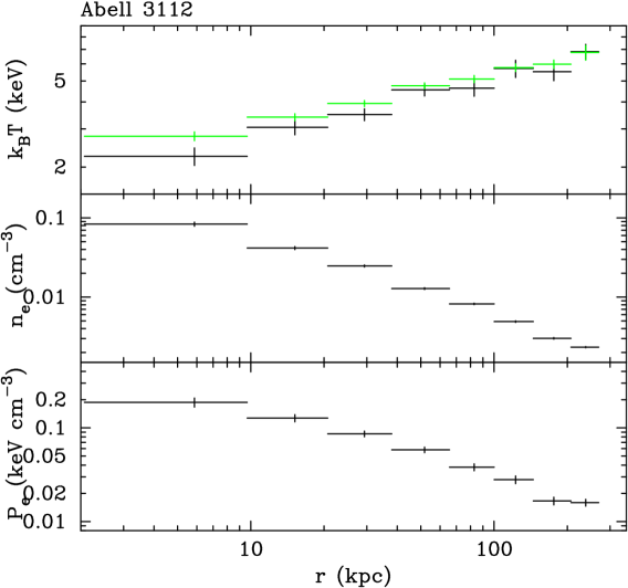
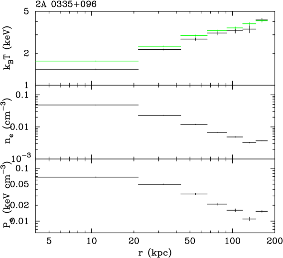
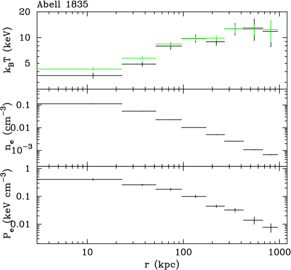
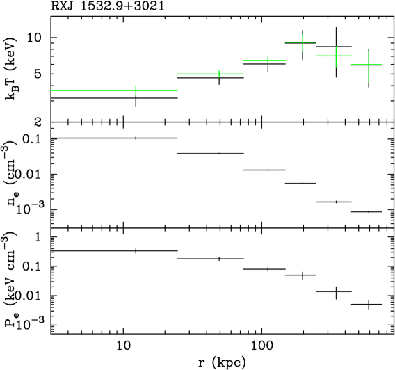
Gas temperature, density and pressure profiles are shown for a representative sample of clusters in Fig 1.

Figure 1: Deprojected gas temperature, density and pressure profiles for a representative sample of clusters. Projected gas temperature profiles are shown in green.

4.1 Temperature and density

The temperature distribution is obtained directly from the spectral fits and the density profile from the normalization of the mekal spectrum, $K=EI/(4\times 10^{14}\pi D_{\rm A}^{2}(1+z)^{2})$, where $EI(=\int n_{\rm e}n_{\rm H}\mathrm{d}V)$ is the emission integral. The electron number density at the centre of each shell is estimated as $\left<n_{\rm e}\right>=(1.2EI/V)^{1/2}$, where we have used the relation $n_{\rm e}\approx 1.2n_{\rm H}$ and $V$ is the volume of the shell.

4.2 Pressure

At the high temperatures and low densities in the ICM the appropriate pressure equation of state is the ideal gas law, given by $P=nk_{\rm B}T$, where $n\approx 1.92n_{\rm e}$ is the number of particles per unit volume. The electron pressure, $P_{\rm e}$, at the midpoint of each shell is computed by multiplying the electron density by the temperature. The uncertainties in $n_{\rm e}$ and $T$ are added in quadrature to find the uncertainty in $P_{\rm e}$ (i.e. the density and temperature are assumed to be independent. We note that contour plots of shell normalization against temperature are approximately circular, showing the assumption is a reasonable one).

5 Mass measurements

5.1 Total mass

Determining masses using X-ray data allows the cluster mass to be computed as a function of radius. The gas is assumed to be in hydrostatic equilibrium within the cluster potential. The equation of hydrostatic equilibrium for a spherically symmetric system is given by

$$M_{\rm tot}(<r_{j})=-\frac{1}{G}\frac{r_{j}^{2}}{\rho_{{\rm gas},j}}\left(\frac{dP}{dr}\right)_{j},$$ (1)

where $P$ is the thermal pressure.

5.1.1 Calculation

The total mass enclosed within radius $r_{j}$ is calculated from Equation 1, where $r_{j}$ is the radial distance from the centre of the cluster to the midpoint between two consecutive shells. The pressure gradient at the midpoint is estimated as

$$\left(\frac{dP}{dr}\right)_{j}=\frac{P_{i+1}-P_{i}}{r_{i+1}-r_{i}},$$ (2)

where $P_{i}$ is the pressure at the centre of the $i$th shell, $r_{i}$ is the radial distance to the centre of the $i$th shell and $r_{j}=(r_{i}+r_{i+1})/2$. The gas density at $r_{j}$ is calculated using linear interpolation, such that

$$\rho_{\rm gas}(r_{j})=\frac{\rho_{\rm gas}(r_{i+1})+\rho_{\rm gas}(r_{i})}{2},$$ (3)

where $\rho_{{\rm gas},i}$, the gas density at the centre of the $i$th shell, is found from the electron number density using the relation $\rho_{{\rm gas},i}=\mu m_{\rm H}n_{{\rm gas},i}\approx 1.92\mu m_{\rm H}n_{{\rm e},i}$. The uncertainties are calculated using a Monte Carlo technique whereby both the pressure and density data are perturbed 1000 times. PKS 0745$-$191 does not exhibit a smooth pressure profile in the centre and so measurements made using Equation 2 do not produce a monotonically increasing mass profile. We compute the mass profile in the inner region of this object by binning together the first and second and the third and fourth data points in the pressure and gas density profiles.

Computing the mass profile involves determining the pressure gradient at the midpoint between the centres of consecutive shells. By estimating the gradient using Equation 2 we effectively fit a straight line between adjacent data points. (The accuracy of the method may therefore be improved by increasing the number of data points). Neighbouring mass points may be slightly correlated, but data points further away than one will not be correlated with one another. Several authors fit a parametric model to the temperature and gas density profiles and use this to compute the mass profile. The data points in this case are not independent and finding the best-fit model to the mass profile using chi-square statistics will be statistically invalid. The method used here, made possible due to the high spatial resolution of the Chandra observatory, therefore provides an improvement over previous analyses.

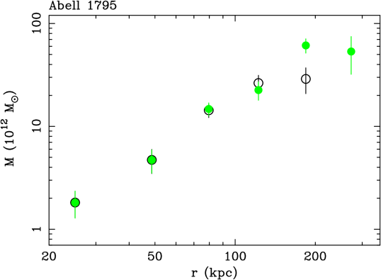
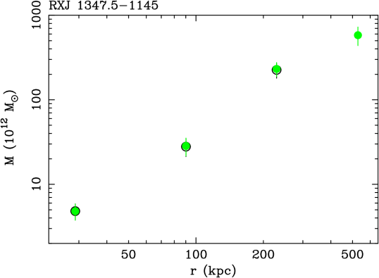
The mass profiles are shown for the sample in Fig. 2. The outer mass data point is removed in all but three clusters (RXJ 1347.5$-$1145, RXJ 1532.9$+$3021 and MS 2137.3$-$2353). This is because the artificially high gas density and pressure in the outer bin causes the outer mass data point to be significantly underestimated in the majority of objects. For the high redshift systems ($z\gtrsim 0.3$) the outer mass data point is estimated to be accurate to within a few per cent. The accuracy of the outer data point is assessed by calculating the mass profile from the data obtained both with and without the outer shell included in the spectral analysis. As an example, the mass profiles obtained for Abell 1795 and RXJ 1347.5$-$1145 are shown in Fig. 3. The percentage decrease in the mass measured in the penultimate shell is less than 1 per cent for RXJ 1347.5$-$1145 and about 50 per cent for Abell 1795 when the outer annulus is not included in the spectral fit.

Removing the outer mass data point in clusters such as Abell 1795 before analysing the mass profile is vital. Current structure formation models predict that the mass profile should ‘turn-over’ at some characteristic radius. If an erroneously low mass data point is included in the outer region then this will wrongly indicate that the profile is curving away from a power-law.

5.1.2 Lensing masses

Mass measurements from strong lensing analyses are also plotted in Fig. 2 for PKS 0745$-$191, RXJ 1347.4$-$1145, Abell 1835 and MS 2137.3$-$2353 (Allen, 1998). In each case the lensing mass is larger than the X-ray mass by a factor of between  1.5$-$3. This discrepancy is also found by Allen (1998) if a single phase spectral model (i.e. no cooling flow) is adopted. It is difficult at this stage to draw any strong conclusions about the difference in the measurements. The lensing results are quoted without uncertainties and there are several difficulties with this method, such as adopting the correct geometry, obtaining accurate arc redshifts and the unknown presence of secondary matter along the line of sight (Wambsganss et al., 2005). Similarly, the masses obtained from the X-ray analysis are also dependent on several assumptions, including the spectral and geometrical models adopted. It will be important in future work to improve on both methods until an agreement is reached.

5.2 Gas mass and gas mass fraction

The integrated gas mass profile is calculated using the sum

$$M_{\rm gas}(<r_{k})=\sum_{i=1}^{n}\frac{4}{3}\pi(r_{k}^{3}-r_{k-1}^{3})\rho_{\rm gas}(r_{i}),$$ (4)

where $r_{k}$ is the radial distance to the outer boundary of the $i$th shell.

The gas mass fraction is the ratio of the total gas mass to the total gravitating mass within a fixed volume

$$f_{\rm gas}=\frac{M_{\rm gas}(<r_{j})}{M_{\rm tot}(<r_{j})}$$ (5)

The total gas mass within $r_{j}$ is computed from the gas mass profiles using linear interpolation. The gas mass fraction profiles are plotted in Fig. 2.

We note that the total integrated mass within a particular volume, calculated from the equation of hydrostatic equilibrium, is dependent upon the pressure gradient and gas density at that radius only, and is completely unaffected by the regions interior (or exterior) to that radius. For the gas mass profile, on the other hand, the integrated mass is calculated by summing from the centre outwards and any error in the measurement at small radii will propagate out to larger radii. However, the gas mass at small radii is much less than at large radii and any uncertainty in the measurements in the core are unlikely to have a significant effect on the gas mass profile further out.

Figure 2: Total (dark plus baryonic) mass profiles (upper) and gas mass fraction profiles (lower). The error bars show the 1 sigma uncertainties in the measurements. The solid line shows the best-fit M${{}_{2}F_{1}}$ model to the data, with $\alpha$ a free parameter in the fit. The dashed line shows the best-fit NFW model ($\alpha=1$) to the data. For the latter model the inner 30 kpc is removed from the fit to the profiles of 2A 0335$+$096, Abell 478, PKS 0745$-$191 and Sersic 159$-$03 (see text). The best-fit scale radius and 1 sigma limits, obtained with $\alpha=1$, are shown by solid and dotted vertical lines respectively. The arrow indicates the best-fit scale radius for the M${{}_{2}F_{1}}$ model. (In the cases where an arrow is not shown the best-fit model tends to a power-law). Lensing masses taken from Allen (1998) are indicated (green filled squares).

Figure 3: Mass profiles computed using data from spectral fits obtained with (green filled circles) and without (black open circles) the outer shell included.

6 Dark matter profiles from simulations

The generalized equation for the density distribution in dark matter halos, including all models with a ‘cuspy’ core, is given by

$$\rho(x)=\frac{\rho_{0}}{x^{\alpha}\left(1+x^{\gamma}\right)^{(\beta-\alpha)/\gamma}},$$ (6)

where $x=r/r_{\rm s}$. The scale radius, $r_{\rm s}$, is a free parameter. The indices ($\alpha$,$\beta$,$\gamma$) for the NFW and M99 models are (1.0,3.0,1.0) and (1.5,3.0,1.5), respectively. A simple analytic model for the mass is easily obtained for each of these special cases, with

$$M(<x)=\begin{cases}4\pi\rho_{0}r_{\rm s}^{3}\left[\mathrm{ln}(1+x)-\frac{x}{1+x}\right]&\text{for NFW}\\ \frac{8}{3}\pi\rho_{0}r_{\rm s}^{3}\mathrm{ln}(1+x^{3/2})&\text{for M99}\end{cases}$$ (7)

A generalized mass profile, valid for any values of the indices, may be written

$$M(<x)=4\pi\rho_{0}r_{\rm s}^{3}\frac{x^{\alpha_{3}}{{}_{2}F_{1}}(\alpha_{3}/\gamma,(\beta-\alpha)/\gamma;(\alpha_{3}+\gamma)/\gamma;-x^{\gamma})}{\alpha_{3}},$$ (8)

where $\alpha_{3}=3-\alpha$. The hypergeometric function ${{}_{2}F_{1}}$ may be evaluated numerically. We refer to this model as M${{}_{2}F_{1}}$.

6.1 Definition of concentration

The mass enclosed within a region $r_{\rm\Delta}$ may be written in terms of the critical density of the Universe,

$$\rho_{\rm crit}(z_{\rm f})=3H(z_{\rm f})^{2}/8\pi G,$$ (9)

where $z_{\rm f}$ is the cluster formation redshift, assumed equal to the observed redshift, such that

$$M_{\Delta}=\frac{4}{3}\pi r_{\Delta}^{3}\rho_{\rm crit}\Delta,$$ (10)

where $\Delta$ is the density contrast. The Hubble parameter, $H(z)=100hE(z)\hbox{$\hbox{${\rm\thinspace km}{\rm\thinspace s^{-1}}\,$}{\rm\thinspace Mpc}^{-1}\,$}$, is derived from the Friedmann equation. In a flat Universe $E(z)^{2}=\Omega_{\rm m}(1+z)^{3}+\Omega_{\Lambda}$.

The concentration, $c_{\Delta}$, is defined such that $c_{\Delta}=r_{\Delta}/r_{\rm s}$. Using this definition the normalization of the density profiles, $\rho_{0}$, may be written as the product of the critical density and a dimensionless parameter, $\delta_{c}$. Substituting $x_{\Delta}=r_{\Delta}/r_{\rm s}=c_{\Delta}$ into the mass formulae above (Equations 7 and  8) at $r=r_{\Delta}$ and setting them equal to Equation 10 yields the following expressions for $\delta_{c}$

$$\delta_{c}=\begin{cases}\frac{\Delta}{3}\frac{c_{\Delta}^{3}}{\mathrm{ln}(1+c_{\Delta})-c_{\Delta}/(1+c_{\Delta})}&\text{for NFW}\\ \frac{\Delta}{2}\frac{c_{\Delta}^{3}}{\mathrm{ln}(1+c_{\Delta}^{3/2})}&\text{for M99}\\ \frac{\Delta}{3}\frac{c_{\Delta}^{\alpha}\alpha_{3}}{{{}_{2}F_{1}}(\alpha_{3}/\gamma,(\beta-\alpha)/\gamma;(\alpha_{3}+\gamma)/\gamma;-c_{\Delta}^{\gamma})}&\text{for M${{}_{2}F_{1}}$}\end{cases}$$ (11)

6.2 Definition of the virial radius

The virial radius separates the region where the cluster is in hydrostatic equilibrium from where matter is still infalling. For $\Omega_{\rm m}+\Omega_{\rm\Lambda}=1$, $r_{\Delta}=r_{\rm vir}$ if $\Delta=\Delta_{\rm vir}=178\Omega_{\rm m}^{0.45}$ (Lacey & Cole, 1993; Eke et al., 1996, 1998). For $\Omega_{\rm m}$ = 0.3, $\Delta_{\rm vir}=104$. In an Einstein-de Sitter Universe, $\Omega_{\rm m}$ = 1.0 and $\Delta_{\rm vir}=178$. A density contrast of $\Delta$ = 200 (or $\Delta$ = 178) is still often used in the literature and $r_{\rm vir}$ and $r_{200}$ (or $r_{178}$) written interchangeably. For purposes of comparison with other work in the literature we adopt $\Delta=200$.

7 Modelling the observed mass profiles

CDM simulations make two robust predictions concerning the distribution of mass in dark matter halos: the shape of the mass profile differs strongly from a power-law, and the power-law slope of the inner density profile lies in the range $1.0\lesssim\alpha\lesssim 1.5$ (see, for example, Navarro et al., 2004). These properties are investigated for the observed mass profiles below.

7.1 General shape of the mass profile

The mass profiles in Fig. 2 are fit with the generalized mass model in Equation 8, with $\beta$ and $\gamma$ fixed at 1.0. Fig. 4 shows the variation in concentration parameter, scale radius, virial radius ($r_{200}$) and chi-square with inner slope as $\alpha$ is stepped through values between 0.0 and 2.0 and the fit is minimized with respect to $c$ and $r_{\rm s}$. (Note that the scale radius and concentration are highly negatively correlated). The virial radius is computed by substituting $c_{\Delta}=r_{\Delta}/r_{\rm s}$ into Equation 11.

Figure 4: Plots showing variation in concentration, scale radius, virial radius and $\Delta\chi^{2}$ ($=\chi^{2}-\chi^{2}_{\rm{min}}$, where $\chi^{2}_{\rm{min}}$ is the minimum chi-square) for values of the inner slope $\alpha$ between 0 and 2. The dotted horizontal lines in the bottom panel show the 1$\sigma$ (68.3 per cent), 2$\sigma$ (95.4 per cent) and 3$\sigma$ (99.7 per cent) confidence levels for alpha. The grey shaded regions show the parameter values which lie within the one-sigma confidence interval. Note that when the concentration drops below 1.0 the scale radius is larger than the virial radius and the profile tends to a power-law. Fit parameters determined with the inner 30 kpc excluded are shown with dashed lines, and the one-sigma confidence limits shown by green dashed lines. (If only one green dashed line is shown then the lower limit on alpha is less than zero).

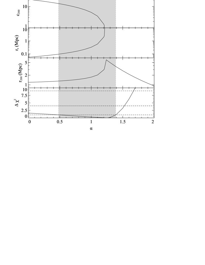
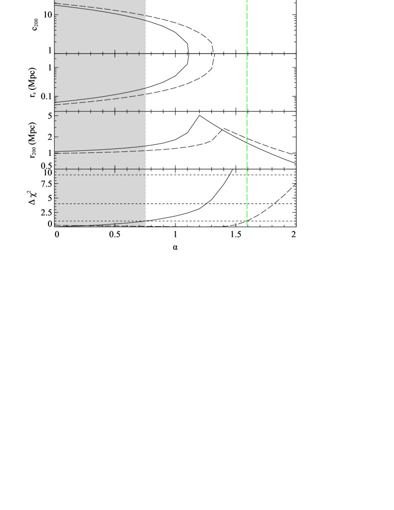
If the best-fit concentration is less than 1.0 for a particular value of $\alpha$, then the mass model does not agree with CDM predictions i.e. the characteristic radius, $r_{\rm s}$, at which the profile ‘turns-over’ is greater than the virial radius. In Table 3 we show the best-fit parameters for the $M_{2}F_{1}$ and power-law ($M_{\rm pow}\propto r^{3-\alpha}$) models. When the best-fit concentration for the $M_{2}F_{1}$ model is $c\ll 1.0$ the model tends to a power-law. We refer to the best-fit model as a power-law when the best-fit concentration is less then 1.0. Although not strictly true, the description serves as a useful distinction between profiles which are consistent ($c>1$) and those which are inconsistent ($c<1$) with CDM model predictions.

Cluster	M${{}_{2}F_{1}}$ model					Power-law model
	$\alpha$	$c_{200}$	$r_{\rm s}$	$r_{200}$	$\chi^{2}$(dof)	$\alpha$	$\chi^{2}$(dof)
			(Mpc)	(Mpc)
Abell 3112	1.31${}^{+0.15}_{-0.55}$	–	–	4.6	0.8(3)	1.31${}^{+0.15}_{-0.16}$	0.8(4)
2A 0335$+$096	0.00${}^{+0.15}_{-0.00}$	12	0.14	1.7	6.5(2)	0.55${}^{+0.09}_{-0.09}$	12.3(3)
	0.00${}^{+1.21}_{-0.00}$	15	0.08	1.2	2.3(1)	1.05${}^{+0.21}_{-0.19}$	0.7(2)
Abell 478	0.49${}^{+0.45}_{-0.49}$	9.0	0.22	2.0	6.7(5)	0.94${}^{+0.10}_{-0.10}$	7.8(6)
	1.14${}^{+0.15}_{-0.63}$	–	–	9.2	5.4(4)	1.14${}^{+0.15}_{-0.16}$	5.4(5)
PKS 0745$-$191	0.00${}^{+0.41}_{-0.00}$	14	0.13	1.8	2.5(2)	0.91${}^{+0.15}_{-0.16}$	6.1(3)
	0.00${}^{+1.49}_{-0.00}$	18	0.09	1.6	0.4(1)	1.32${}^{+0.22}_{-0.22}$	0.9(2)
RXJ 1347.5$-$1145	1.10${}^{+0.27}_{-0.41}$	3.2	0.90	2.9	3.0(1)	1.30${}^{+0.10}_{-0.10}$	3.4(2)
Abell 1795	1.24${}^{+0.15}_{-0.56}$	–	–	5.8	2.6(2)	1.24${}^{+0.15}_{-0.16}$	2.6(3)
Abell 1835	0.52${}^{+0.53}_{-0.52}$	9.2	0.20	1.8	5.9(3)	1.14${}^{+0.11}_{-0.11}$	7.5(4)
Abell 3581	0.88${}^{+0.65}_{-0.88}$	12	0.05	0.7	1.3(3)	1.34${}^{+0.22}_{-0.24}$	1.5(4)
Abell 2029	0.74${}^{+0.34}_{-0.61}$	8.9	0.21	1.9	2.4(4)	1.13${}^{+0.09}_{-0.09}$	4.1(5)
RXJ 1532.9$+$3021	0.85${}^{+0.49}_{-0.85}$	4.3	0.46	2.0	1.2(2)	1.18${}^{+0.20}_{-0.19}$	1.6(3)
MS 2137.3$-$2352	1.25${}^{+0.14}_{-0.77}$	–	–	5.9	0.2(1)	1.25${}^{+0.14}_{-0.15}$	0.2(2)
Sersic 159$-$03	0.00${}^{+0.75}_{-0.00}$	17	0.06	1.1	3.4(3)	1.09${}^{+0.14}_{-0.15}$	6.0(4)
	1.20${}^{+0.39}_{-1.20}$	3.4	0.42	1.4	2.5(2)	1.38${}^{+0.21}_{-0.21}$	2.5(3)

Table 3: Best-fit slope $\alpha$ and corresponding chi-square for the M${{}_{2}F_{1}}$ and power-law models. The second row for 2A 0335$+$096, Abell 478, PKS 0745$-$191 and Sersic 159$-$03 shows the best-fit with the inner 30 kpc excluded. The best-fit concentration, scale radius and virial radius are shown for the M${{}_{2}F_{1}}$ model. The concentration and scale radius are not shown for clusters where the best-fit tends to a power-law (i.e. $c<<1.0$).

With $\alpha$ a free parameter in the fits, the concentration is consistent with both $c>1$ and $c<1$ within the one sigma uncertainties for half the objects analysed (Abell 3112, RXJ 1347.5$-$1145, Abell 1795, Abell 3581, RXJ 1532.9$+$3021 and MS 2137.3$-$2353; see shaded regions in Fig. 4). In four clusters (2A 0335$+$096, Abell 478, PKS 0745$-$191 and Sersic 159$-$03) the best-fit concentration is greater than 1.0 at the 68 per cent confidence level; although the best-fit inner slope in these objects is shallower than predicted by CDM simulations. Abell 1835 and Abell 2029 are the only two objects for which a power-law is ruled out at the 1$\sigma$ level and the inner slope is consistent with the CDM model.

7.2 Inner slope measurements

The best-fit inner slope and 1$\sigma$ uncertainties are plotted for each object in Fig. 5. Also shown are the 3$\sigma$ upper limits on the slope. Clusters with a best-fit concentration less than 1.0 are indicated. It is clear from the plot that 8 out of the 12 clusters analysed are consistent with the CDM model. Furthermore, the points appear to scatter around $\alpha=1.0$, rather than $\alpha=1.5$. An inner logarithmic slope of $\alpha=2$ is ruled out at the 3$\sigma$ level in all objects except Abell 3581; the mass profiles would therefore seem to rule out the single isothermal sphere (SIS) model which has been widely used in the literature (e.g. Binney & Tremaine, 1987). We note that there is no obvious correlation between the cluster mass and the best-fit inner slope, although the uncertainties are too large to justify any correlation tests on the data.

Figure 5: Left: best-fit inner slope. Right: best-fit inner slope with inner 30 kpc removed in 2A 0335$+$096, Abell 478, PKS 0745$-$191 and Sersic 159$-$03. The error bars show the 1 sigma uncertainties and the downward arrows the 3 sigma upper limits. An open circle is used to indicate clusters with a best-fit concentration less than 1.0. The clusters are plotted from left to right in the same order as they are listed (from top to bottom) in Table 1.

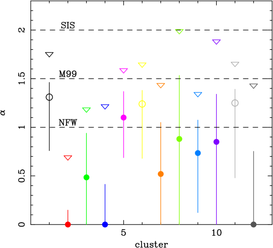
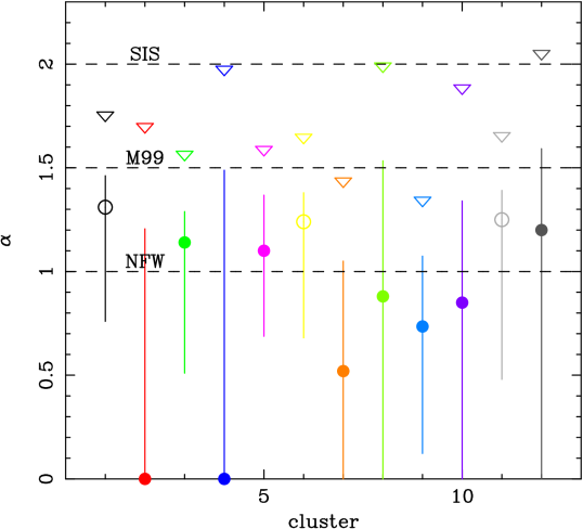
The four clusters which are inconsistent with an inner slope of 1.0 at the 1$\sigma$ level are 2A 0335$+$096, Abell 478, PKS 0745$-$191 and Sersic 159$-$03, with Abell 478, Sersic 159$-$03 and PKS 0745$-$191 consistent with $\alpha=1.0$ at the 2 sigma level. Only 2A 0335$+$096 disagrees with CDM predictions with 99.7 per cent confidence. We note that this is also the object for which the spectral model used provides the poorest fit (see Section 3.5) and, as discussed below, the temperature distribution in the centre is highly asymmetric between the northern and southern sectors of the cluster. The presence of an asymmetric temperature distribution in 2A 0335$+$096 has been shown previously by Mazzotta et al. (2003).

In a recent study, Katayama & Hayashida (2004) find that six out of the twenty clusters in their sample (including Abell 478, PKS 0745$-$191 and 2A 0335$+$096) have a slope lower than unity at the 90 per cent confidence level. The authors interpret this result as being in agreement with the ‘flat core problem’ found in observations of low mass objects.

The method used for computing the mass profiles relies on the assumptions of hydrostatic equilibrium and spherical symmetry. Whether or not the former condition is met is difficult to ascertain. Katayama & Hayashida (2004) touch on this problem by highlighting objects which exhibit obvious structure in their cores, suggesting that this may indicate a break from hydrostatic equilibrium, as well as the possibility of affecting the ambient temperature and density profile measurements. They conclude that some objects have flat inner slopes (Abell 478, PKS 0745$-$191, ZW 3146), even when those with central structure (2A 0335$+$096 and Abell 2597) are removed.

In Fig 5 we plot the best-fit inner density slopes when the inner $\sim 30\rm\thinspace kpc$ is removed from the fits to 2A 0335$+$096, Abell 478, PKS 0745$-$191 and Sersic 159$-$03. It is clear that it is the innermost data point in each of these clusters which is forcing the best-fit to be flat. The question is ‘how far can we trust data from the central 30 kpc?’. The challenge will be to determine the extent of any non-thermal pressure support in the central regions of these objects.

7.3 Symmetry of the temperature distribution

One clue that the gas is disturbed and not in hydrostatic equilibrium may be suggested by asymmetries in the temperature distribution. Here we investigate whether there is any correlation between the degree of symmetry in the temperature distribution and the inner slope of the mass profile.

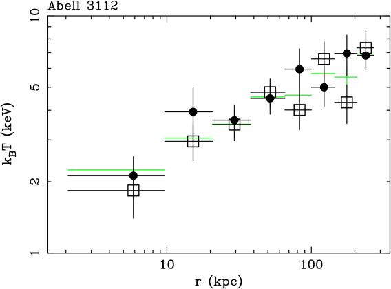
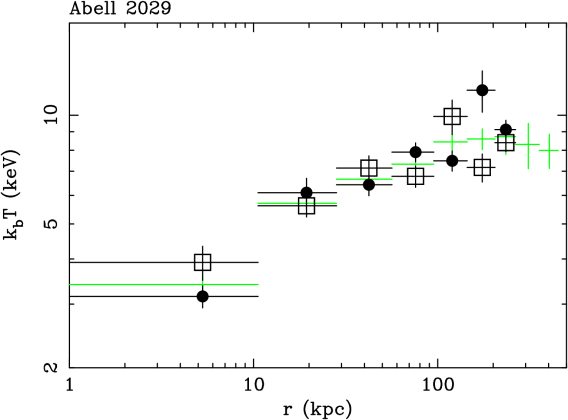
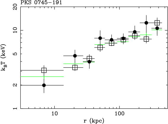
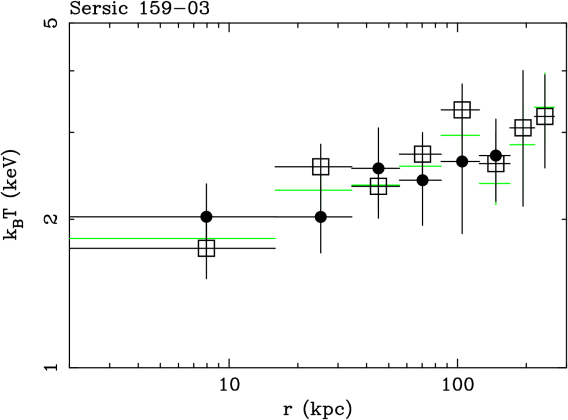
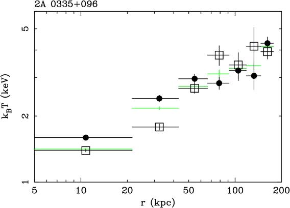
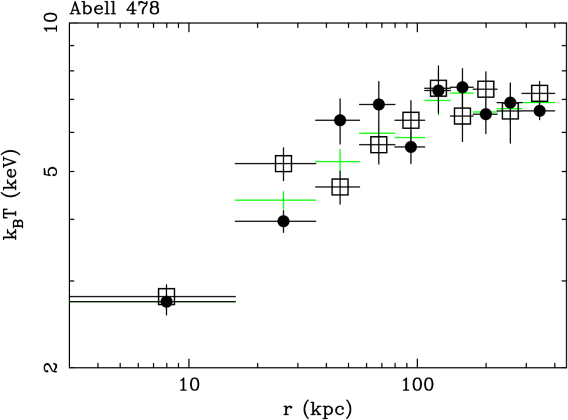
Fig 6 shows the temperature distributions obtained for each of the clusters showing a flat inner density profile, together with two clusters which are consistent with the CDM mass model.

The temperature distribution of 2A 0335$+$096 is clearly asymmetric within the central $\sim$50 kpc. This is unsurprising given that Mazzotta et al. (2003) have shown the central region contains many blobs of gas at different projected temperatures. The asymmetry does not, therefore, necessarily mean that the gas is not in hydrostatic equilibrium, but does suggest that the temperature distribution obtained from the spectral analysis may not be that of the ambient gas. In this case, the central mass measurements obtained may be incorrect. We note that Mazzotta et al. (2003) find a significant asymmetry in the temperature distribution at radii $>100$ kpc. We also find that the southern half of the cluster is hotter than the northern half in the outer region, but the effect is not so pronounced. There are several differences between the analysis carried out here and the one by Mazzotta et al. (2003) which may give rise to a discrepancy in the measured temperature distributions. Firstly, Mazzotta et al. (2003) extract spectra in elliptical rather than circular annuli and are therefore probing different regions of the cluster. If the temperature distribution is not symmetrical then this may lead to significant differences in the temperatures measured. In addition, Mazzotta et al. (2003) plot the projected temperatures and allow the absorption column density to vary between shells.

For the rest of the sample there is little evidence for a correlation between the inner slope and the degree of symmetry in the temperature distribution.

Figure 6: Plots showing the temperature distribution extracted from the northern (filled circles) and southern (open squares) sectors of the cluster. Also shown is the temperature obtained from the whole annulus at each radius (green).

7.4 Observed gas mass fraction profiles

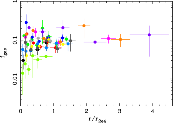
The gas mass fraction profiles are shown in Fig. 2. The profiles were calculated using the relation $f_{\rm gas}(<r)=M_{\rm gas}(<r)/M_{\rm tot}(<r)$, where $M_{\rm tot}$ is the total model-independent mass. The profiles are plotted for the whole sample in Fig 7, with the $x$-axis scaled by $r_{2\times 10^{4}}$ (see Section 7.4). The profiles show a variety of behaviour within $r\sim 0.02r_{\rm vir}$, with an apparent flattening at $f_{\rm gas}\sim 0.1$ outside this region, similar to the results of Allen et al. (2004).

Figure 7: Gas mass fraction profiles for the sample with the $x$-axis scaled by $r_{2\times 10^{4}}$ (see Table 4). The colour-coding is the same as used in Fig 5.

7.4.1 Inner region

A high value of $f_{\rm gas}$, relative to the values outside $r\sim 0.02r_{\rm vir}$, is seen in the central bin of 2A 0335$+$096, Abell 478, PKS 0745$-$191 and Sersic 159$-$03. These are the only objects in the sample for which the best-fit inner slope, $\alpha$, to the mass profile is less than 1.0 (see Fig 5), suggesting a link between a high measured central gas mass fraction and an apparently shallow inner mass density profile. The central rise in $f_{\rm gas}$ is clearly seen in Fig. 8 where we plot scaled gas mass fraction profiles for the three clusters where the $f_{\rm gas}$ peak is most obvious (2A 0335$+$096, Abell 478 and PKS 0745$-$191), together with two low redshift clusters (Abell 3112 and Abell 1795), whose best-fit mass profiles are consistent with $\alpha=1.0$, for comparison. The latter two objects show an increase in $f_{\rm gas}$ from the centre outwards, as expected from CDM simulations (Eke et al., 1998). With the exception of Abell 3581, whose profile drops towards the centre, the remaining objects in the sample have relatively flat $f_{\rm gas}$ profiles in the inner region.

Figure 8: Gas mass fraction profiles for Abell 3112 (black), 2A 0335$+$096 (red), Abell 478 (green), PKS 0745$-$191 (blue) and Abell 1795 (yellow).

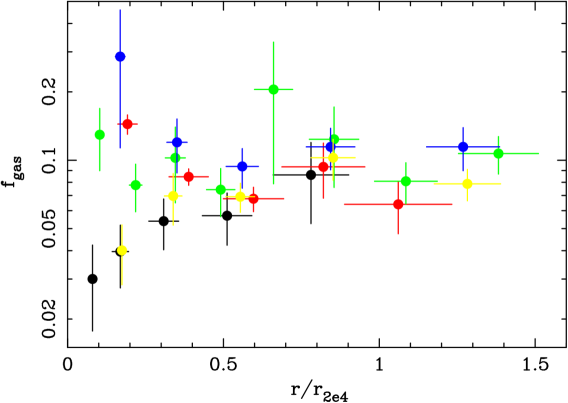
Katayama & Hayashida (2004) find a negative correlation between $\alpha$ and the value of $f_{\rm gas}$ near the centre of the cluster. They interpret this as a tendency for clusters with gas-rich cores to have flat central density profiles. It seems just as likely that the high gas mass fraction measured in the central parts of these objects results from an underestimation of the total mass, supporting the presence of non-thermal pressure in the core or suggesting incorrect spectral modelling of the data (note that the spectral fit to the emission from the centre of 2A 0335$+$096 is poor).

7.5 NFW model fits

The majority of the clusters in the sample are consistent with the NFW mass model i.e. $\alpha=1.0$ (see Fig. 5). Here we find the best-fit scale radius and concentration for each cluster assuming an NFW profile. (For clusters where the NFW model is excluded at the 1 sigma level, we remove the inner 30 kpc from the fit). It is important to stress that attempting to measure $r_{\rm s}$ is pushing the data to its limits since the best-fit scale radius in general lies beyond the radius at which mass measurements can be made (see Fig. 2). The values obtained for $r_{\rm s}$ are therefore strongly dependent on the outermost datapoint in the mass profile. It also makes the value difficult to constrain and, while some of the clusters show evidence for a turn-over in the mass profile, more precise determination of the scale radius would require mass measurements out to a larger fraction of the virial radius.

We compute the concentration at three overdensities: $\Delta=2\times 10^{4}$, 2500 and 200. For $\Delta=2\times 10^{4}$ the value obtained for $r_{\Delta}$ is independent of the accuracy of $r_{\rm s}$ since in each case $r_{\Delta}$ lies within the radius at which mass measurements have been obtained. However, for $\Delta=200$ the value obtained for $r_{200}$ is highly dependent on the accuracy of $r_{\rm s}$ (since it involves extrapolating the NFW model using $r_{\rm s}$). The values for $r_{200}$ are shown for interest, but are not used for any subsequent analysis. The concentration is also computed at $\Delta=2500$. This allows comparison of our results for PKS 0745$-$191, Abell 1835, RXJ 1347.5$-$1145 and MS 2137.3$-$2352 with those found by Allen et al. (2001). (Note that for the more massive clusters $r_{2500}$ lies within the radius at which mass measurements have been obtained). The data used here for PKS 0745$-$191, Abell 1835 and RXJ 1347.5$-$1145 are the same data used by Allen et al. (2001). The values of $r_{2500}$ are consistent between the two studies within the 1 sigma uncertainties. However, Allen et al. (2001) generally find a higher concentration (and therefore lower scale radius) than the results found here. The difference in values is not surprising given the discussion above concerning the difficulty of measuring $r_{\rm s}$.

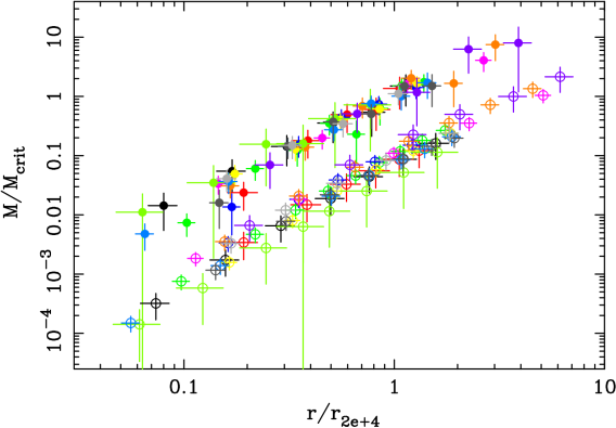
The best-fit parameters are shown in Table 4. The mass enclosed within a density contrast of 2$\times$10⁴ is computed using Equation 10. The cluster mass profiles, with the $x$-axis scaled by $r_{\Delta}$, are shown in Fig. 9. The $y$-axis for each mass profile is scaled by $M_{\rm crit}=(4/3)\pi r_{\Delta}^{3}\rho_{\rm crit}\Delta$. Each mass profile should therefore coincide if the concentration varies little from halo to halo.

Figure 9: Scaled mass profiles: total (filled circles) and gas (open circles) mass profiles. The colour-coding is the same as used in Fig 5.

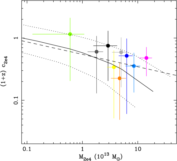
$N$-body simulations predict a weak dependence of halo concentration on mass, with $c_{\rm vir}\propto M_{\rm vir}^{-a}$ and $a\sim 0.1$ for all halos at a given redshift. In Fig. 10 we plot $c_{2\times 10^{4}}$ against $M_{2\times 10^{4}}$. (Note that we do not plot $c_{200}$ against $M_{200}$ here since the calculation of $M_{200}$ depends on $r_{200}$ which is itself an uncertain number). The concentration is scaled to a redshift of zero using the concentration–redshift dependence found in $N$-body simulations by Bullock et al. (2001). The relation predicts that for haloes of the same mass the concentration is proportional to $(1+z)^{-1}$. We show the best-fit power-law model to the data along with the theoretical prediction of Bullock et al. (2001). The theoretical model is applicable out to halo masses of $M_{\rm vir}\lesssim 10^{16}M_{\odot}$, giving rise to a cut-off in the predicted $c_{2\times 10^{4}}$–$M_{2\times 10^{4}}$ relation at $M_{2\times 10^{4}}\sim 10^{14}M_{\odot}$. The best-fit power-law index is $a\sim 0.2$. The data appear to agree well with the theoretical model of Bullock et al. (2001).

Figure 10: Plot showing the dependence of concentration on halo mass. The theoretical mass–concentration relation predicted by Bullock et al. (2001) (solid curve) and one-sigma confidence limits (dotted curves). Also shown is the best-fit power-law model to the data (dashed line). The colour-coding is the same as used in Fig 5.

Cluster	$r_{\rm s}$	$c_{200}$	$r_{200}$	$c_{2\times 10^{4}}$	$r_{2\times 10^{4}}$	$M_{2\times 10^{4}}$	$r_{2500}$	$\chi^{2}$(dof)
	(Mpc)		(Mpc)		(Mpc)	($10^{13}$ M⊙)	(Mpc)
Abell 3112	0.19${}^{+0.39}_{-0.09}$	7.06${}^{+3.62}_{-3.23}$	1.32${}^{+0.88}_{-0.35}$	0.70${}^{+0.57}_{-0.44}$	0.13${}^{+0.02}_{-0.02}$	2.9${}^{+1.5}_{-1.1}$	0.42${}^{+0.19}_{-0.09}$	1.3(4 )
2A 0335$+$096	0.13${}^{+5.38}_{-0.10}$	8.18${}^{+18.83}_{-7.20}$	1.05${}^{+4.42}_{-0.39}$	0.88${}^{+3.22}_{-0.85}$	0.11${}^{+0.02}_{-0.01}$	1.7${}^{+1.0}_{-0.5}$	0.34${}^{+0.56}_{-0.10}$	1.7(1)
Abell 478	1.03${}^{+\to\infty}_{-0.63}$	2.88${}^{+2.02}_{-\to 2.88}$	2.97${}^{+14.8}_{-1.02}$	0.16${}^{+0.24}_{-\to 0.16}$	0.16${}^{+0.02}_{-0.01}$	5.7${}^{+1.7}_{-1.5}$	0.76${}^{+0.67}_{-0.19}$	5.6(5)
PKS 0745$-$191	0.36${}^{+0.98}_{-0.20}$	5.46${}^{+3.22}_{-2.88}$	1.96${}^{+1.51}_{-0.50}$	0.47${}^{+0.48}_{-0.34}$	0.17${}^{+0.02}_{-0.01}$	6.3${}^{+1.9}_{-1.6}$	0.59${}^{+0.27}_{-0.11}$	0.6(2 )
RXJ 1347.5$-$1145	0.60${}^{+0.46}_{-0.22}$	4.37${}^{+1.39}_{-1.24}$	2.64${}^{+0.70}_{-0.48}$	0.33${}^{+0.18}_{-0.14}$	0.20${}^{+0.02}_{-0.02}$	14.3${}^{+3.6}_{-3.7}$	0.76${}^{+0.13}_{-0.10}$	3.0(2)
Abell 1795	0.45${}^{+1.59}_{-0.23}$	4.28${}^{+2.23}_{-2.41}$	1.94${}^{+1.86}_{-0.51}$	0.32${}^{+0.30}_{-0.24}$	0.14${}^{+0.01}_{-0.01}$	3.7${}^{+1.0}_{-0.8}$	0.55${}^{+0.28}_{-0.11}$	3.0(3)
Abell 1835	0.80${}^{+1.59}_{-0.38}$	3.13${}^{+1.37}_{-1.44}$	2.50${}^{+1.55}_{-0.64}$	0.18${}^{+0.16}_{-0.12}$	0.15${}^{+0.01}_{-0.01}$	4.7${}^{+1.4}_{-1.4}$	0.65${}^{+0.20}_{-0.12}$	6.6(4)
Abell 3581	0.07${}^{+0.23}_{-0.04}$	9.81${}^{+6.30}_{-5.40}$	0.69${}^{+0.65}_{-0.20}$	1.13${}^{+1.05}_{-0.79}$	0.08${}^{+0.02}_{-0.01}$	0.6${}^{+0.6}_{-0.3}$	0.23${}^{+0.16}_{-0.06}$	1.3(4)
Abell 2029	0.58${}^{+0.94}_{-0.25}$	4.38${}^{+1.64}_{-1.76}$	2.52${}^{+1.45}_{-0.59}$	0.33${}^{+0.22}_{-0.19}$	0.19${}^{+0.02}_{-0.02}$	8.5${}^{+2.7}_{-2.3}$	0.72${}^{+0.26}_{-0.13}$	2.9(5)
RXJ 1532.9$+$3021	0.81${}^{+13.07}_{-0.53}$	2.77${}^{+2.28}_{-2.28}$	2.24${}^{+4.72}_{-0.85}$	0.15${}^{+0.27}_{-0.14}$	0.12${}^{+0.02}_{-0.02}$	2.9${}^{+1.3}_{-1.3}$	0.56${}^{+0.31}_{-0.15}$	1.3(3)
MS 2137.3$-$2353	0.34${}^{+0.74}_{-0.16}$	5.28${}^{+2.41}_{-2.52}$	1.74${}^{+1.22}_{-0.42}$	0.45${}^{+0.35}_{-0.30}$	0.15${}^{+0.02}_{-0.01}$	5.0${}^{+1.7}_{-1.4}$	0.52${}^{+0.22}_{-0.10}$	0.4(2)
Sersic 159$-$03	0.20${}^{+0.37}_{-0.10}$	6.16${}^{+3.42}_{-2.79}$	1.22${}^{+0.70}_{-0.30}$	0.57${}^{+0.52}_{-0.36}$	0.11${}^{+0.01}_{-0.01}$	1.8${}^{+0.6}_{-0.5}$	0.38${}^{+0.14}_{-0.07}$	2.5(3)

Table 4: Best-fit NFW model parameters for $\Delta=200$ and $\Delta=2\times 10^{4}$. Also shown are the scaled radii enclosing a density contrast of $\Delta=2500$.

8 Summary

The shape of the mass distribution in virialized halos provides a sensitive test of the CDM paradigm. In this paper we have analysed the mass profiles of a sample of galaxy clusters. The main results are as follows:

• The mass distribution in the majority of the objects studied are consistent with the NFW model (Navarro et al., 1995). Four objects in the sample (2A 0335$+$096, Abell 478, PKS 0745$-$191 and Sersic 159$-$03) exhibit a flatter core.

• The gas mass fraction measured in the central region of the clusters with flat core density profiles is high, indicating that the total mass may be underestimated within the central $\sim 30\rm\thinspace kpc$ of these objects. If this is the case, then either a significant non-thermal pressure component exists in the core, or the X-ray emission has been incorrectly modelled. For 2A 0335$+$096 the central temperature distribution is asymmetric, suggesting that the temperature and density obtained may not accurately represent the ambient gas properties in the core for this object.

• CDM simulations predict that the mass distribution in virialized halos differs from a power-law, turning-over at a characteristic radius, $r_{\rm s}=r_{\rm vir}/c$.

  • With $\alpha$ a free parameter in the fits, a power-law density profile is ruled out at the 1 sigma level in Abell 1835 and Abell 2029. (A power-law is also ruled out at the 1 sigma level in 2A 0335+096, Abell 478, PKS 0745$-$191 and Sersic 159$-$03, although the inner slope in these objects is inconsistent with CDM predictions). Otherwise, we find no strong evidence for the expected turn-over in the mass profile. For three objects in the sample (Abell 3112, Abell 1795 and MS 2137.3$-$2353) the best-fit model is a power-law.

  • With $\alpha$ fixed at 1.0 the best-fit model is inconsistent with a power-law model for all objects except Abell 478.

• The mass–concentration relation at a density contrast of $2\times 10^{4}$ is consistent with the theoretical prediction from $N$-body simulations by Bullock et al. (2001).

9 Discussion

In the CDM scenario, simulations predict a universal form for the distribution of dark matter in virialized halos, independent of both mass and cosmological parameters (Navarro et al., 1995, 1996, 1997). The universal density profile has a cuspy core, $\rho\propto r^{-\alpha}$, rolling over to $\rho\propto r^{-3}$ at a characteristic radius known as the scale radius. The majority of the mass profiles obtained for the cluster sample in this paper are consistent with the NFW model; only four objects exhibit shallower density cores (2A 0335$+$096, Abell 478, PKS 0745$-$191 and Sersic 159$-$03). The discrepancy between the mass distribution measured in these systems and the NFW profile need not indicate any problem with the CDM paradigm, but may instead result from an underestimation of the core mass. The high gas mass fraction measured in the central region of all four systems with flat inner density profiles certainly suggests that this may be the case. Spuriously low mass measurements could be caused by the presence of non-thermal pressure support in the inner regions of these objects and/or incorrect spectral modelling of the emission from clusters with significant core substructure. Another possibility concerns the importance of non-spherical effects on the measured mass distribution. Hayashi et al. (2004) have recently shown that rotation curves obtained from galaxies with triaxial halos may, in some cases, infer an erroneously flat core to the mass profile if spherical symmetry is assumed. The effects of non-axial symmetry on X-ray measurements of cluster masses have been investigated by Piffaretti et al. (2003). The authors show that the core mass will be underestimated if the halo is compressed along the line-of-sight. It is interesting that both Abell 478 and PKS 0745$-$191 both appear highly elliptical. Analytic solutions to the hydrostatic equation for gas residing in a triaxial dark matter potential have been computed for isothermal and polytropic temperature distributions by Lee & Suto (2003). These formula may in future work be applied to clusters to compute the mass distribution.

Determining whether or not the flat cores measured in some clusters are real is of great importance to cosmological and cluster studies; if they are real, then either our understanding of dark matter is incorrect, or non-gravitational processes, such as dynamical friction acting on cluster galaxies moving through the core (El-Zant et al., 2004), modify the mass distribution.

The work carried out here has put some constraints on the mass distribution in a sample of galaxy clusters. Tighter constraints will be possible by imaging the clusters out to larger radii or, for the case of high redshift objects, by taking longer exposures, so that the radius at which the profile ‘turns-over’ may be robustly detected.

In future work it will be important to investigate effects which might reconcile the observed flat density profiles found in this study with CDM model predictions. One possible cause for the discrepancy is non-thermal pressure support in the core. Sanders et al. (2005) find inverse Compton emission from relativistic electrons which can contribute significant pressure near the centre of the Perseus cluster. Careful comparison of X-ray and lensing masses will also be important.

References

- Allen (1998) Allen S. W., 1998, MNRAS, 296, 392
- Allen et al. (2004) Allen S. W., Schmidt R. W., Ebeling H., Fabian A. C., van Speybroeck L., 2004, MNRAS, 353, 457
- Allen et al. (2001) Allen S. W., Schmidt R. W., Fabian A. C., 2001, MNRAS, 328, L37
- Anders & Grevesse (1989) Anders E., Grevesse N., 1989, GeCoA, 53, 197
- Arabadjis et al. (2004) Arabadjis J. S., Bautz M. W., Arabadjis G., 2004, ApJ, 617, 303
- Arnaud (1996) Arnaud K., 1996, in Astronomical Society of the Pacific conference series, Vol. 101, Jacoby G. H., Barnes J., ed, Astronomical Data Analysis Software and Systems, p. 17
- Bîrzan et al. (2004) Bîrzan L., Rafferty D. A., McNamara B. R., Wise M. W., Nulsen P. E. J., 2004, ApJ, 607, 800
- Balucinska-Church & McCammon (1992) Balucinska-Church M., McCammon D., 1992, ApJ, 400, 699
- Binney & Tremaine (1987) Binney J., Tremaine S., 1987, Galactic dynamics. Princeton University Press, Princeton, NJ
- Bullock et al. (2001) Bullock J. S., Kolatt T. S., Sigad Y., Somerville R. S., Kravtsov A. V., Klypin A. A., Primack J. R., Dekel A., 2001, MNRAS, 321, 559
- Cole & Lacey (1996) Cole S., Lacey C., 1996, MNRAS, 281, 716
- Crone et al. (1994) Crone M. M., Evrard A. E., Richstone D. O., 1994, ApJ, 434, 402
- Dickey & Lockman (1990) Dickey J. M., Lockman F. J., 1990, ARA&A, 28, 215
- Diemand et al. (2005) Diemand J., Zemp M., Moore B., Stadel J., Carollo M., 2005, ArXiv Astrophysics e-prints
- Dubinski & Carlberg (1991) Dubinski J., Carlberg R. G., 1991, ApJ, 378, 496
- Eke et al. (1996) Eke V. R., Cole S., Frenk C. S., 1996, MNRAS, 282, 263
- Eke et al. (1998) Eke V. R., Navarro J. F., Frenk C. S., 1998, ApJ, 503, 569
- El-Zant et al. (2004) El-Zant A. A., Hoffman Y., Primack J., Combes F., Shlosman I., 2004, ApJ, 607, L75
- Fillmore & Goldreich (1984) Fillmore J. A., Goldreich P., 1984, ApJ, 281, 9
- Frenk et al. (1988) Frenk C. S., White S. D. M., Davis M., Efstathiou G., 1988, ApJ, 327, 507
- Fukushige & Makino (1997) Fukushige T., Makino J., 1997, ApJ, 477, L9
- Fukushige & Makino (2001) Fukushige T., Makino J., 2001, ApJ, 557, 533
- Fukushige & Makino (2003) Fukushige T., Makino J., 2003, ApJ, 588, 674
- Ghigna et al. (2000) Ghigna S., Moore B., Governato F., Lake G., Quinn T., Stadel J., 2000, ApJ, 544, 616
- Gunn & Gott (1972) Gunn J. E., Gott J. R. I., 1972, ApJ, 176, 1
- Hayashi et al. (2004) Hayashi E. et al., 2004, ApJ, submitted (astro-ph/0408132)
- Hayashi et al. (2003) Hayashi E. et al., 2003, MNRAS, submitted (astro-ph/0310576)
- Hoffman & Shaham (1985) Hoffman Y., Shaham J., 1985, ApJ, 297, 16
- Jing & Suto (2000) Jing Y. P., Suto Y., 2000, ApJ, 529, L69
- Johnstone et al. (2004) Johnstone R. M., Fabian A. C., Morris R. G., Taylor G. B., 2004, MNRAS, accepted (astro-ph/0410154)
- Katayama & Hayashida (2004) Katayama H., Hayashida K., 2004, Advances in Space Research, 34, 2519
- Klypin et al. (2001) Klypin A., Kravtsov A. V., Bullock J. S., Primack J. R., 2001, ApJ, 554, 903
- Kravtsov et al. (1997) Kravtsov A. V., Klypin A. A., Khokhlov A. M., 1997, ApJS, 111, 73
- Lacey & Cole (1993) Lacey C., Cole S., 1993, MNRAS, 262, 627
- Lee & Suto (2003) Lee J., Suto Y., 2003, ApJ, 585, 151
- Liedahl et al. (1995) Liedahl D. A., Osterheld A. L., Goldstein W. H., 1995, ApJ, 438, L115
- Mazzotta et al. (2003) Mazzotta P., Edge A. C., Markevitch M., 2003, ApJ, 596, 190
- Mewe et al. (1985) Mewe R., Gronenschild E. H. B. M., van den Oord G. H. J., 1985, A&AS, 62, 197
- Moore et al. (1999) Moore B., Quinn T., Governato F., Stadel J., Lake G., 1999, MNRAS, 310, 1147
- Navarro et al. (1995) Navarro J. F., Frenk C. S., White S. D. M., 1995, MNRAS, 275, 720
- Navarro et al. (1996) Navarro J. F., Frenk C. S., White S. D. M., 1996, ApJ, 462, 563
- Navarro et al. (1997) Navarro J. F., Frenk C. S., White S. D. M., 1997, ApJ, 490, 493
- Navarro et al. (2004) Navarro J. F. et al., 2004, MNRAS, 349, 1039
- Piffaretti et al. (2003) Piffaretti R., Jetzer P., Schindler S., 2003, A&A, 398, 41
- Pointecouteau et al. (2005) Pointecouteau E., Arnaud M., Pratt G. W., 2005, A&A, 435, 1
- Power et al. (2003) Power C., Navarro J. F., Jenkins A., Frenk C. S., White S. D. M., Springel V., Stadel J., Quinn T., 2003, MNRAS, 338, 14
- Sanders et al. (2005) Sanders J. S., Fabian A. C., Dunn R. J. H., 2005, MNRAS, 360, 133
- Syer & White (1998) Syer D., White S. D. M., 1998, MNRAS, 293, 337
- Tormen et al. (1997) Tormen G., Bouchet F. R., White S. D. M., 1997, MNRAS, 286, 865
- Voigt & Fabian (2004) Voigt L. M., Fabian A. C., 2004, MNRAS, 347, 1130
- Wambsganss et al. (2005) Wambsganss J., Bode P., Ostriker J. P., 2005, ApJ, 635, L1
- White & Zaritsky (1992) White S. D. M., Zaritsky D., 1992, ApJ, 394, 1