ASMOOTH: A simple and efficient algorithm for adaptive kernel smoothing of two-dimensional imaging data

Abstract

An efficient algorithm for adaptive kernel smoothing (AKS) of two-dimensional imaging data has been developed and implemented using the Interactive Data Language (IDL). The functional form of the kernel can be varied (top-hat, Gaussian etc.) to allow different weighting of the event counts registered within the smoothing region. For each individual pixel the algorithm increases the smoothing scale until the signal-to-noise ratio (s.n.r.) within the kernel reaches a preset value. Thus, noise is suppressed very efficiently, while at the same time real structure, i.e. signal that is locally significant at the selected s.n.r. level, is preserved on all scales. In particular, extended features in noise-dominated regions are visually enhanced. The asmooth algorithm differs from other AKS routines in that it allows a quantitative assessment of the goodness of the local signal estimation by producing adaptively smoothed images in which all pixel values share the same signal-to-noise ratio above the background.

We apply asmooth to both real observational data (an X-ray image of clusters of galaxies obtained with the Chandra X-ray Observatory) and to a simulated data set. We find the asmoothed images to be fair representations of the input data in the sense that the residuals are consistent with pure noise, i.e. they possess Poissonian variance and a near-Gaussian distribution around a mean of zero, and are spatially uncorrelated.

1 Introduction

Smoothing of two-dimensional event distributions is a procedure routinely used in many fields of data analysis. In practice, smoothing means the convolution

$$I^{\prime}(\vec{r}\,)\equiv I(\vec{r}\,)\otimes{\cal K}(\vec{r}\,)=\int_{{\sf IR}^{2}}{\cal K}(\vec{r}-\vec{r}\,^{\prime})\,I(\vec{r}\,^{\prime})\,d\vec{r}\,^{\prime}$$ (1)

$$\left(\int_{{\sf IR}^{2}}{\cal K}(\vec{r}\,)\,d\vec{r}\,^{\prime}=1\right)\hskip 56.9055pt$$

of the measured data $I(\vec{r}\,)$ with a kernel function $\cal K$ (often also called ‘filter’ or ‘window function’). Although the raw data may be an image in the term’s common meaning [i.e. the data set can be represented as a function $I(x,y)$ where $I$ is some intensity, and $x$ and $y$ are spatial coordinates], the two coordinates $x$ and $y$ can, in principle, describe any two-dimensional parameter space. The coordinates $x$ and $y$ are assumed to take only discrete values, i.e. the events are binned into $(x,y)$ intervals. The only requirement on $I$ that we shall assume in all of the following is that $I$ is the result of a counting process in some detector, such that $I(x,y)\in{\sf IN}_{0}$.

An image, as defined above, is a two-dimensional histogram and is thus often a coarse representation of the underlying probability density distribution (e.g. Merrit & Tremblay 1994, Vio et al. 1994). However, for certain experiments, an unbinned event distribution may not even exist – for instance if the $x$ and $y$ values correspond to discrete PHA (spectral energy) channels. Also, some binning can be desirable, for instance, in cases where the dynamic range of the data under consideration is large. If the bin size is sufficiently small, the unavoidable loss of spatial resolution introduced by binning the raw event distribution may be a small price to be paid for a data array of manageable size.

Smoothing of high-resolution data is of interest whenever the signal (defined as the number of counts per pixel above the expected background) in the region of interest in $x-y$ space is low, i.e. is less than or of the order of 10, after the raw event distribution has been sorted into intervals whose size matches approximately or exceeds the instrumental resolution. It is crucial in this context that the observed count statistics are not taken at face value but are corrected for background, which may be internal, i.e. originating from the detector (more general: the instrumental setup), or external. If this correction is not applied, the observed intensity (counts) distribution $I(x,y)$ may be high across the region of interest, suggesting good count statistics, even if the signal above the background that we are interested in is actually low and poorly sampled. The statistics of the observed counts alone can thus be a poor indicator of the need for image smoothing.

Rebinning the data set into larger, and thus fewer, intervals improves the count statistics per pixel and reduces the need for smoothing. This is also the basic idea behind smoothing with a kernel of the form

$${\cal K}(\vec{r}\,^{\prime},\sigma)=\left\{\begin{array}[]{ll}1/(\pi\sigma^{2})&\mbox{where \,$|\vec{r}\,^{\prime}|<\sigma$}\\ 0&\mbox{elsewhere}\end{array}\right.$$ (2)

(circular ‘top-hat’ or ‘box-car’ filter of radial size $\sigma$), the only difference being that smoothing occurs semi-continuously (the step size being given by the bin size of the original data) whereas rebinning requires an additional phase information [the offset of the boundaries of the first bin with respect to some point of reference such as the origin of the $(x,y)$ coordinate system]. However, when starting from an image binned at about the instrumental resolution, both rebinning and conventional smoothing share a well known drawback, namely that any improvement in the count statistics occurs at the expense of spatial resolution.

2 Adaptive Kernel Smoothing

Although conventional smoothing algorithms usually employ more sophisticated functional forms for the kernel than the above ‘top-hat’ filter (the most popular probably being a Gaussian), the problem remains that a kernel of fixed size is ill-suited for images that feature real structure on various scales, some of which may be much smaller or much larger than the kernel size. In such a situation, small-scale features tend to get over-smoothed while large-scale structure remains under-smoothed. Adaptive-kernel smoothing (AKS) is the generic term for an approach developed to overcome this intrinsic limitation by allowing the kernel to vary over the image and adopt a position-dependent ‘natural’ size.

AKS is closely related to the problem of finding the optimal adaptive kernel estimator of the probability density distribution underlying a measured, unbinned event distribution. The advantages of adaptive kernel estimators for the analysis of discrete, and in particular one-dimensional, astronomical data have been discussed by various authors (e.g. Thompson 1990; Pisani 1993, 1996; Merritt and Tremblay 1994; Vio et al. 1994). An overview of adaptive filtering techniques in two dimensions is given by Lorenz et al. (1993).

A common feature of all non-parametric adaptive kernel algorithms is that the ‘natural’ smoothing scale for any given position is determined from the number of counts accumulated in its immediate environment. Following the aforementioned principle, smoothing occurs over a large scale where few counts have been recorded, and over a small scale where count statistics are good. AKS algorithms differ, however, in the prescription that defines how the amplitude of the local signal is to be translated into a smoothing scale.

A criterion widely used for discrete data is that of Silverman (1986). It determines the size, $\sigma$, of the local kernels relative to that of some global (i.e. non-adaptive, fixed) kernel ($\sigma_{\mbox{\scriptsize const}}$) by introducing a scaling factor which is the inverse square root of the ratio of the globally smoothed data to their logarithmic mean. For images, and using the same notation as before, this means

$$\sigma(\vec{r}\,)=\sqrt{\frac{\langle I^{\prime}_{\mbox{\scriptsize const}}(\vec{r}\,)\rangle_{\mbox{\scriptsize log}}}{I^{\prime}_{\mbox{\scriptsize const}}(\vec{r}\,)}},$$ (3)

where $\log_{10}\langle I^{\prime}_{\mbox{\scriptsize const}}(\vec{r}\,)\rangle_{\mbox{\scriptsize log}}=\langle\log_{10}I^{\prime}_{\mbox{\scriptsize const}}(\vec{r}\,)\rangle$, and $I^{\prime}_{\mbox{\scriptsize const}}(\vec{r}\,)$ represents the convolution of the measured data with a kernel of fixed size $\sigma_{\mbox{\scriptsize const}}$. However, whether or not this approach yields satisfactory results depends strongly on the choice of the global smoothing scale $\sigma_{\mbox{\scriptsize const}}$ (Vio et al. 1994). In the context of discrete data sets, Pisani (1993) suggested a least-squares cross-validation procedure to determine an optimal global kernel size in an iterative loop. However, for binned data covering a large dynamical range (see Section 4 for an example), the dependence of the result on the size of the global kernel becomes very sensitive indeed, and the iteration becomes very time-consuming. Also the dependence on the somewhat arbitrary scaling law (eq. 3) remains. Other adaptive filtering techniques discussed recently in the literature include the hfilter algorithm for square images (Richter et al. 1991, see also Lorenz et al. 1993) and the akis algorithm of Huang & Sarazin (1996). Closely related are image decomposition techniques including wavelet-based algorithms (Starck & Pierre 1998, and references therein) and adaptive binning (e.g., Sanders & Fabian 2001, Cappellari & Copin 2003, Diehl & Statler 2005).

In the following, we present asmooth, an AKS algorithm for images, i.e. binned, two-dimensional datasets of any size, which determines the local smoothing scale from the requirement that the above the background-corrected signal-ro-noise ratio (s.n.r.) of any signal enclosed by the kernel must exceed a certain, preset value. The algorithm is similar to akis (Huang & Sarazin 1996) in that it employs a signal-to-noise ratio (s.n.r.) criterion to determine the smoothing scale. However, other than akis, asmooth does not require any initial fixed-kernel smoothing but determines the size of the adaptive kernel directly and unambiguously from the unsmoothed input data. Asmooth also goes beyond existing AKS algorithms in that its s.n.r. criterion takes the background (instrumental or other) of the raw image into account. This leads to significantly improved noise suppression in the case of large-scale features embedded in high background. Our approach yields smoothed images which feature a near-constant (or, alternatively, minimal) signal-to-noise ratio above the background in all pixels containing a sufficient number of counts. In contrast to most other algorithms which require threshold values to be set (e.g., for the H coefficients in the case of the hfilter technique), asmooth is intrinsically non-parametric. The only external parameters that need to be specified are the minimal and, optionally, maximal signal-to-noise ratios (above the background) required under the kernel.

The simplicity of the determination of the local smoothing scale from the counts under the kernel and an estimate of the local background greatly facilitates the translation of the smoothing prescription into a simple and robust computer algorithm, and also allows a straightforward interpretation of the resulting smoothed image.

3 Description of the algorithm

Asmooth adjusts the smoothing scale (i.e. the size of the smoothing kernel) such that, at every position in the image, the resulting smoothed data values share the same signal-to-noise ratio with respect to the background; one may call this the ‘uniform significance’ approach. The only external parameter required by asmooth is the desired minimal s.n.r., $\tau_{\mbox{\scriptsize min}}$.

In order to ensure that statistically significant structure is not over-smoothed to an s.n.r. level much higher than $\tau_{\mbox{\scriptsize min}}$, an s.n.r. range can be specified as a pair of $\tau_{\mbox{\scriptsize min}}$, $\tau_{\mbox{\scriptsize max}}$ values. Note, however, that the maximal s.n.r. criterion is a soft one and, also, is applied only at scales larger than the instrumental resolution (which is assumed to be similar to, or larger than, the pixel scale); under no circumstances will asmooth blur significant pointlike features (pixels whose s.n.r. in the unsmoothed image exceeds $\tau_{\mbox{\scriptsize min}}$) in order to bring their s.n.r. value down below the $\tau_{\mbox{\scriptsize max}}$ threshold.

The background-corrected s.n.r. of any features is computed according to one of two definitions. The weaker requirement is given by the definition of the “significance of detection” above the background,

$$\tau=\frac{(N_{\rm src}-N_{\rm bkg})}{\Delta N_{\rm bkg}},$$ (4)

where $N_{\rm src}$ and $N_{\rm bkg}$ are the number of counts under the smoothing kernel and the background kernel, respectively, and $\Delta N_{\rm bkg}$ is the $1\sigma$ uncertainty of the background counts. Alternatively, and by default, the more stringent definition of the “significance of the source strength measurement” can be used,

$$\tau=\frac{(N_{\rm src}-N_{\rm bkg})}{\sqrt{(\Delta N_{\rm src})^{2}+(\Delta N_{\rm bkg})^{2}}},$$ (5)

with $\Delta N_{\rm src}$ being the $1\sigma$ uncertainty of the source counts accumulated under the smoothing kernel. Either of these definitions assume Gaussian statistics by implying that the $n\sigma$ error of a measurement is equal to $n$ times the $1\sigma$ error.

In addition to the desired s.n.r. limits $\tau_{\mbox{\scriptsize min, max}}$, estimates of the background $I_{\mbox{\scriptsize bkg}}$ and the associated background error $\Delta I_{\mbox{\scriptsize bkg}}$ are optional additional parameter. To allow background variations across the image to be taken into account, $I_{\mbox{\scriptsize bkg}}$ and $\Delta I_{\mbox{\scriptsize bkg}}$ can be supplied as images of the same dimensions as the raw image; in the case of a flat background $I_{\mbox{\scriptsize bkg}}$ and $\Delta I_{\mbox{\scriptsize bkg}}$ reduce to global estimates of the background and background error per pixel, i.e., single numbers. Note that, more often than not, $\Delta I_{\mbox{\scriptsize bkg}}\neq\sqrt{I_{\mbox{\scriptsize bkg}}}$ as the background estimate will originate from model predictions rather than being the result of another counting experiment. If no background information is supplied, asmooth determines a local background from an annular region around the adaptive smoothing kernel, extending from 3-4$\sigma$ for a Gaussian kernel, and from 1-4/3$\sigma$ for a top-hat kernel.

Internally, the threshold s.n.r. values $\tau_{\mbox{\scriptsize min}}$, $\tau_{\mbox{\scriptsize max}}$ are translated into a minimal and a maximal integral number of counts, $N_{\mbox{\scriptsize min}}$, $N_{\mbox{\scriptsize max}}$, to be covered by the kernel. More precisely, the criterion is that

$$N_{\mbox{\scriptsize min}}\leq I^{\prime}(\vec{r}\,)/{\cal K}(\vec{0},\sigma(\vec{r}\,))\la N_{\mbox{\scriptsize max}}$$ (6)

where $\sigma(\vec{r}\,)$ is the characteristic, position-dependent scale of the respective kernel. $N_{\mbox{\scriptsize min,max}}$ in eq. 6 are determined from the definition of the minimal and maximal s.n.r. value $\tau_{\mbox{\scriptsize min,max}}$,

$$\tau_{\mbox{\scriptsize min,max}}=\frac{N_{\mbox{\scriptsize min,max}}-N_{\mbox{\scriptsize bkg}}}{\sqrt{N_{\mbox{\scriptsize min,max}}+\Delta N^{2}_{\mbox{\scriptsize bkg}}}},$$ (7)

where, in analogy to the definition of $N_{\mbox{\scriptsize min,max}}$ (cf. eqs. 1,6), $N_{\mbox{\scriptsize bkg}}$ and $\Delta N_{\mbox{\scriptsize bkg}}$ are the integral number of background counts under the respective kernel and the associated error. From eq. 7 follows

$$N_{\mbox{\scriptsize min,max}}=N_{\mbox{\scriptsize bkg}} + \frac{1}{2}\,\tau_{\mbox{\scriptsize min,max}}^{2}$$ (8)

$$+ \tau_{\mbox{\scriptsize min,max}}\,\sqrt{N_{\mbox{\scriptsize bkg}}+\Delta N^{2}_{\mbox{\scriptsize bkg}}+\frac{1}{4}\,\tau_{\mbox{\scriptsize min,max}}^{2}}.$$

For an adaptive circular top-hat kernel of size $\sigma(\vec{r}\,)$ (cf. eq. 2), eq. 6 translates into $N_{\mbox{\scriptsize min}}\leq\pi\,\sigma(\vec{r}\,)^{2}\,I^{\prime}(\vec{r}\,)\leq N_{\mbox{\scriptsize max}}$, and the interpretation is straightforward: at least $N_{\mbox{\scriptsize min}}$, but no more than $N_{\mbox{\scriptsize max}}$, counts are required to lie within the area $\pi\,\sigma(\vec{r}\,)^{2}$ that the smoothing occurs over. In the case of a uniform background, the value of $N{\mbox{\scriptsize bkg}}$ in eq. 8 is simply given by $n_{\mbox{\scriptsize bkg}}\pi\,\sigma(\vec{r}\,)^{2}$ where $n_{\mbox{\scriptsize bkg}}$ is the global background level per pixel in the input image.

For any given pair of $(N_{\mbox{\scriptsize min}},N_{\mbox{\scriptsize max}})$ values, a Gaussian kernel

$${\cal K}(\vec{r}-\vec{r}\,^{\prime},\sigma(\vec{r}\,))=\frac{1}{2\,\pi\,\sigma(\vec{r}\,)^{2}}\;\exp\left(-\frac{|\vec{r}-\vec{r}\,^{\prime}\,|^{2}}{2\sigma(\vec{r}\,)^{2}}\right)$$ (9)

will yield considerably larger effective smoothing scales than a top-hat, as, in two dimensions, more than 60 per cent of the integral weight fall outside a $1\,\sigma$ radius, whereas, in the case of a circular top-hat kernel, all of $N_{\mbox{\scriptsize min}}$ needs to be accumulated within a $1\,\sigma$ radius. (Note that, according to Eq. 9, it is the weights per unit area that follow a Gaussian distribution. The weights per radial annulus do not, which is why, for the kernel defined in Eq. 9, the fraction of the integral weight that falls outside the $1\,\sigma$ radius is much larger than the 32 per cent found for a one-dimensional Gaussian.) Which kernel to use is up to the user: asmooth offers a choice of Gaussian (default) and circular top-hat.

The algorithm is coded such that the adaptively smoothed image is accumulated in discrete steps as the smoothing scale increases gradually, i.e.

$$I^{\prime}_{\mbox{\scriptsize AKS}}(\vec{r}\,)=\sum_{i}I^{\prime}_{i}(\vec{r}\,)=\sum_{i}I_{i}(\vec{r}\,)\otimes{\cal K}(\vec{r},\sigma_{i})\;,$$ (10)

where $\sigma_{i}$ starts from an initial value $\sigma_{0}$ which is matched to the intrinsic resolution of the raw image (i.e., the pixel size), and $I_{i}(\vec{r}\,)$ is given by

$$I_{i}(\vec{r}\,)=\left\{\begin{array}[]{ll}I(\vec{r}\,)&\mbox{where \,$N_{\mbox{\scriptsize min}}\leq I^{\prime}(\vec{r}\,)/{\cal K}(\vec{0},\sigma_{i})\leq N_{\mbox{\scriptsize max}}$}\\ &\mbox{\quad and \,$I(\vec{r}\,)\not\in I_{j}(\vec{r}\,),j<i$}\\ 0&\mbox{elsewhere.}\end{array}\right.$$ (11)

The adaptively smoothed image is thus accumulated in a “top-down” fashion with respect to the observed intensities as asmooth starts at small kernel sizes to smooth the vicinity of the brightest pixels, and then increases the kernel size until, eventually, only background pixels contribute. Note that condition 11 ensures that pixels found to contain sufficient signal at a scale $\sigma_{i}$ will not contribute to the image layers $I^{\prime}_{j},(j>i)$ subsequently produced with smoothing scales $\sigma_{j}>\sigma_{i}$. Consequently, each feature is smoothed at the smallest scale at which it reaches the required background-corrected s.n.r. (see eq. 6), and low-s.n.r. regions are smoothed at an appropriately large scale even in the immediate vicinity of image areas with very high s.n.r.

In order to take full advantage of the resolution of the unbinned image, the size $\sigma_{0}$ of the smallest kernel is chosen such that the area enclosed by ${\cal K}(\vec{r},\sigma_{0})$ is about one pixel. For the circular top-hat filter of eq. 2 this means $\sigma_{0}=1/\sqrt{\pi}$; for the Gaussian kernel of eq. 9 we have $\sigma_{0}=1/\sqrt{9\pi}$. Subsequent values of $\sigma_{i}\,(i>0)$ are determined from the requirement that eq. 6 be true. If a near-constant s.n.r. value is aimed at with high accuracy, i.e., if a $\tau_{\mbox{\scriptsize max}}$ value very close to $\tau_{\mbox{\scriptsize min}}$ is chosen, the smoothing scale $\sigma_{i}$ will grow in very small increments, and the smoothing will proceed only slowly. In all our applications we found values of $\tau_{\mbox{\scriptsize max}}\ga 1.1\times\tau_{\mbox{\scriptsize min}}$ to yield a good compromise between CPU time considerations and a sufficiently constant signal-to-noise ratio of the smoothed image. If no value for the optional input parameter $\tau_{\mbox{\scriptsize min}}$ is supplied by the user, the code therefore assumes a default value of $\tau_{\mbox{\scriptsize max}}=\tau_{\mbox{\scriptsize min}}+1$ which meets the above requirement for all reasonable values of $\tau_{\mbox{\scriptsize min}}$.

While the intrinsic resolution of the raw image (i.e. the pixel size) determines the smallest kernel size $\sigma_{0}$, the size of the image as a whole represents an upper limit to the size of the kernel. Although the convolution can be carried out until the numerical array representing the kernel is as large as the image itself, this process becomes very CPU time intensive as $\sigma_{i}$ increases. Once the smoothing scale has exceeded that of the largest structure in the image, the criterion of eq. 6 can never be met as only background pixels contribute. Since the only features left unsmoothed at this stage are insignificant background fluctuations, the algorithm then smoothes the remaining pixels with the largest possible kernel. Unavoidably, the signal-to-noise ratio of these last background pixels to be smoothed does not meet the condition of eq. 6. Note that in the case of the background being determined locally from the data themselves (the default), it is the size of the background kernel (an annulus around the smoothing kernel) that reaches the limit first. Hence, for a Gaussian, the largest smoothing scale (1$\sigma$ size of the kernel) is 1/8 of the image size, for a top-hat it is 3/8 of the image size.

Since the algorithm uses fast-fourier transformation (FFT) to compute the many convolutions required, the overall performance of the code is significantly improved if the image size in pixels is an integer power of two. The smoothed image obtained from the above procedure strictly conserves total counts (within the limitations set by the computational accuracy) and provides a fair representation of the original data at all positions.

4 Performance of the algorithm

We first demonstrate the performance of our algorithm by applying it to an image of X-ray emission from a massive cluster of galaxies taken with the ACIS-S detector on board the Chandra X-ray Observatory. Then we use simulated data to test how faithfully Asmooth reproduces the true count distribution of the input image.

4.1 Results for Chandra ACIS-S data

Because of the large range of scales at which features are detected in the selected Chandra observation, this X-ray image is ideally suited for a demonstration of the advantages of AKS. If photon noise is to be suppressed efficiently, the very extended emission from the gaseous intracluster medium needs to be smoothed at a rather large scale. At the same time, a small smoothing scale, or no smoothing at all, is required in high-s.n.r. regions in order to retain the spatial resolution in the vicinity of bright point-like sources (stars, QSOs, AGN) superimposed on the diffuse cluster emission. Fixed-kernel smoothing can meet, at most, one of these requirements at a time.

Our choice of data set has the additional advantage that the selected image was taken with an X-ray detector that is also very sensitive to charged particles which makes the image particularly well suited to emphasize the importance of a proper treatment of the background.

Figure 1: Left: X-ray emission detected with Chandra ACIS-S in the 0.5-7 keV band in a $4.2\times 4.2$ arcmin² field around the cluster of galaxies MS 1054.4$-$0321; the intensity scaling is logarithmic. Shown are the raw data. Below: Results obtained with asmooth (adaptive Gaussian kernel) for (top to bottom row) $\tau_{\mbox{\scriptsize min}}=2$, 3, and 4. In all cases $\tau_{\mbox{\scriptsize max}}$ was set to $\tau_{\mbox{\scriptsize min}}+1$. The three columns show (from left to right) the adaptively smoothed image (same intensity scaling as used for the image of the raw data shown in the single panel at the very top), a map of the kernel sizes ($1\sigma$ radius of a two-dimensional Gaussian) used by asmooth in the smoothing of the raw data, and a map of the background-corrected s.n.r. of pixel values in the adaptively smoothed image. Note how asmooth fully retains signal that reaches the specified background-corrected s.n.r. level while, at the same time, heavily suppressing background noise by applying a wide range of smoothing scales from much less than one to many tens of pixels. The majority of the pixels in the raw data contain insufficient signal to reach the specified s.n.r. threshold at any permissible smoothing scale and are thus smoothed with the largest possible kernel. Note the correspondence between the outlines of regions with a signal-to-noise ratio of less than $\tau_{\mbox{\scriptsize min}}$ in the asmoothed images (right column) and the outlines of regions smoothed with largest possible kernel (center column). With the exception of a few very bright pixels whose s.n.r. exceeds $\tau_{\mbox{\scriptsize max}}$ in the raw data (i.e. without any smoothing) all other pixels in the asmoothed image contain signal whose background-corrected s.n.r. is near-constant at the specified level.

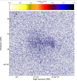
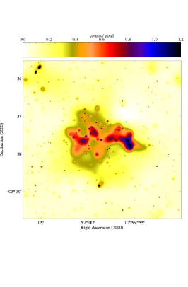
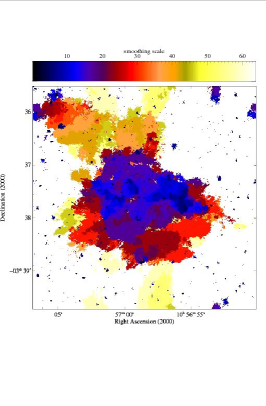
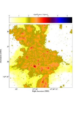
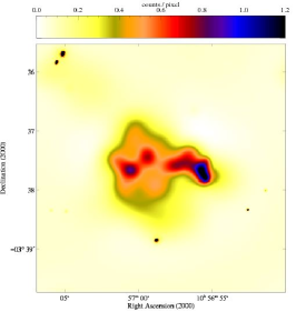
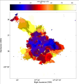
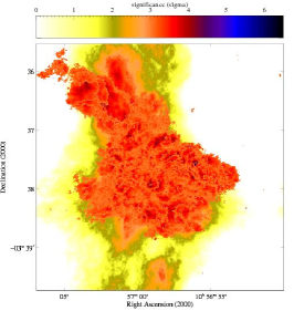
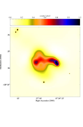
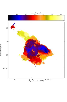
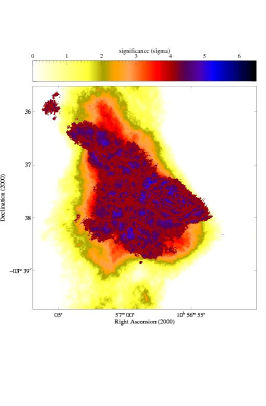
Fig. 1 (top left panel) shows the raw counts detected with ACIS-S in the 0.5 to 7 keV energy band in an 89 ks observation of the galaxy cluster MS 1054.4$-$0321. The diffuse emission originates from an electron-ion plasma trapped in the gravitational potential well of the cluster and heated to temperatures of typically $1\times 10^{8}$ K (corresponding to ${\rm k}T\approx 10$ keV). A detailed analysis of this observation is given by Jeltema et al. (2001). The image shown here ($512\times 512$ pixel²) covers a subsection of the detector spanning a $4.2\times 4.2$ arcmin² region; the pixel size of 0.492 arcsec corresponds roughly to one on-axis resolution element of the telescope-detector configuration. Note the high background throughout the image, caused by high-energy cosmic rays.

Fig. 1 summarizes asmooth results obtained with a Gaussian kernel, and for s.n.r. target values of $\tau_{\mbox{\scriptsize min}}=2,\,3,\,4$ and $\tau_{\mbox{\scriptsize max}}=\tau_{\mbox{\scriptsize min}}+1$, in a three-by-three array of plots below the image of the raw data.

4.1.1 asmoothed images

The left-most column of Fig. 1 shows the adaptively smoothed images for the three different $\tau_{\mbox{\scriptsize min}}$ values. Asmooth fully preserves the high information content of the raw data in the high-s.n.r. regions corresponding to bright, small-scale features, while at the same time heavily smoothing the low-s.n.r. regions of the image where the signal approaches the background value. Note, however, that for small values of $\tau_{\mbox{\scriptsize min}}$ (top row) the goodness of the local estimation of the signal above the background is relatively low and noise is not removed efficiently on all scales.

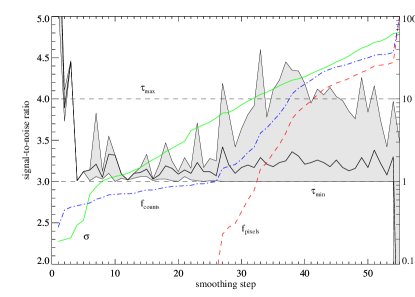
Figure 2 illustrates the gradual assembly of the adaptively smoothed image by showing the change in various asmooth parameters as a function of smoothing step.

At the highest pixel intensities above the s.n.r. threshold, asmooth occasionally returns smoothed count values that exceed the counts in the unsmoothed image: the brightest point source in the raw data has a peak value of 126 counts, the asmoothed image features a value of 128.5 at the same location. This is due to the fact that, although the corresponding pixels themselves remain essentially unsmoothed and thus keep their original values, there is an additional contribution from the larger sized kernels of neighbouring pixels whose s.n.r. above the background falls short of $\tau_{\mbox{\scriptsize min}}$. Since the final image is accumulated from the partial images resulting from the successive convolution with the whole set of differently sized kernels (cf. Eq. 10), the total smoothed intensity can become larger than the actually observed counts at pixel positions where $I(\vec{r}\,)\geq N_{\mbox{\scriptsize min}}$. This artifact is caused by the limited resolution of the images and can be noticeable when a large bin size is chosen for the original data. The integral number of counts in the image is always conserved.

Figure 2: Asmooth processing parameters as a function of smoothing step for one of the examples shown in the Fig 1 ($\tau_{\mbox{\scriptsize min}}=3,\,\tau_{\mbox{\scriptsize max}}=4$). The shaded region and solid black line delineate the range of signal-to-noise ratios and their median value, respectively, for the set of image pixels processed in each step. The target values $\tau_{\mbox{\scriptsize min}}$ and $\tau_{\mbox{\scriptsize max}}$ are marked by the dashed horizontal lines. Note the nonlinear increase in the smoothing radius $\sigma$ (green line), the cumulative fraction of pixels processed (red line), and the cumulative fraction of counts processed. Note also that the criterion of eq. 6 is a soft one as far as $N_{\rm max}$ ($\tau_{\rm max}$) is concerned: $\tau$ values greater than $\tau_{\rm max}$ are tolerated as long as the median value of the s.n.r. distribution for each smoothing step is smaller than $(\tau_{\rm max}+\tau_{\rm min})/2$. S.n.r. values exceeding $\tau_{\rm max}$ occur also at the smallest smoothing scales as the code is designed not to blur features whose s.n.r. is higher than $\tau_{\rm min}$ already in the raw data.

4.1.2 Kernel size and s.n.r. maps

As illustrated in Fig. 2 asmooth applies a wide range of smoothing scales to the input data as the algorithm attempts to fulfill the requirement given by Eq. 6 throughout the image. In addition to the adaptively smoothed image, asmooth also returns, in an IDL data structure, maps of the background-corrected s.n.r. of the pixel values in the smoothed image and the kernel size used in the smoothing process, respectively,

The second and third columns of the three-py-three panel in Fig. 1 show both of these maps for the asmooth images shown in the first, left-most column of plots. The maps of asmooth kernel sizes as well as Fig 2 demonstrate how very small kernel sizes of less than or about one pixel ($1\sigma$ radius) are assigned to very few bright pixels; accordingly, these pixels remain essentially unsmoothed. For $\tau_{\rm min}=3$ (middle row), for instance, some 27 per cent of the image pixels are found to satisfy the criterion of Eq. 6 at smoothing scales between one and 62 pixels (radius), while the majority of the remaining pixels (more than 72 per cent) do not contain enough signal to reach the required s.n.r. even at the largest permissible smoothing scale. The majority of the image is smoothed at the largest possible scale of 63.8 pixels at which the dimensions of the background kernel array (a 1$\sigma$ wide annulus surrounding the two-dimensional Gaussian smoothing kernel computed out to $3\sigma$ radius) equals that of the image itself. The s.n.r. maps (Fig. 1, right-most column), finally, give evidence of the near-constant s.n.r. of all regions smoothed with kernels other than the largest one.

4.1.3 Statistical properties of the residual image

Figure 3: The ratio of the variance of the residual signal to the mean (as given by the smoothed signal) as a function of the smoothed signal for the example shown in Fig. 1. Only bins containing at least 5 pixels are shown. Also shown are Gaussian errors based on the number of pixels per bin. For a perfect smoothing algorithm the plotted ratio is unity at all values of the mean. The bold lines (red, green, and blue) representing the results obtained with asmooth for $\tau_{\rm min}=2,\,3,$ and 4 come close to the ideal of a constant value of unity for most values of the mean. Only a few bright pixels exhibit significantly higher variance than expected for Poissonian statistics. By comparison, fixed kernel smoothing (see the fine solid lines) results in far too high variances for all but the smallest kernel size. Strong deviations from Poissonian statistics are observed over large portions of the image. The chosen fixed kernel sizes assume the values of the $1/100^{\rm th},\,3/100^{\rm th},\,1/10^{\rm th},\,1^{\rm st},$ and $10^{\rm th}$ percentile of the distribution of asmooth kernel sizes for $\tau_{\rm min}=3$ (1.1, 2.5, 6.7, 11.4, and 21.9 pixels).

The qualitative demonstration of the performance of asmooth shown in Fig. 1 can be made more quantitative by comparing it with the results obtained with fixed-kernel smoothing. To this end we examine the properties of the residual images obtained by subtracting the respective smoothed image from the observed raw image. Following Piña & Puetter (1992) who introduced this criterion in the context of Bayesian image reconstruction, we state that, for an ideal smoothing algorithm, this residual image should contain only uncorrelated Poissonian noise around a zero mean. A global mean of zero is guaranteed – within the numerical accuracy of the convolution code – by the requirement that any smoothing algorithm conserve counts. The requirements that the mean also be zero locally, that the residual signal have Poissonian variance, and that the residual signal be uncorrelated across the image are much harder to meet. In the following we shall examine how well adaptive and fixed kernel smoothing fulfill these requirements.

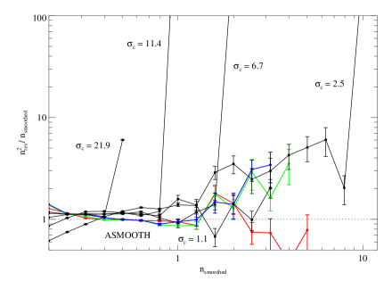
Is the residual signal consistent with Poissonian noise shifted to zero mean as expected if shot noise dominates?

If so, the square of the noise (given by the residual signal), $n_{\rm res}^{2}$, should equal the mean (given by the smoothed signal $n_{\rm smooth}$). Since the smoothed image contains a wide range of mean values, we can test for this condition only within bins of similar mean. Figure 3 shows the ratio $n_{\rm res}^{2}/n_{\rm smooth}$ as a function of $n_{\rm smooth}$ for both asmooth and a number of fixed kernels of various sizes. Note how the residual signal obtained with asmooth exhibits a near-Poissonian variance over a larger range of mean values than does the residual produced by smoothing with a fixed kernel of essentially any size. Only the smallest fixed kernel size tested here, $\sigma_{c}=1.1$ pixels, yields comparable results — a kernel of such small size, however, also provides essentially no smoothing.

Figure 4: The normalized autocorrelation function (cf. Eq. 12) of the signal in the residual images obtained by subtracting the smoothed image from the original one for the example shown in Fig. 1. For a perfect smoothing algorithm the autocorrelation signal is zero at all lags $r>0$. The almost indistuinguishable bold lines (red, green, and blue) representing the results obtained with asmooth for $\tau_{\rm min}=2,\,3,$ and 4 come close to this ideal at the price of a slight positive correlation on all scales. Fixed kernel smoothing always results in significant spatial correlations. The chosen fixed kernel sizes assume the values of the $1/100^{\rm th},\,3/100^{\rm th},\,1/10^{\rm th},\,1^{\rm st},$ and $10^{\rm th}$ percentile of the distribution of asmooth kernel sizes for $\tau_{\rm min}=3$ (1.1, 2.5, 6.7, 11.4, and 21.9 pixels).

Is the signal in the residual image spatially uncorrelated?

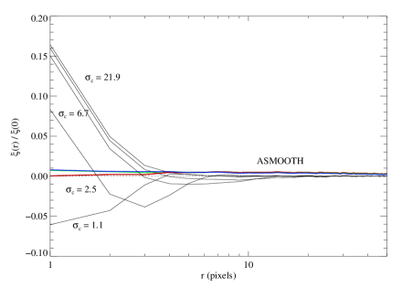
Figure 4 shows the autocorrelation function of the residual images obtained with asmooth and fixed kernels of various sizes. Here we use the standard definition of the autocorrelation $\xi$ as a function of radial lag $r$:

$$\xi(r)=\frac{\langle I_{\rm res}(\vec{r}\,^{\prime})\,I_{\rm res}(\vec{r}\,^{\prime}+\vec{r}\,)\rangle}{\langle I_{\rm res}\rangle^{2}}-1$$ (12)

where the angular brackets signify averaging over the position $\vec{r}\,^{\prime}$ within the image (e.g. Peebles 1980). In the normalized representation of $\xi(r)$ shown in Fig. 4 an ideal smoothing algorithm would produce zero signal at all lags except for a singular value of unity at $r=0$. Asmooth comes close to this ideal: the signal in the residual images generated with asmooth is essentially uncorrelated at all scales except for a weak ($\leq 2\%$) positive signal at scales smaller than about the maximum adaptive kernel size. Note the very different result when fixed Gaussian kernels of size $\sigma_{\mbox{\scriptsize const}}$ are used: strong spatial correlations are observed in the residual images at all scales smaller than about the kernel size. Only for very small kernel sizes does non-adaptive smoothing come close to meeting the requirement that any residual signal after smoothing be spatially uncorrelated. However, such small kernel sizes perform very poorly in the presence of significant structure on a large range of scales (cf. Fig. 1, center column).

4.2 Simulated data

The example shown in the previous section has the advantage of using real data but, for this very reason, does not allow the user to assess quantitatively how the asmoothed image compares to the true counts distribution underlying the noisy input image. We therefore present in this section results obtained for a simulated data set that contains multiple extended and point-like features, as well as a constant background component.

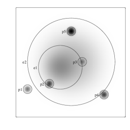
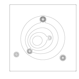
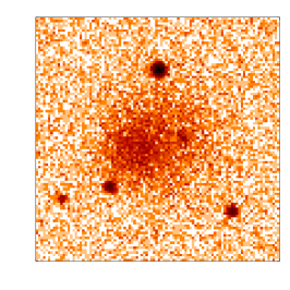
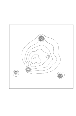
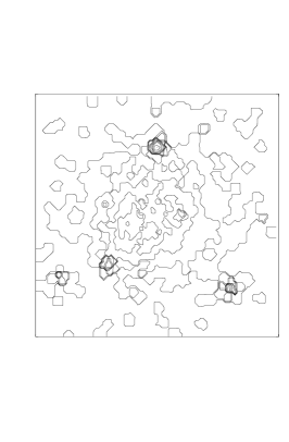
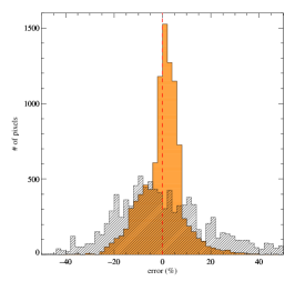
Figure 5 summarizes the characteristics of the model used for our simulation (top row). The same figure shows, in the bottom row, results obtained with Asmooth for $\tau_{\rm min}=3,\,\tau_{\rm max}=\tau_{\rm min}+1$, and with the adaptive binning algorithm WVT (Diehl & Statler 2005) for a target s.n.r. value of 5. Note how the requirement of a minimal s.n.r. above the local background (Eqs. 4 and 5) causes Asmooth to reduce noise much more aggressively than WVT in spite of a nominally lower s.n.r. target value. As demonstrated by the error distribution depicted in the final panel of Fig. 5 the asmooth residual image exhibits a near Gaussian error distribution around zero mean, in addition to featuring Poissonian variance and being spatially uncorrelated (Section 1). Asmoothed images can thus be considered to be fair representations of the ‘true’ input image.

Figure 5: Top row. Left: The model used in our simulation, a combination of two extended, four compact features, and a spatially invariant background component, designed to mimic an astrophysical X-ray image of point sources superimposed on asymmetric diffuse emission from, e.g. a cluster of galaxies. Center: Iso-intensity contours for the same model. Right: input image obtained by applying Poisson noise to the model. Bottom row. Left: Iso-intensity contours of the asmoothed image obtained with a Gaussian kernel and $\tau_{\rm min}=3$ – the contour levels are the same as above for the model image. Center: Iso-intensity contours of an adaptively binned image as obtained with the WVT algorithm (Diehl & Statler 2005) for an s.n.r. target value of 5 – the contour levels are again the same as for the model image. Note that, unlike asmooth, WVT does not correct for a local background in its s.n.r. estimation. Right: Histogram of relative errors, defined as (result – model)/model, in percent for Asmooth (solid orange fill) and the WVT adaptive binning code (hatched).

5 Summary

We describe asmooth, an efficient algorithm for adaptive kernel smoothing of two-dimensional image data. Asmooth determines the local size of the kernel from the requirement that, at each position within the image, the signal-to-noise ratio of the counts under the kernel, and above the background, must reach (but not exceed greatly) a certain preset minimum. Qualitatively, this could be called the ‘uniform significance approach’. As a consequence of this criterion, noise is heavily suppressed and real structure is enhanced without loss of spatial resolution. Due to the choice of boundary conditions, the algorithm preserves the total number of counts in the raw data. The asmoothed image is a fair representation of the input data in the sense that the residual image is consistent with pure noise, i.e., it the residual possesses Poissonian variance and is spatially uncorrelated. As demonstrated by the results obtained for simulated input, the adaptively smoothed images created by Asmooth are fair representations of the true counts distribution underlying the noisy input data.

Since the background is accounted for in the assessment of any structure’s s.n.r., a feature that distinguishes asmooth from most other adaptive smoothing or adaptive binning algorithms, the interpretation of the adaptively smoothed image is straightforward: all features in the asmoothed image are equally significant at the scale of the kernel used in the smoothing. A map of these smoothing scales is returned by asmooth together with the smoothed image. Note that these are the smallest scales at which real features reach the selected s.n.r. threshold. Consequently, background regions never meet the s.n.r. criterion and are smoothed at the largest possible scale for which the kernel size equals the size of the image. Such regions of insufficient signal are easily flagged using an s.n.r. map which is also provided by our algorithm.

We emphasize that our definition of “signal” as meaning “signal above the (local) background” was chosen because many, if not most, real-life appplications do not provide the user with a priori knowledge of the intensity of the background or any spatial background variations. Also, superpositions of features (such as the point sources on top of diffuse emission in our Chandra ACIS-S example) require a local background estimate if the intrinsic signal of features on very different scales is to be assessed reliably. The approach taken by Asmooth is thus intrinsically very different from the one implemented in, for instance, the adaptive binning algorithm WVT (Diehl & Statler 2005) and the difference in the resulting output is accordingly dramatic (see Section 4.2).

Asmooth is being used extensively in the analysis of astronomical X-ray imaging data gathered in a wide range of missions from ROSAT to XMM-Newton, and has become the analysis tool of choice for the display of high-resolution images obtained with the Chandra X-ray observatory. Recent examples illustrating asmooth’s performance can be found in Ebeling, Mendes de Oliveira & White (1995), Brandt, Halpern & Iwasawa (1996), Hamana et al. (1997), Ebeling et al. (2000), Fabbiano, Zezas & Murray (2001), Krishnamurthi et al. (2001), Karovska et al. (2002), Bauer et al. (2002), Gil-Merino & Schindler (2003), Heike et al. (2003), Rasmussen, Stevens & Ponman (2004), Clarke, Blanton & Sarazin (2004), Ebeling, Barrett & Donovan (2004), or Pratt & Arnaud (2005), as well as in many Chandra press releases (http://chandra.harvard.edu/press/).

Under development is an improved version of the algorithm which accounts for Poisson statistics using the analytic approximations of Ebeling (2003) to allow proper treatment of significant negative features, such as absorbed regions, detector chip gaps, or instrument elements (e.g., the window support structure of the ROSAT PSPC) obscuring part of the image.

Asmooth is written in the IDL programming language. The source code is available on request from ebeling@ifa.hawaii.edu. A $C++$ version of an early version of the code, called csmooth, is part of CIAO, the official suite of data analysis tools for the Chandra X-ray observatory, and is not identical to the algorithm described here.

References

- [1] Bauer F.E. et al. 2002, AJ, 123, 1163
- [2] Brandt W.N., Halpern J.P. & Iwasawa K. 1996, MNRAS, 281, 687
- [3] Ebeling H., Mendes de Oliveira C. & White D.A. 1995, MNRAS, 277, 1006
- [4] Cappellari M. & Copin Y. 2003, MNRAS, 342, 345
- [5] Clarke T.E., Blanton E.L. & Sarazin C.L. 2004, 616, 178
- [6] Diehl S. & Statler T.S. 2005, MNRAS, submitted
- [7] Ebeling H. et al. 2000, ApJ, 534, 133
- [8] Ebeling H. 2003, MNRAS, 340, 1269
- [9] Ebeling H., Barrett E. & Donovan, D. 2004, ApJ, 609, L49
- [10] Fabbiano G., Zezas A. & Murray S.S. 2001, ApJ, 554, 1035
- [11] Gil-Merino R. & Schindler S. 2003, A&A, 408, 51
- [12] Hamana T., Hattori M., Ebeling H., Henry J.P., Futamase T., Shioya Y. 1997, ApJ, 484, 574
- [13] Heike K., Awaki H., Misao Y., Hayashida K., Weaver K.A. 2003 ApJ, 591, 99L
- [14] Huang Z. & Sarazin C. 1996, ApJ, 461, 622
- [15] Jeltema T.E., Canizares C.R., Bautz M.W., Malm M.R., Donahue M., Garmire G.P. 2001, ApJ, 562, 124
- [16] Karovska M., Fabbiano G., Nicastro F., Elvis M., Kraft R.P., Murray S.S. 2002, ApJ, 2002, 577, 114
- [17] Krishnamurthi A., Reynolds C.S., Linsky J.L., Martin E., Gagné M. 2001, AJ, 121, 337
- [18] Lorenz H., Richter G.M., Capaccioli M., Longo G. 1993, A&A, 277, 321
- [19] Merritt D. & Tremblay B. 1994, AJ, 108, 514
- [20] Peebles P.J.E. 1980, The Large-Scale Structure of the Universe, Princeton, Princeton University Press
- [21] Piña R.K. & Puetter R.C. 1992, PASP, 104, 1096
- [22] Pisani A. 1993, MNRAS, 265, 706
- [23] Pisani A. 1996, MNRAS, 278, 697
- [24] Pratt G.W. & Arnaud M. 2005, A&A, 429, 791
- [25] Rasmussen J., Stevens I.R. & Ponman T.J. 2004, MNRAS, 354, 259
- [26] Richter G.M., Bohm P., Lorenz H., Priebe A. 1991, Astron. Nachr., 312, 346
- [27] Sanders J.S. & Fabian A.C. 2001, MNRAS, 325, 178
- [28] Silverman B.W. 1986, Density Estimation for Statistics and Data Analysis, Chapman & Hall, London
- [29] Starck J.-L. & Pierre M. 1998, A&AS, 128, 397
- [30] Thompson A.M. 1990, A&A, 240, 209
- [31] Vio R., Fasano, G., Lazzarin M., Lessi, O. 1994, A&A, 289, 640