Hybrid Estimation of CMB Polarization Power Spectra
Abstract
This paper generalises the hybrid power spectrum estimator developed in Efstathiou (2004a) to the estimation of polarization power spectra of the cosmic microwave background radiation. The hybrid power spectrum estimator is unbiased and we show that it is close to optimal at all multipoles, provided the pixel noise satisfies certain reasonable constraints. Furthermore, the hybrid estimator is computationally fast and can easily be incorporated in a Monte-Carlo chain for Planck-sized data sets. Simple formulae are given for the covariance matrices, including instrumental noise, and these are tested extensively against numerical simulations. We compare the behaviour of simple pseudo- estimates with maximum likelihood estimates at low multipoles. For realistic sky cuts, maximum likelihood estimates reduce very significantly the mixing of and modes. To achieve limits on the scalar-tensor ratio of from sky maps with realistic sky cuts, maximum likelihood methods, or pseudo- estimators based on unambiguous and modes, will be essential.
Key words: Methods: data analysis, statistical; Cosmology: cosmic microwave background, large-scale structure of Universe
1 Introduction
In an earlier paper (Efstathiou 2004a, hereafter E04) a hybrid power spectrum estimator was developed for temperature anisotropies of the cosmic microwave background (CMB) anisotropies. This estimator combined quadratic maximum likelihood (QML) estimates at low multipoles with a set of pseudo- (PCL) estimates at higher multipoles to produce a near optimal power spectrum estimate over the entire multipole range for realistic sky coverages, scanning patterns and instrument noise. We used analytic arguments and large numbers of numerical simulations to demonstrate that the method was near optimal and that the covariance matrix over the full range of multipoles could be estimated simply and accurately.
A full maximum-likelihood estimator would require the inversion and multiplication of matrices, where is the size of the data vector. For WMAP (Bennett et al. 2003a) or Planck (Bersanelli et al. 1996; The Planck Consortia 2005) sized data sets, with , a brute force application of methods is impossible computationally. This has been portrayed as a major computational challenge in CMB data analysis (e.g. Bond et al. 1999; Borrill 1999) and various approximate, but computationally demanding, techniques for solving this problem have been proposed (e.g. Oh, Spergel and Hinshaw 1999, Doré, Knox and Peel (2001), Pen 20003). One of the major motivations for E04 was to show that an computation is unnecessary and that a near-optimal estimator (essentially indistinguishable from an exact maximum-likelihood solution), with a calculable covariance matrix, could be estimated simply by combining PCL and QML estimates. Furthermore, the analysis of realistic experiments must deal with uncertainties such as correlated instrument noise, beam calibrations, foreground separation, point sources etc. It is simply not worth performing an exact power spectrum analysis if the assumptions under which it is optimal are violated by ‘real world’ complexities, and if these complexities cannot be folded into the error estimates. With a fast hybrid estimator it is feasible to assess such ‘real-world’ complexities using a hybrid estimator within a Monte-Carlo chain and to quantify any corrrections to the covariance matrix, or likelihood function. The ability to analyse such ‘real-world’ effects is likely to be much more important than any hypothetical marginal improvement that might be gained by applying a full method. We refer the reader to E04 for a discussion of the rationale for a hybrid estimator. The arguments will not be repeated here. Instead, we will focus on generalising E04 to the estimation of power spectra of the CMB polarization anisotropies.
As is well-known, the Thomson scattering of an anisotropic photon distribution leads to a small net linear polarization of the CMB anisotropies (for an introductory review and references to earlier work see Hu and White 1997). This polarization signal can be decomposed into scalar -modes and pseudo-scalar -modes. The separation of a polarization pattern into and modes is of particular interest since scalar primordial perturbations generate only mode while tensor perturbations generate and modes of roughly comparable amplitudes (Zaldarriaga and Seljak 1997; Kamionkowski, Kosowsky and Stebbins 1997). The detection of an intrinsic -mode signal in the CMB would provide incontrovertible evidence that the Universe experienced an inflationary phase and would fix the energy scale of inflation (see e.g. Lyth 1984).
An -mode polarization signal was first discovered by DASI111 Degree Angular Scale Interferometer (Kovac et al. 2002, Leitch et al. 2004). Exquisite measurements of the temperature--mode (TE) cross power spectrum have been reported by the WMAP222Wilkinson Microwave Anisotropy Probe team (Kogut et al. 2003). Measurements of the -mode power spectrum have been reported by the CBI333Cosmic Background Imager experiment (Readhead et al. 2004) and by the 2003 flight of Boomerang (Montroy et al. 2005). Primordial -mode anisotropies have not yet been detected in the CMB. The detection of -mode and possibly -mode anistropies is one of the main science goals of the Planck mission and of ground based experiments such as Clover (Taylor et al. 2004).
Associated with these experimental developments, there have been many investigations of techniques for analysing and modes from maps of the CMB sky. These analyses can be grouped, approximately, into the following catagories:
-
(i)
PCL estimators and correlation functions: Fast methods of estimating and -mode power spectra using correlation functions are described by Chon et al. (2004). Statistically equivalent PCL estimators are described by Kogut et al. (2003), Hansen and Gorski (2003), Challinor and Chon (2005, hereafter CC05) and Brown et al. (2005). In particular, CC05 present analytic approximations to the covariance matrices of PCL estimates for the case of noise-free data, while Brown et al. (2005) develop a Monte-Carlo method for calibrating covariance estimates from incomplete maps of the sky. PCL estimators can be evaluated using fast spherical transforms and hence scale as .
-
(ii)
Maximum Likelihood Methods: The generalization of the iterative maximum likelihood power spectrum estimation methods of Bond et al. (1998) to the analysis of polarisation is straightforward and will not be discussed further here. Tegmark and de Oliveira-Costa (2001, hereafter TdO01) define a quadratic estimator which is based on assumed forms for the temperature and polarization power spectra, generalising earlier work of Tegmark (1997). This method, which we will refer to as QML, is equivalent to a maximum likelihood solution if the guesses for the power spectra are close to their true values. As explained above, these methods involve matrix inversions and multiplications which scale as .
-
(iii)
Harmonic and Mode Decomposition: The Stokes’ parameters and describing linear polarization define a rank two symmetric trace-free polarization tensor on sphere. Over the complete sky, the polarization tensor can be decomposed uniquely into and modes. However, since the and decomposition is non-local, it is non-unique in the presence of boundaries. In any realistic situation, a sky cut must be imposed to exclude contamination of the CMB signal by high levels of Galactic emission at low Galactic latitudes. Various authors have discussed ways of detecting pure and modes from and maps on an incomplete sky (Lewis et al. 2002; Bunn et al. 2003; Bunn 2003; Lewis 2003). A key motivation for these analyses has been for diagnostic purposes (e.g. checking for a frequency dependent Galactic -mode signal). However, as this article was nearing completion an interesting paper appeared by Smith (2005) describing how to construct pseudo- estimators from unambiguous and modes on a cut sky. This type of analysis can effectively eliminate the severe and mode mixing that afflicts simple pseudo- estimators at low multipoles (see Section 3.4). (The method is not completely straightforward, nor unique, because it requires a ‘pre-estimation’ step to define unambiguous modes. We will throughout this paper use the abbreviation PCL to refer to the simple pseudo- estimators as defined in Section 2.)
As we will show in this paper, these three analysis techniques are closely related. To illustrate how these methods are interelated it is useful to consider separately the cases of noise-free and noisy data:
Comparison of PCL and QML estimators for noise-free data: On a complete sky with noise-free data, PCL and QML estimates are identical. However, a sky cut will couple CMB modes over a range of multipoles , and this will lead to mixing of and pseudo-multipoles defined over the incomplete sky (see Section 2). Although PCL power spectrum estimators can be defined which give unbiased estimates of the true and mode power spectra in the mean, the mixing of and modes is reflected in large variances and couplings between the estimated power spectra at multipoles (Section 2). A QML estimator applied to noise-free data unscrambles the - and -mode multipoles, in much the same way as the direct modal decompositions described by Lewis et al. (2002), Lewis (2003) and Smith (2005). The QML estimator returns almost optimal power spectrum estimates with smaller variances than a PCL estimator (Section 3). In particular, for realistic sky cuts an estimator that minimises and mode mixing, such as the QML estimator, is essential if one wants to probe low amplitude -mode signals (tensor-scalar ratios ). At high multipoles, , and mode mixing becomes unimportant and, in the case of noise free data, QML and PCL estimators become statistically equivalent (Section 3).
Comparison of PCL and QML estimators for noisy data: If the following conditions are satisfied: (a) the and maps have identical noise properties; (b) the noise is uncorrelated with variance per pixel ; (c) the estimates of and mode power spectra are for multipoles higher than some characterstic multipole , where noise dominates; then one can show that an inverse-variance weighted PCL estimator is statistically equivalent to a QML estimator (Section 4.2). For the intermediate multipoles, , the optimal weighting for PCL estimates is intermediate between equal weight per pixel and inverse variance weighting. By combining a set of PCL estimates with different weights, it is possible to define a fast polarization estimator (in analogy with the temperature estimator discussed by E04) that is statistically indistinguishable from a maximum likelihood estimator over a wide range of multipoles. Dealing with strongly correlated noise is more problematic. Fortunately, for Planck-type scanning strategies, the noise pattern (in , and ) should be accurately white at high multipoles (Efstathiou 2005). A detailed correlated noise model should therefore only be required at low multipoles. It is straightforward to include a model for correlated noise in a QML estimate at low multipoles, provided the pixel noise covariance matrix can be estimated for low resolution maps (Section 4.2).
The layout of this paper is similar to that for the temperature analysis presented in E04. PCL polarization estimates are discussed in Section 2 together with analytic approximations for covariances matrices in the absence of instrumental noise. The relationship of this work to the results presented in CC05 is discussed. Section 3 discusses QML polarization estimators for noise free data. A large set of numerical simulations is used to illustrate the effects of and mode mixing on an incomplete sky for both PCL and QML estimators. Section 4 discusses PCL and QML estimators including instrumental noise and Section 5 discusses a hybrid polarization power spectrum estimator. To keep the discussion simple, most of the analytic and numerical results presented in this paper refer to and mode power spectrum estimation. Our discussion of the temperature- mode cross power spectrum (denoted in this paper) is, intentionally, less complete since no new concepts are required for its analysis. Our conclusions are summarized in Section 6.
2 Estimation using Pseudo-
We begin by relating the and Stokes parameters (defined in direction with respect to a spherical coordinate system , ) and the spin two harmonics:
| (1) |
Note that the sign convention for polarization in this paper follows that of Zaldarriaga and Seljak (1997), which differs from the IAU convention (see Hamaker and Bregman 1996). The coefficients are related to the and mode multipole coefficients and by
| (2) |
If we have an incomplete sky, we can compute ‘pseudo-multipole’ coefficients , and by computing the following sums,
| (3a) |
| (3b) |
| (3c) |
where in equations (3b) and (3c)
| (4) |
is the area of pixel and is an arbitrary weight function with spherical transform
| (5) |
From these pseudo-multipole coefficients, we can form the following PCL power spectrum estimates
| (6) |
The expectation values of these PCL estimates are related to the true values , , , by
| (7) |
where the matrices , , etc are given by (Kogut et al. 2003)
| (8a) |
| (8b) |
| (8c) |
| (8d) |
and is the power spectrum of the weight function
| (9) |
(cf equation (5)). In the absence of parity violating physics in the early universe, the primordial and spectra should be identically zero. Even if there is no compelling motivation from fundamental physics, there may be other reasons for wanting to estimate these spectra, e.g. for consistency checks and to test for systematic errors. However, to keep the analysis as simple as possible, they will be not be included in this paper.
If the sky cut is small, then the matrix appearing in equation (7) will be non-singular and hence invertible. If this is the case, then unbiased estimates of the true power spectra can be formed from the PCL estimates by evaluating 444The notation here follows the notation introduced in E04. The expectation values of the hatted PCL estimates () (if they are well defined) are equal to the true power spectra. The expectation values of the tilde estimates () are given by convolutions of the true power spectra (equation 7).
| (10) |
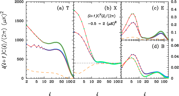
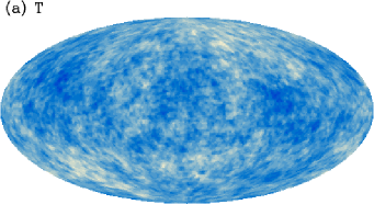
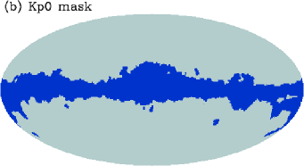
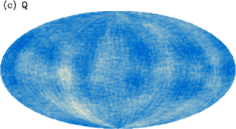
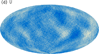
As an example, Figure 1 shows noise-free , and maps from a single Gaussian realisation of the concordance CDM model favoured by WMAP (Spergel et al. 2003). (The exact parameters adopted in this paper are those of the CDM model defined in Section 2 of Efstathiou (2003)). The maps have been created using software written by the author that uses an ‘igloo’ pixelisation scheme. The maps shown in Figure 1 have a pixel size of and a symmetrical Gaussian beam smoothing of FWMH of . In these simulations, we have assumed a tensor-scalar ratio of , where is defined in terms of the relative amplitudes of the ensemble averages of the temperature power spectra at ,
| (11) |
As in E04, unless otherwise stated, beam functions will not be written explicitly in equations and so will sometimes mean , where is the Gaussian beam function
| (12) |
Figure 1 also shows one of the Kpn family of WMAP masks (see Bennett et al., 2003b, for a discussion of the WMAP masks). The Kp0 mask shown in Figure 1 removes about 21 per cent of the sky at low Galactic latitudes and is a relatively conservative Galactic mask. (For reference, the WMAP TE analysis reported by Kogut et al. (2003) used the less conservative Kp2 mask which removes around 13 per cent of the sky).
Figure 2 shows the averages of PCL estimates and computed from noise-free simulations with the same cosmological parameters used to construct Figure 1 and with the Kp0 sky mask applied. For the Kp0 mask, the matrix in equation (10) is non-singular and can be inverted. Figure 2 shows that the PCL estimates provide unbiased estimates of the true power spectra.

For the temperature polarization power spectrum, accurate expressions for the covariance matrices of PCL power spectrum at high multipoles () can be derived quite easily (see E04). The analogous problem for polarization estimates is much more difficult (see CC05) because the covariances depend on the matrix products , , where
| (13) |
CC05 show that these products can be expressed as integrals as in equation (13), but with the window finction replaced by and integrals involving the gradients of . For PCL estimates from noise free data, the covariance matrices can therefore be approximated by terms which depend on the coupling matrices in equations (8a - 8d), but with replaced by the power spectrum of the square of the window function,
| (14) |
together with complicated terms that depend on gradients of the window functions .555There are no such gradient terms for the temperature covariance matrix , see E04 for a detailed analysis. Ignoring the gradient terms, the covariances can be approximated by
| (15a) |
| (15b) |
| (15c) |
| (15d) |
| (15e) |
The covariance matrix of the PCL estimates is given by
| (16) |
where is the matrix appearing in equation (7) (i.e. computed from , rather than from the power spectrum of ). Neglect of the gradient terms will be referred to somewhat loosely as the ‘scalar approximation’, since the expressions (15a-15e) depend on only the spin-0 multipoles of the square of the window function (14). It is interesting to ask under what circumstances the scalar approximation provides accurate estimates of the covariances. For relatively small sky cuts, such as the Kp0 mask, these expressions provide quite accurate estimates for the and power spectra at multipoles , where is the mode-coupling scale introduced by the sky cut. The left-hand panels in Figure 3 show the diagonal components of the covariance matrices for the , and power spectra estimated from equations (15b) - (15d) compared to estimates from the simulations used to generate Figure 2. For the Kp0 mask, the characterstic coupling scale is , and one can see from Figure 3 that the simple analytic expressions provide quite accurate estimates of the errors of the and power spectra at multipoles , but fail by a factor of or more for the component. The failure of simple analytic expression for the -component is related to mixing of the and modes. For the power spectrum, mixing of and modes is always unimportant at high multipoles, (since the -mode amplitude is fixed by the dominant scalar mode). We therefore expect the scalar approximation to provide accurate estimates of the covariances for the and power spectra at high multipoles. However, if the intrinsic amplitude of the mode is low, mixing of and modes can dominate the estimates of and the covariances and at high multipoles. For our chosen tensor-scalar amplitude, , mode-mixing dominates the amplitude at high multipoles, which is why the scalar approximation fails so badly.
Intuitively, one would expect that it would be possible to significantly reduce the effects of and mode mixing at high multipoles by apodising the sky cut. Apodisation down-weights data close to the edge where the non-local nature of the and mode decomposition causes ambiguity between modes (cf CC05). Thus we would expect the scalar approximation to be much more accurate if we apodise the Kp0 mask. Of course, in this context apodisation will lead to some information loss, but in practice the purpose of applying a mask is to reduce the effects of systematic errors caused by inaccuracies in modelling Galactic emission. Hence, the data close to the edge of a mask will usually be less reliable than data far removed from the mask. The slight loss of information caused by apodising is therefore likely to be more than compensated by the reduction in and mode mixing at high multipoles.
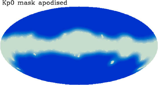
Figure 4 shows an example of an apodisation algorithm applied to the Kp0 mask. The apodisation algorithm works iteratively as follows. First, the Kp0 mask in this pixelisation is specified by or according to whether pixel lies within or outside the mask. Then:
(i) compute the spherical transform of the set of weights, , (equation 5) and multiply these coefficients by a smoothing factor of (equation 12) with Gaussian FWHM of ;
(ii) construct a smoothed weight function by performing an inverse spherical transform;
(iii) set the weights that lie within the original Kp0 mask equal to zero;
(iv) go back to step (i) and transform the smoothed weights to make a new set of coefficients and continue steps (i) – (iv) for a specified set of iterations.
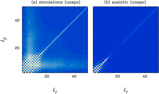
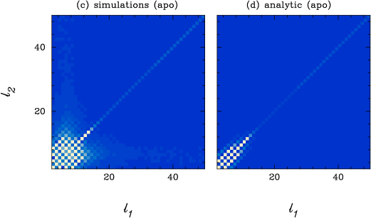
The example shown in Figure 4 shows the apodised mask after 4 iterations. The effective smoothing length therefore has a Gaussian FWHM of and one can see that the ‘islands’ interior to the masked region evident in Figure 1b have been smoothed to low amplitudes. The right-hand panels of Figure 3 show the diagonal components of the covariance matrices for the , and mode PCL power spectra of the apodised maps compared to the predictions of the scalar approximation. The and dispersions now agree almost perfectly with the scalar approximation for . For the mode, the variance caused by and mode mixing at is much less than for the unapodised case shown in Figure 3. For the diagonal components of the mode power spectrum, the scalar approximation is accurate to a few percent or so. Figure 5 shows the structure of the mode covariance matrices for the unapodised and the apodised Kp0 masks. In the apodised case, the covariance matrix is diagonally dominant at and the diagonal components are accurately described by equation (15d).
The scalar approximation is therefore a very good approximation for all three power spectra , and . Of course, even with apodisation, the scalar approximation for the mode spectrum will fail at some critical value of the tensor-scalar ratio , hence one cannot simply rescale equation (15d) by the appropriate amplitude of for arbitrarily low values of . For low values of , one can explicitly include the gradient terms which depend on the amplitude of (equation (80) of CC05) to get an accurate model of the covariance matrix at high multipoles. However, for most forseable experiments, including Planck, instrument noise is likely to dominate the -mode covariance matrix at high multipoles. In Section 4 we will show that in this situation the scalar approximation is extremely accurate independent of the intrinsic amplitude of .
3 Quadratic Maximum Likelihood
3.1 Preliminaries
A QML estimator for temperature CMB power spectra is discussed by Tegmark (1997). The generalization of this estimator to the estimation of CMB polarization is straightforward and is discussed in detail by TdO01. The estimator will be reviewed here briefly. We work in pixel space and define an input data vector consisting of the temperature differences and Stokes parameters and (defined with respect to a fixed coordinate system, as in Figure 1) specified at each pixel,
| (17) |
The optimal QML power spectrum estimate is (TdO01)
| (18) |
where the matrices are given by
| (19) |
and is the covariance matrix of the data vector ,
| (20) |
The matrices defined in equation (19) give formally minimum variance power spectrum estimates if the covariance matrix is set equal to the true covariance matrix. However, as noted by TdO01, equation (18) mixes components of the data vector with and components in providing estimates of the and mode power spectra. This is undesirable because for realistic noisy data, systematic errors in the measurements could contaminate estimates of the much lower amplitude and mode power spectra. It is therefore safer to separate the measurements from the and measurements by ‘reshaping’ the matrix (20):
| (21) |
and using the matrices
| (22) |
in place of the matrices in equation (18). The estimates will give unbiased estimates of the true power spectra , ,
| (23a) |
where
| (23b) |
By reshaping the covariance matrix, the estimate (18) will no longer be minimum variance. However, it is straightforward to show that for a Kp0-type mask, the increase in variance caused by using (21) instead of (20) is almost imperceptible.
Following E04 it is useful to define re-scaled power spectra
| (24) |
which have similar shapes to the true power spectra . Furthermore, if the matrix is invertible, one can define unbiased estimates of the true power spectra via
| (25) |
These estimators can be considered the QML analogues to the PCL estimators defined by equations (6) and (10).
The covariance matrices of the QML estimates is given by
| (26) |
where is the Fisher matrix. From equation (25), the covariance matrix of the deconvolved QML estimates is given by
| (27) |
Notice that if we had used the true pixel covariance matrix (20), rather than the ‘reshaped’ form (21), the covariance matrix (26) would take the more familiar form
| (28) |
Notice also from equations (18) and (22) that the estimator can be written as
| (29) |
where the are the PCL power spectra as defined in equation (6) but computed from the maps
| (30) |
( in equation (29) is the solid angle of a single map pixel, all assumed to be of identical area) Thus, if one can invert the matrix , the QML estimator can be computed rapidly by applying fast spherical transforms to the maps defined by equation (30). This is particularly useful if one wants to compute Monte-Carlo simulations of the QML estimator to characterise the covariance matrix. For applications to maps with large numbers of pixels, it may well be more efficient to use Monte-Carlo simulations to estimate errors, rather than brute force evaluation of (26), particularly if the covariance matrix (27) is accurately band diagonal (which is true for Kp0-like sky masks, see Figure 7 below).
3.2 Covariance Matrix at High Multipoles
In this Section, we will assume that and derive an approximation to the covariance matrix of for high multipoles and a small sky-cut. The analysis presented here is similar to the analysis of the QML temperature power spectrum covariance matrix given in Section 3.4 of E04.
If the -mode is absent, all of the information on the polarization anisotropies is contained in the spin field . The spin field contains no additional information. We can therefore construct a quadratic estimator
| (31) |
where is as defined in equation (19) with,
| (32) |
where is an arbitrary pixel weight function. If the sky cut is small, it will be a good approximation to set the inverse of to
| (33) |
using the completeness and othogonality relations for the tensorial harmonics. Hence,
| (34) |
and the Fisher matrix (23b) is
| (35) | |||||
where is the coupling matrix of equation (8c). Equation (34) agrees with equation (15c) and shows that for small sky-cuts and noise-free data, the QML estimator at high multipoles () is statistically equivalent to the PCL estimator with equal weight per pixel.
The derivation given here is only valid in so far as the B-mode can be ignored and the sky cut is small enough (and the multipoles high enough) that the approximation (33) is accurate. It is not straightforward to generalise the analysis presented here to admixtures of and modes. Given the results of Section 2, we would expect that at high multipoles and low B-mode amplitudes, the QML estimator for the B-mode power spectrum will be statistically equivalent to a PCL estimator with suitably apodised sky masks. In other words, the QML estimator will self-consistently find the appropriate apodisation (via equation 30) for any given geometry to minimise and mode leakage at each multipole.
3.3 Covariance Matrix at Low Multipoles
Generalising the discussion in Section 3.3 of E04 to polarization, we can consider the vector to consist of the harmonic coefficients and measured from noise free data on the cut sky. These are related to the true harmonic coefficients and by a coupling matrix
| (36) |
where the integrals are defined in equation (13). Evidently, if the coupling matrix in equation (36) can be inverted, then the true power spectra can be reconstructed. However, if the power spectra extend to high values of and , then the coupling matrix will be singular for a finite sky cut, since it is impossible to reconstruct modes that lie entirely within the cut. Furthermore, the presence of boundaries leads to ‘ambiguous’ modes, i.e. modes which cannot be assigned as pure and modes. As discussed in the Introduction, various authors have investigated harmonic mode reconstruction from data on an incomplete sky (Lewis et al. 2002; Bunn et al. 2003; Lewis 2003). The analysis by Lewis (2003) is particularly relevant to the discussion because he shows how to construct projections of pure and modes for noise-free data with a Kp2 sky mask. For low values of , (, where is the characteristic width of the sky cut), the true and modes can be reconstructed accurately. (i.e. for suitably band-limited data the coupling matrix (36) is invertible. As in the case of temperature anisotropies discussed by E04, for noise-free data on a cut-sky the QML estimator will effectively invert the coupling matrix at low multipoles, reconstructing almost the true values of the and mode power spectra for the full sky. The covariance matrix of the QML estimators at low multipoles should therefore be given by cosmic variance, i.e. diagonal with components
| (37) |
At high multipoles, the variance of the QML estimates will increase above cosmic variance (as given by equation (35) for the E-mode) to
| (38) |
where is the fraction of the sky surveyed, reflecting the loss of information on modes within the sky cut. (See CC05 for the analogue of equation (38) for at high multipoles in the limit .) The expectations of equations (37) and (38) are borne out by the tests described in Sections 3.4 and 5.
3.4 Comparison of PCL and QML methods for the Kp0 mask
Using the ‘reshaped’ covariance matrix of equation (21), the problem of estimating and mode power spectra becomes decoupled from the problem of estimating and power spectra. We will therefore confine the discussion in this Section to the estimation of and mode power spectra using the QML methodology described in Section 3.1. To compare the QML and PCL methods we have performed a set of noise-free simulations of the concordance CDM model with pixels and a smoothing of . The Kp0 mask was applied, leaving active pixels out of a total of pixels over the full sky. For these simulations, the amplitude of the input mode power spectrum was set to zero. For the PCL estimates, the Kp0 mask was apodised as described in Section 2 (see Figure 4).
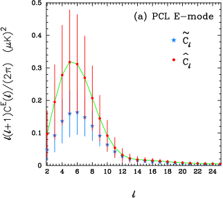
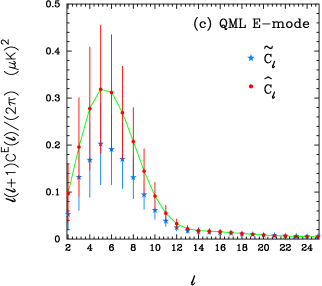
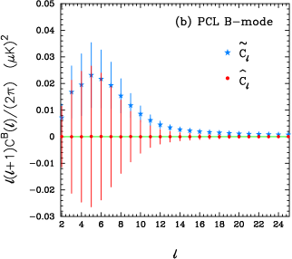
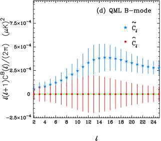
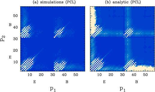
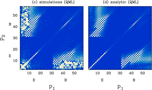
Results from these simulations are shown in Figures 6 and 7. Figure 6 shows that the deconvolved PCL and QML estimates provide unbiased estimates of the input power spectra. The errors of the -mode spectra are dominated by cosmic variance, though one can see that the Kp0 sky cut causes a noticeable increase in the PCL errors. This is equivalent to the discussion of ‘estimator induced’ variance for the temperature anisotropies at low multipoles discussed in Section 3.3 of E04 (see also Efstathiou 2004b). At low multipoles () the QML estimator returns very nearly the exact value of for each realisation and so the covariance matrix is accurately diagonal (Figures 7c and 7d) and limited by cosmic variance over the full sky (equation 37). In contrast, the PCL estimates of at low multipoles are strongly correlated (Figure 7a) as a result of the sky cut and have a large estimator-induced variance which amplifies the errors above those of the QML estimator.
The contast between the PCL and QML -mode estimates is even more extreme. The input -mode spectrum in these simulations is set to zero, thus any measured -mode is arising from mode leakage caused by the sky cut. From Figures 6b one can see that for the PCL estimator, leakage leads to -mode amplitudes of – , i.e. about of the amplitude of the -mode spectrum, simply as a result of the sky cut. The estimator induced variance is therefore huge and so even if one had noise-free data, it would not be possible to probe tensor-scalar ratios of using a Kp0 sky cut and PCL power spectrum estimates (see also CC05 for a similar conclusion). As expected from the discussion in Section 3.3, the QML estimator recovers almost the exact input power spectrum at low multipoles even on the cut sky. Thus in Figure 6d the QML -mode estimates have an amplitude of typically and the covariance matrix for these estimates is accurately diagonal (Figure 7d). The residual ‘estimator induced’ variance is a consequence of the coupling between low modes and high modes which limits the accuracy of an inversion of equation (36). Thus, for a Kp0-type sky cut the variance of the QML estimator leads to a limit on the detectability of a tensor-scalar ratio of in the absence of noise or residual foreground emission (see also Amarie, Hirata and Seljak 2005). It would be possible to probe lower values of by isolating pure -modes on the cut sky, as described by Lewis (2003), though methods for probing are probably only of academic interest at this stage, given our lack of knowledge of polarised foregrounds.
4 Including Instrumental Noise
4.1 PCL estimator with noise
In this Section we consider the effects of simple models of instrument noise. The data vector (17) is therefore split into a signal contribution and a noise contribution , which are assumed to be uncorrelated with covariance matrices and :
| (39) |
We assume further that the noise on each of the , and maps is uncorrelated. With these assumptions, the expectation values of the PCL power spectrum estimates is modified from (7) to
| (40a) |
| (40b) |
| (40c) |
| (40d) |
where the noise power spectra , and are given by
| (41a) |
| (41b) |
| (41c) |
If the noise covariance matrices are diagonal,
| (42) |
then the expressions (41a)-(41c) simplify to
| (42a) |
| (42b) |
where the last equation follows from the addition relation for tensorial harmonics,
| (43) |
and the angles () and () are related to the Euler angles () as described in Section 1.4.7 of Varshalovich, Moskalev and Khersonskii (1988).
Defining the coupling matrices,
| (44a) |
| (44b) |
| (44c) |
| (44d) |
for arbitrary , the analogues of equations (15a) - (15e) including uncorrelated instrumental noise in the case are:
| (45a) |
| (45b) | |||||
| (45c) |
| (45d) |
| (45e) |
where the various window functions appearing in equations (45a)–(45e) are defined by
| (46a) |
| (46b) |
| (46c) |
and
| (47) |

To check these expressions, we repeated the simulations described in Section 2 (i.e. , , ) but including uncorrelated noise with . With these noise levels, the -mode power spectrum is noise dominated for . PCL power spectrum estimates, using the apodised Kp0 mask of Figure 4, were computed for simulations.
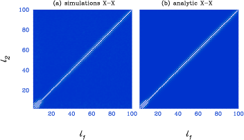
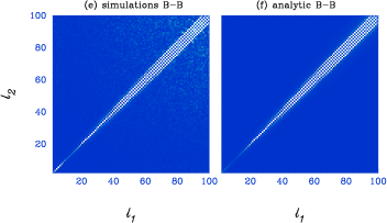
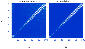
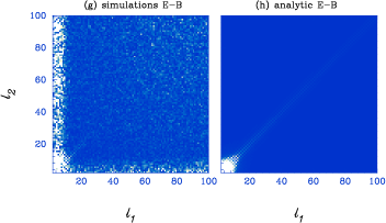
Figure 8 compares the diagonal components of the covariance matrices for the , and power spectra compared to the analytic expressions of equations (45b) – (45d). Apart from the addition of instrumental noise, these simulations are identical to those described in Section 2 and so Figure 8 can be compared directly with Figure 3. Figure 9 compares the full forms of the covariance matrices computed from the simulations to the analytic predictions of equations (45b) – (45e). Figures 8 and 9 show that that the scalar approximation is extremely accurate for all three spectra , and for . In the discussion of Figure 3, we pointed out that in the noise free case, the scalar approximation would break down for low tensor amplitudes (when the PCL B-mode amplitude is dominated by E-B mode mixing rather than true B modes). However, if the B-mode power spectrum is noise dominated at high multipoles (as it is in the simulations described in this Section), the covariance matrix is fixed by the pure noise term in equation (45d) which is independent of the amplitude of the intrinsic B mode. Thus in the noise dominated case, the scalar approximation will provide an accurate estimate of the PCL covariance matrices at high multipoles independent of the amplitude of the tensor component.
4.2 QML estimator with noise
Evidently, if the data vector includes instrumental noise, the generalization of equation (18) is,
| (48) |
and the covariance matrices in equations (19) and (20) are replaced by , where and are the signal and noise covariance matrices defined in equation (39).
If the noise is diagonal, , then in the noise dominated limit and one can see immediately from equation (30) that the QML estimator is mathematically equivalent to a PCL estimator applied to a map with inverse variance weighting, . As in the discussion of temperature power spectrum estimation (Hinshaw et al. 2003, E04), we find that the optimal weighting of a PCL estimator is:
(i) equal weight per pixel in the signal dominated limit;
(ii) inverse variance weighting in the noise-dominated limit, if the noise covariance matrix is diagonal.
As described in E04, one of the key motivations for a hybrid estimator is to construct an estimator that combines PCL power spectra computed with various weighting schemes to give a near optimal power spectrum estimate between the two extremes (i) and (ii). This intermediate regime is difficult to analyse analytically. The hybrid estimator is discussed in the next Section, which parallels closely the discussion for temperature anisotropies given in E04. There is, however, an important difference between the discussion of temperature and polarisation anisotropies. Consider, for example, the optimal inverse-variance weighted -mode pseudo-multipole,
| (49) |
Because of the spin nature of the polarisation anisotropies, it is not possible to derive simple expressions analogous to equation (7) relating PCL power spectra constructed from these multipoles to the true power spectra unless . If , one would need to evaluate (time-consuming) products of matrices to recover the true power spectra. For simplicity, we therefore assume in the rest of this paper, recognising that if this is not true, then it is not possible to define an easily computable optimal PCL estimator in the noise-dominated limit.
5 Hybrid Polarization Power Spectrum Estimator
Following E04, if we estimate a number of power spectra derived from the same data, where denotes the mode () and denotes the estimator (e.g. PCL estimates with different weight functions), then they can be combined into a single data vector from which we can define a ,
| (50) |
where is the hybrid estimator for mode , is the inverse of the covariance matrix . Minimising equation (50) gives the following linear equations, which we can solve to form the hybrid estimate
| (51) |
with covariance matrix
| (52) |
Evidently, since the hybrid estimator involves linear combinations of the power spectrum estimates , it will provide an unbiased estimate of the true power spectra, provided that each of the is unbiased. Nevertheless, as with the discussion of the optimal QML estimator in Section 3.1, the solution of (51) mixes power spectrum estimates for different modes, which may be undesirable in practice. For example, for PCL estimates, the covariance matrix is zero by symmetry, thus the PCL estimates and are strictly independent. However, the covariance matrices and are non-zero and are given by
| (53a) |
| (53b) |
where are the coupling integrals defined in equation (13) (with set to the weight function applied to the and maps) and is the coupling integral
| (53c) |
with set to the weight function applied to the temperature map. The calculation of the full solution of equation (51) is therefore complicated, and unless the errors are very well understood, there is a danger of introducing biases by mixing modes with very different amplitudes. Rather than use the strict minimum variance solution (51), it is preferable to ignore cross covariances and to compute for each mode separately the solution of
| (54) |
i.e.
| (55) |
The estimates (55) will be technically sub-optimal, but for practical purposes they will be indistinguishably close to optimal. The covariances and cross-covariances of the hybrid estimates are straightforward to compute and are given by
| (56) |
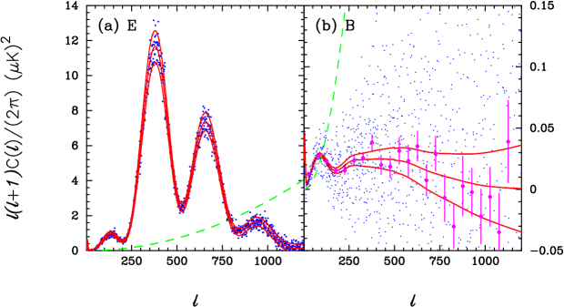
To illustrate the method, we generated a simulated sky of the concordance CDM cosmology with , at a pixel size of and with a Gaussian smoothing of . We simulated the hit-count distribution for a Planck-type scanning strategy as described in E04, i.e. a single detector pointing at to the spin axis of the spacecraft, and with the spin axis precessing slowly about the ecliptic plane according to , where is the ecliptic longitude. With this type of scanning strategy, regions with high hit counts are concentrated at the ecliptic poles as shown in Figure 11 of E04. The hit count distribution is normalised so that the mean hit count, is unity. Uncorrelated Gaussian noise was then added to the and maps with .
We concentrate on the analysis of the and power spectra in this Section. With these parameters, the and mode power spectra become noise dominated at at and respectively (see Figure 10). We apply an apodised Kp0 mask, as shown in Figure 4 but recomputed for the smaller pixels appropriate to these maps. In addition, a further weight factor was applied
| (57) |
as described in EO4, where is the noise level for a pixel in the or map with the mean hit count, and is the actual noise level in pixel . The parameter controls the weighting scheme so that corresponds to inverse variance weighting and corresponds to equal weight per pixel (apart from minor variations in the pixel areas associated with the pixelisation scheme).
The results plotted in Figure 10 show equation (55) applied to two sets of PCL estimates, one with equal weight per pixel and one with . (The cross-covariances between these estimates can be computed via a straigtforward generalisation of equations (45) – (47).) The solid lines in Figure 10 show the theoretical dispersion computed from the diagonal components of the covariance matrix (56). As can be seen from the scatter of the points, these estimates are entirely reasonable. In fact, in this example, the variances of the PCL estimates at high multipoles are relatively insensitive to the weighting scheme. At high multipoles, the weighting produces slightly (-) smaller errors compared to equal weight per pixel. However, in the signal dominated regime at low multipoles, the weighting gives much larger errors. This behaviour is similar to the behaviour for the temperature anisotropies illustrated in Figure 14 of E04.
To apply the QML estimator, the maps at high resolution were smoothed with a Gaussian beam of width and repixelised onto a low resolution map with pixel size . The QML estimator (48) requires the noise covariance matrix of the low resolution data. Since the noise in each high resolution map is diagonal, , the noise covariance matrix of a low resolution map is given by
| (58) |
where denotes the pixel number in the high resolution map, is the solid angle of pixel and is the Gaussian smoothing scale of the low resolution maps. In the small angle approximation, equation (58) simplifies to the easily computable expression
| (59) |
which is sufficiently accurate for the example discussed here.
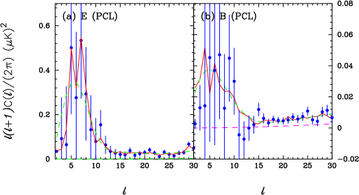
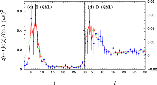
Figures 11a and 11b show the PCL estimates at low multipoles from Figure 10 on a greatly expanded scale. The error bars on the points show the dispersions computed from the diagonal components of the covariance matrix The solid (red) lines show the and -mode power spectra for this particular simulation and the (green) dashed lines show the theoretical power spectra of the concordance CDM model. The (purple) dashed line in Figure 11b shows the theoretical power spectrum of the noise.
Figures 11c and 11d show analogous plots for the QML estimator, corrected for the low resolution smoothing . In agreement with the tests shown in Figures 6 the errors on the QML estimates at low multipoles are considerably smaller than those for the PCL estimates. The covariance matrices for the QML estimates are very close to diagonal (c.f. Figure 7). Furthermore, the agreement between the and mode QML power spectrum estimates and the power spectra for this particular realisation (shown by the solid red lines), confirms the arguments given in Section 3.3 that the QML estimator will return almost the exact input power spectra even in the presence of a substantial sky cut. This is similar to the case of temperature power spectrum estimation, where a Kp0-like sky cut can introduce a substantial ‘estimator induced’ variance (Efstathiou 2004b) at low multipoles comparable to the cosmic variance (cf. Table 1 of Efstathiou 2004b). For polarization, however, the problem of estimator induced variance is particularly acute because of and -mode mixing. If the -mode amplitude is low, then the estimator induced variance of PCL estimators can easily overwhelm cosmic variance, whereas it is essentially negligible for a QML estimator. Notice that at multipoles – the PCL and QML estimates are closely similar (as expected from Section 3.2). At multipoles the errors on the QML estimates become larger than those of the PCL estimator because of the large smoothing applied to the low resolution maps. However, there is quite a wide range of multipoles over which the estimates and errors are almost identical. The pixel size and smoothing scale of the low resolution simulations used in this example was chosen for computational speed so that the QML code could be run quickly on a single processor workstation. It would be entirely feasible to extend the QML calculation to multipoles of a few hundred or more using modern multi-processor computers. For many realistic experimental configurations this would provide a large range of overlap with PCL estimates at high multipoles. Thus, in practice, it would be extremely accurate simply to combine PCL estimates using equation (55) and to overwrite the estimates at low multipoles, and associated components of the covariance matrices (56), with the corresponding QML estimates and covariance matrices.
Alternatively, one can calculate the cross-covariances between the QML estimates and PCL estimates, and include the QML estimates as part of the data vector used to compute the hybrid solution . One then requires estimates of the cross-correlations between the PCL and QML estimates. These are quite complicated, but for completeness, we give analytic expressions here for the case of noise-free data. If we write the QML estimates in the form
| (60) |
and define the quantities,
| (61a) |
| (61b) |
| (61c) |
| (61d) |
then the cross-covariances are given by
| (62a) |
| (62b) |
As explained above, for most purposes, it should be sufficiently accurate simply to overwrite PCL estimates and covariance matrices at low multipoles with those computed from QML, avoiding the complexity of evaluating equations (62a) and (62b).
6 Conclusions
This paper generalises the analysis of power spectrum estimators presented in E04 to the case of polarisation. Simple analytic expressions involving the power spectrum of the square of the window function (the scalar approximation) are given for the covariance matrices of PCL estimates, including the effects of uncorrelated instrument noise. For noise free data, the scalar approximation is shown to give accurate error estimates for the -mode power spectrum at high multipoles for realistic (Kp0-like) sky-cuts, and also for the -mode power spectrum provided the Q and U maps are apodised appropriately and the amplitude of the -mode is high enough. For noise dominated data, the scalar approximation povides extremely accurate covariance estimates for both the and modes at high multipoles.
The results presented in Section 3 establish certain relationships between QML and PCL estimators, in particular, the statistical equivalence of QML and PCL estimators in the noise-free and noise-dominated limits. This analysis parallels the discussion of temperature power spectrum estimates given in E04. However, in the noise-dominated limit, an optimal PCL polarization estimator can only be constructed for the special case of uncorrelated noise and identical noise levels in the Q and U maps, . Fortunately, for a Planck-type experiment, both of these assumptions should be reasonably accurate at high multipoles.
An analytic discussion of the noise properties of CMB temperature maps for a Planck-like scanning strategy with realistic ‘’ noise is given by Efstathiou (2005). For a Planck-type experiment, the noise should be accurately white at high multipoles (see also Stompor and White, 2004). Low frequency ‘’ noise introduces striping in the maps with a characterstic spectrum that varies approximately as at low multipoles. This low frequency behaviour for the temperature power spectra has been verified in many simulations of Planck-like experiments (e.g. Burigana et al. 1997, Maino et al. 1999; Keihänen et al. 2004; Efstathiou 2005). It is also seen in the , and power spectra from full-scale simulations of the polarised Planck GHz detectors (Ashdown et al. 2006).
For the knee-frequencies666The characteristic frequency above which the detector noise is approximately white. and noise levels expected of Planck detectors, the noise power spectra for both temperature and polarization will be accurately white-noise above multipoles of . For the temperature power spectrum, the effect of residual striping errors on the power spectrum at multipoles should be negligible, and so it should be an excellent approximation to treat the noise as pure white-noise. However, the simulations of Ashdown et al. (2005) show that the effects of striping errors on the and -mode power spectra at low multipoles will be comparable to (or will dominate) the intrinsic signal. These errors should therefore be folded into estimates of the power spectrum covariance matrices. This can be done by evaluating the QML estimator on low resolution maps, provided one can adequately approximate the noise covariance matrices for these low resolution maps. In Section 5 we showed that it is easy to compute for a low resolution map if the noise is strictly uncorrelated. However, the analogous problem for Planck-like correlated noise has not yet been solved and is currently under investigation.
Since the noise for a Planck-like experiment is accurately white at some characteristic multipole, a hybrid estimator based on PCL estimates at high multipoles and QML estimates at low multipoles, is well motivated. Furthermore, by applying a QML estimator at low multipoles, it is possible to eliminate almost completely the troublesome effects of and mode mixing associated with sky cuts. We have previously argued (E04, Efstathiou 2004b) that maximum likelihood estimators should be used to determine the temperature power spectrum at low multipoles on a cut sky to eliminate the large ‘estimator-induced’ variance inherent to PCL estimators. The problem of estimator-induced variance is even more acute for PCL estimators of the polarization power spectra (cf CC05). In particular, for the PCL estimators discussed here, mode-mixing places significant limits on the amplitude of the tensor-to-scalar ratio, , that can be probed even in a noise-free experiment. For example, the tests described in Section 3.4 show that it is difficult to probe below using a PCL estimator applied to maps with a Kp0 sky-cut. As Smith (2005) has shown, it is possible to define fast estimators based on unambiguous and modes on a cut sky. However, applying a QML estimator to low (or intermediate) resolution maps is also fast and is very close to optimal. In fact, if one wants to incorporate QML power spectrum estimation into a Monte-Carlo chain, then as equation (29) shows, the time taken to evaluate a QML power spectrum is no greater than the time taken to evaluate a fast spherical transform.
Acknowledgements: I thank members of the Cambridge Planck Analysis Centre, especially Mark Ashdown and Anthony Challinor, for helpful discussions.
References
- [AHS2005] Amarie M., Hirata C., Seljak U., 2005, astro-ph/0508293.
- [Aetal2006] Ashdown M.A.J., et al., 2006, in preparation.
- [Betal03a2003] Bennett, C. et al., 2003a, ApJS, 148, 1.
- [Betal03b2003] Bennett, C. et al., 2003b, ApJS, 148, 97.
- [Betal961996] Bersanelli M. et al., 1996, COBRAS/SAMBA Report on the Phase A Study. ESTEC.
- [Betal991999] Bond J.R., Crittenden R.G., Jaffe A.H., Knox L., 1999, Comput. Sci .Eng., 1, 21.
- [BJK981998] Bond J.R., Jaffe A.H., Knox L., 1998, PRD, 57, 2117.
- [B99b1999] Borrill J., 1999, in EC-TMR Conf. Proc. 476, 3K Cosmology, eds. L. Maiani, F. Melchiorri and N. Vittorio, Woodbury AIP, 277.
- [BCT052005] Brown M.L., Castro P.G., Taylor A.N., 2005, MNRAS, 360, 1262.
- [B032003] Bunn E.F., 2003, New Astron. Reviews, 47, 987.
- [BZTO032003] Bunn E.F., Zaldarriaga M., Tegmark M., de Oliveira-Costa A., 2003, PRD, 67, 023501.
- [BMMDMBM971997] Burigana C., Malaspina M., Mandolesi N., Danese L., Maino D., Bersanelli M., Maltoni M., 1997, Internal Report ITESRE. astro-ph/9906360.
- [CC052005] Challinor A.D., Chon G., 2005, MNRAS, 360, 509. (CC05)
- [CCPHS042004] Chon G., Challinor A., Prunet S., Hivon E., Szapudi I., MNRAS, 350, 914.
- [DKP012001] Doré O., Knox L., Peel A., 2001, PRD, 64, 3001.
- [E03a2003] Efstathiou G., 2003, MNRAS, 346, L26.
- [E042004] Efstathiou G., 2004a, MNRAS, 349, 603. (E04)
- [E04b2004] Efstathiou G., 2004b, MNRAS, 348, 885.
- [E052005] Efstathiou G., 2005, MNRAS, 356, 1549.
- [HB961996] Hamaker J.P., Bregman J.D., 1996, A&AS, 117, 161.
- [HG032003] Hansen F.K., Górski K., 2003, MNRAS, 343, 559.
- [Hetal032003] Hinshaw G. et al. 2003, ApjS, 148, 135.
- [HW971997] Hu W., White M., 1997, New Astronomy, 2, 323.
- [KKS971997] Kamionkowski M., Kosowsky A., Stebbins A., 1997, PRD, 55, 7368.
- [KKPMB042004] Keihänen E., Kurki-Suonio H., Poutanen T., Maino, D., Burigana C., 2004, A&A, 428, 287.
- [Ketal032003] Kogut A., et al., 2003, ApJS, 148, 161.
- [Ketal022002] Kovac J. M., Leitch E. M., Pryke C., Carlstrom J. E., Halverson N. W., Holzapfel W. L., 2002, Nature, 420, 772.
- [Letal022002] Leitch E. M. et al. Nature, 420, 772.
- [L032003] Lewis A., 2003, PRD, 68, 083509.
- [LCT022002] Lewis A., Challinor A., Turok N., 2002, PRD, 65, 023505.
- [L841984] Lyth D.H., 1984, Phys Lett B., 147, 403L.
- [OSH991999] Oh S.P., Spergel D.N., Hinshaw G., 1999, ApJ, 510, 551.
- [Metal991999] Maino D., et al., 1999, A&A Suppl. Ser., 140, 383.
- [Metal052005] Montroy T.E. et al., 2005, astro-ph/0507514.
- [P032003] Pen U.L., 2003, MNRAS, 346, 619.
- [Retal042004] Readhead A.C.S., et al. 2004, Science, 306, 836.
- [S052005] Smith K. M., 2005, submitted to PRD. astro-ph/0511629.
- [Setal032003] Spergel D.N., et al., 2003, ApJS, 148, 175.
- [S042004] Stompor R., White M., 2004, A&A, 419, 783.
- [T042004] Taylor, A.C. et al., 2004, To appear in the proceedings of the XXXVIXth Rencontres de Moriond ”Exploring the Universe, astro-ph/0407148.
- [T971997] Tegmark M., 1997, PRD, 55, 5895.
- [TdO972001] Tegmark M., de Oliveira-Costa A., 2001, PRD, 64, 063001. (TdO01)
- [PC052005] The Planck Consortia, 2005, The Scientific Programme of Planck, Efstathiou G., Lawrence C., Tauber J. (eds), ESA-SCI(2005)-1, ESA Publications.
- [VMK881988] Varshalovich, D.A., Moskalev A.N., Khersonskii V.K., 1988, Quantum Theory of Angular Momentum, World Scientific, Singapore.
- [ZS971997] Zaldarriaga M., Seljak U., 1997, PRD, 55, 1830.