Exponential Cardassian Universe

Abstract

The expectation of explaining cosmological observations without requiring new energy sources is forsooth worthy of investigation. In this letter, a new kind of Cardassian models, called exponential Cardassian models, for the late-time universe are investigated in the context of the spatially flat FRW universe scenario. We fit the exponential Cardassian models to current type Ia supernovae data and find they are consistent with the observations. Furthermore, we point out that the equation-of-state parameter for the effective dark fluid component in exponential Cardassian models can naturally cross the cosmological constant divide $w=-1$ that observations favor mildly without introducing exotic material that destroy the weak energy condition.

, ,

1 Introduction

The current accelerating expansion of the universe indicated by the astronomical measurements from Supernovae type Ia (SNeIa) [1] (see [2, 3] for most recent results) as well as accordance with other observations such as the cosmic microwave background (CMB) [4] and galaxy power spectra [5] becomes one of the biggest puzzles in the research field of cosmology. There are lots of approaches to unriddle this puzzle. One popular theoretical explanation approach is to assume that there exists a mysterious energy component, dubbed dark energy, with negative pressure, or equation of state with $w=p/\rho<0$ that currently dominates the dynamics of the universe (for a review see [6]). Such a component makes up $70\%$ of the energy density of the universe yet remains elusive in the context of general relativity and the standard model of particle physics. In recent years, many candidates for dark energy have been explored. Besides a cosmological constant, one popular candidate source of this missing energy component is a slowly evolving and spatially homogeneous scalar field, referred to as ”quintessence” with $w>-1$ [7] and ”phantom” with $w<-1$ [8], respectively. Since current observational constraint on the equation of state of dark energy lies in a relatively large range around the so-called cosmological constant divide $w_{X}=-1$, it is still too early to rule out any of the above candidates.

On the other hand, general relativity (GR) is very well examined in the solar system, in observation of the period of the binary pulsar, and in the early universe, via primordial nucleosynthesis. However, no one has so far tested in the ultra-large length scales and low curvatures characteristic of the Hubble radius today. Therefore, it is a priori believable that Friedmann equation is modified in the very far infrared, in such a way that the universe begins to accelerate at late time. Freese and Lewis [9] construct so-called Cardassian universe models that incarnates this hope. In Cardassian models [9, 10, 11], the universe is flat and accelerating, and yet contains only matter (baryonic or not) and radiation. But the usual Friedmann equation governing the expansion of the universe is modified to be

$$H^{2}\equiv\left(\frac{\dot{a}}{a}\right)^{2}=\frac{8\pi G}{3}g(\rho),$$ (1)

where $\rho$ consists only of matter and radiation, $H$ is the Hubble ”parameter” which is a function of time, $a$ is the scale factor of the universe, and $G=1/{m_{pl}^{2}}$ is the Newtonian gravitational constant. Note that as required by inflation scenario and observations of CMB, the geometry of the universe is flat, therefore, there are no curvature terms in the above equation. Perhaps the most interesting feature of Cardassian models is that although being matter dominated, they may be accelerating and may still reconcile the indications for a flat universe ($\Omega_{T}=1$) from CMB observations with clustering estimates that point consistently to $\Omega_{m,0}=0.3$ with no need to invoke either a new dark component or a curvature term. The expectation of explaining cosmological observations without requiring new energy sources or certainly worthy of investigation.

For any suitable Cardassian model, there exist at least three requirements that should be satisfied. Firstly, the function $g(\rho)$ should returns to the usual form $\rho$ at early epochs in order to recover the thermal history of the standard cosmological model and the scenario for the formation of large scale structure. Secondly, $g(\rho)$ should takes a different form at late times $z\sim\mathcal{O}(1)$ in order to drive an accelerated expansion as indicated by the observation of SNeIa [1, 2, 3]. Finally, the classical solution of the expansion should be stable, i.e. , the sound speed $c_{s}^{2}$ of classical perturbations of the total cosmological fluid around homogeneous FRW solutions cannot be negative.

For the original power-law Cardassian model $g(\rho)=\rho+B\rho^{n},$ where $B$ and $n<2/3$ are two constants [9], the second term in the above equation behave like an effective cosmic dark energy component that drive the universe accelerate at late times and is negligible at early epochs. However, the sound speed of cosmological fluid in this model is not guaranteed to be positive. So this model should only be considered as an effective description at scales where the sound speed is positive [14]. The generalized power-law Cardassian models, such as MP Cardassian model [11], satisfies all of above requirements, resorting to an additional parameter.

In this paper, we investigate another kind of Cardassian models, dubbed Exponential Cardassian models. In the next section, we construct two models that embodies the elegant idea of Cardassian universe. In section 3, we fit the parameters of the models to the type Ia supernovae observations. The issue on the sound speed of the cosmological fluid $c_{s}^{2}$ is addressed in section 4. And in the last section, a brief discussion is included.

2 Exponential Cardassian models

2.1 Model I: a simple exponential Cardassian model

In this subsection we consider the following simple version of the Exponential Cardassian model:

$$H^{2}=\frac{8\pi G}{3}g(\rho)=\frac{8\pi G}{3}\rho\exp\left[\left(\frac{\rho_{card}}{\rho}\right)^{n}\right],$$ (2)

where $\rho_{card}$ is a characteristic constant energy density and $n$ is a dimensionless constant. For the late-time evolution of the universe we neglect the contribution of radiation. The current acceleration expansion of the universe requires that

$$3n\left(\frac{\rho_{card}}{\rho_{0}}\right)^{n}>1,$$ (3)

where $\rho_{0}$ is the current value of energy density of matter $\rho$ in the universe, which keeps conserved during the expansion of the universe, i.e.

$$\dot{\rho}+3H(\rho+p)=0.$$ (4)

Therefore, the evolution of matter takes the ordinary manner

$$\rho=\rho_{0}(1+z)^{3}.$$ (5)

Obviously, at early times, $\rho$ is much larger than the characteristic energy density $\rho_{card}$, $g(\rho)\rightarrow\rho$, i.e. Eq.(2) recovers the standard Friedmann equation. In terms of Eqs.(2) and (4), the effective pressure of total fluid $p_{T}$ takes the following form:

$$p_{T}=\rho\frac{\partial g(\rho)}{\partial\rho}-g(\rho).$$ (6)

In the light of the observation that depend only on the scale factor, in the late time regime of the universe filled with just matter, Cardassian models undifferentiated from the effective dark fluid models with the equation of state $p_{X}=w_{X}\rho_{X}$, where $\rho_{X}=g(\rho)-\rho$ and $p_{X}=p_{T}$.

Using the dynamics of $\rho$, we change the Eq.(2) into the form

$$H^{2}=H_{0}^{2}\left[\Omega_{m,0}(1+z)^{3}+(1-\Omega_{m,0})f_{X}(z)\right],$$ (7)

where the current value of Hubble parameter $H_{0}$ is often denoted as $100\;h\;\mbox{km s}^{-1}\mbox{Mpc}^{-1}$ in which $h$ is a dimensionless constant and

$$f_{X}(z)=\frac{\Omega_{m,0}(1+z)^{3}}{1-\Omega_{m,0}}\left\{\Omega_{m,0}^{-1}\exp\left[\left((1+z)^{-3n}-1\right)\ln\Omega_{m,0}^{-1}\right]-1\right\}.$$ (8)

It is easy to check that $f_{X}(z=0)=1$. Therefore, in this model, besides the density parameter $\Omega_{m,0}$, there is only one free parameter $n$ for the effective dark fluid as in the original power-law Cardassian model [9].

Using Eq.(6), we can get the effective parameter of equation of state $w_{T}$ for the total cosmological fluid in this model

$$w_{T} \equiv \frac{p_{T}(\rho)}{g(\rho)}=-n\frac{\rho_{card}^{n}}{\rho^{n}}=n\ln(\Omega_{m,0})(1+z)^{-3n}.$$ (9)

However, the equation-of-state parameter of effective dark fluid $w_{X}$ becomes

$$w_{X} \equiv \frac{p_{X}(\rho)}{\rho_{X}(\rho)}=\frac{p_{T}(\rho)}{g(\rho)-\rho}=\frac{n\ln(\Omega_{m,0})(1+z)^{-3n}}{1-\exp\left[\ln\Omega_{m,0}(1+z)^{-3n}\right]}.$$ (10)

Figure 1: The evolution of $w$ as a function of redshift $z$ in the context of exponential Cardassian model where we have choose the parameters $n=0.75$, $\Omega_{m,0}=0.40$. It is obvious that the equation-of-state parameter of effective dark fluid $w_{X}$ (down panel) cross the cosmological constant divide $w_{\Lambda}=-1$, whereas that of total fluid is greater than $-1$ (up panel) up to now.

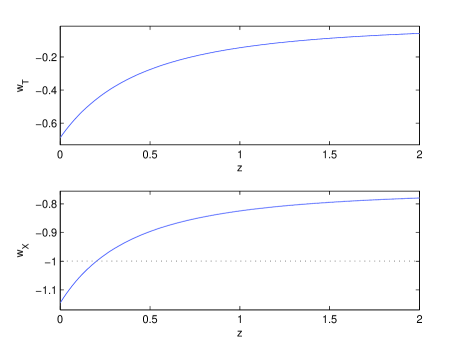
In Fig.1, we show the evolutions of the equation-of-state parameter for the total cosmological fluid $w_{T}$ and that for the effective dark fluid. Clearly, $w_{X}$ (down panel) cross the cosmological constant divide $w_{\Lambda}=-1$ recently, whereas $w_{T}$ is always greater than $-1$ (up panel) up to now. However, we note that both $w_{T}$ and $w_{X}$ will be less than $<-1$ and trend to negative infinity with the expansion of the universe. Therefore, the universe will suffer from the fate of so-call ”big-rip” in the future [15]. Interestingly, $w_{X}$ is a negative constant in the original power-law Cardassian model [9]. Therefore, this can lead to discrepancies between exponential and power-law models.

2.2 Model II: a modified version of exponential Cardassian model

We now consider the following modified version of the original Cardassian model:

$$g(\rho)=(\rho+\rho_{card})\exp\left[\left(\frac{q\rho_{card}}{\rho+\rho_{card}}\right)^{n}\right],$$ (11)

where $\rho_{card}$ is a characteristic constant energy density and $q$ and $n$ are two dimensionless positive constants. Obviously, at early times, $\rho$ is much larger than the characteristic energy density $\rho_{card}$, $g(\rho)\rightarrow\rho$, i.e. Eq.(11) recovers the standard Friedmann equation. In terms of Eqs.(11) and (6), the current acceleration expansion of the universe requires that

$$\sigma_{0}\left[1-3n\left(\frac{q}{1+\sigma_{0}}\right)^{n}\right]<2,$$ (12)

where we define the dimensionless quantity $\sigma\equiv\rho/\rho_{card}=\rho_{0}/\rho_{card}(1+z)^{3}\equiv\sigma_{0}(1+z)^{3}$.According to the assumption that the universe is flat, there is a relationship between the four parameters $\Omega_{m,0}$, $\sigma_{0}$, $q$ and $n$ that

$$(1+\sigma_{0})\exp\left[\left(\frac{q}{1+\sigma_{0}}\right)^{n}\right]=\sigma_{0}\Omega_{m,0}^{-1}.$$ (13)

Using the dynamics of $\rho$ and Eq.(13), the function $f_{X}(Z)$ in Eq.(7) that describe the evolution of the effective dark fluid becomes

$$f_{X}(z) = \frac{\Omega_{m,0}}{1-\Omega_{m,0}}\left\{\left[\sigma_{0}^{-1}+(1+z)^{3}\right]\exp\left[\frac{-(1+\sigma_{0})^{n}\ln[(1+\sigma_{0}^{-1})\Omega_{m,0}]}{\left[1+\sigma_{0}(1+z)^{3}\right]^{n}}\right]\right.$$ (14)

$$\hskip 56.9055pt\left.-(1+z)^{3}\right\}.$$

Combining Eqs.(14) and (13), it is easy to check that $f_{X}(z=0)=1$. Therefore, in this modified model, if we assume a priori value for $\Omega_{m,0}$ , there is only two free parameters $q$ and $n$ for the effective dark fluid as in the MP Cardassian model [11].

Using Eq.(6), we can get the effective parameter of equation of state $w_{T}$ for the total cosmological fluid in this model

$$w_{T}=-1+\frac{\sigma}{1+\sigma}\left[1+n\left(\frac{1+\sigma_{0}}{1+\sigma}\right)^{n}\ln[(1+\sigma_{0}^{-1})\Omega_{m,0}]\right],$$ (15)

and the equation-of-state parameter of effective dark fluid $w_{X}$ becomes

$$w_{X}=\frac{-1+{\sigma}n\left(\frac{1+\sigma_{0}}{1+\sigma}\right)^{n}\ln[(1+\sigma_{0}^{-1})\Omega_{m,0}]}{1+\sigma\left[1-\exp\left(\left(\frac{1+\sigma_{0}}{1+\sigma}\right)^{n}\ln[(1+\sigma_{0}^{-1})\Omega_{m,0}]\right)\right]}.$$ (16)

In the limit of $\sigma\rightarrow 0$, both $w_{T}$ and $w_{X}$ trend to $-1$, therefore, the expansion of the universe will speedup forever and in the end the universe becomes de-Sitter universe asymptotically. For the current epoch $\sigma(z=0)=\sigma_{0}$, therefore, the current value of $w_{X}$ is determined by

$$w_{X}(z=0)=\frac{-1+n\sigma_{0}\ln[(1+\sigma_{0}^{-1})\Omega_{m,0}]}{(1+\sigma_{0})(1-\Omega_{m,0})}.$$ (17)

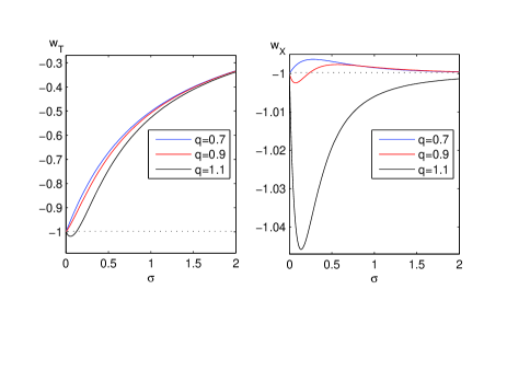
Obviously, the value of $w_{X}(z=0)$ can be greater or less than $-1$. Furthermore, from Fig.2, we can see the evolution of the $w_{X}(z)$. It is interesting that, for some values of parameters, $w_{X}$ can cross the cosmological constant divide $w_{\Lambda}=-1$ at a time.

Figure 2: The equation-of-state parameters $w_{T}$ and $w_{X}$ as two functions of $\sigma$ in the modified version of exponential Cardassian model for different values of parameter $q$, where we have chosen $\Omega_{m,0}=0.30$, $n=5$.

3 Fit the model parameters to Supernovae data

The Exponential Cardassian models predict a specific form of the Hubble parameter $H(z)$ as a function of redshift $z$ in terms of two parameters $\Omega_{m,0}$ and $n$. Using the relation between $d_{L}(z)$ and the comoving distance $r(z)$ (where $z$ is the redshift of light emission)

$$d_{L}(z)=r(z)(1+z),$$ (18)

and the light ray geodesic equation in a flat universe $c\;dt=a(z)\;dr(z)$ where $a(z)$ is the scale factor.

In general, the approach towards determining the expansion history $H(z)$ is to assume an arbitrary ansatz for $H(z)$ which is not necessarily physically motivated but is specially designed to give a good fit to the data for $d_{L}(z)$. Given a particular cosmological model for $H(z;a_{1},...,a_{n})$ where $a_{1},...,a_{n}$ are model parameters, the maximum likelihood technique can be used to determine the best fit values of parameters as well as the goodness of the fit of the model to the data. The technique can be summarized as follows: The observational data consist of $N$ apparent magnitudes $m_{i}(z_{i})$ and redshifts $z_{i}$ with their corresponding errors $\sigma_{m_{i}}$ and $\sigma_{z_{i}}$. These errors are assumed to be gaussian and uncorrelated. Each apparent magnitude $m_{i}$ is related to the corresponding luminosity distance $d_{L}$ by

$$m(z)=M+5\;\log_{10}\left[{{d_{L}(z)}\over{\mbox{Mpc}}}\right]+25,$$ (19)

where $M$ is the absolute magnitude. For the distant SNeIa, one can directly observe their apparent magnitude m and redshift z, because the absolute magnitude $M$ of them is assumed to be constant,i.e. , the supernovae are standard candles. Obviously, the luminosity distance $d_{L}(z)$ is the ‘meeting point’ between the observed apparent magnitude $m(z)$ and the theoretical prediction $H(z)$. Usually, one define distance modulus $\mu(z)\equiv m(z)-M$ and express it in terms of the dimensionless ‘Hubble-constant free’ luminosity distance $D_{L}$ defined by$D_{L}(z)={{H_{0}d_{L}(z)}/c}$ as

$$\mu(z)=5\;\log_{10}(D_{L}(z))+\mu_{0},$$ (20)

where the zero offset $\mu_{0}$ depends on $H_{0}$ (or $h$) as

$$\mu_{0}=5\;\log_{10}\left({{cH_{0}^{-1}}\over{\mbox{Mpc}}}\right)+25=-5\log_{10}h+42.38.$$ (21)

The theoretically predicted value $D_{L}^{th}(z)$ in the context of a given model $H(z;a_{1},...,a_{n})$ can be described by [16, 17, 18]

$$D_{L}^{th}(z)=(1+z)\int_{0}^{z}dz^{\prime}\;{{H_{0}}\over{H(z^{\prime};a_{1},...a_{n})}}.$$ (22)

Therefore, the best fit values for the parameters ($\Omega_{m,0},n$) of model I are found by minimizing the quantity

$$\chi^{2}(\Omega_{m,0},n)=\sum_{i=1}^{N}\frac{\left[\mu^{{obs}}(z_{i})-5\log_{10}D_{L}^{{th}}(z_{i};\Omega_{m,0},n)-\mu_{0}\right]^{2}}{\sigma_{i}^{2}}.$$ (23)

Since the nuisance parameter $\mu_{0}$ is model-independent, its value from a specific good fit can be used as consistency test of the data [19] and one can choose a priori value of it (equivalently, the value of dimensionless Hubble parameter $h$) or marginalize over it thus obtaining

$$\widetilde{\chi}^{2}(\Omega_{m,0},n)=A(\Omega_{m,0},n)-\frac{B(\Omega_{m,0},n)^{2}}{C}+\ln\left(\frac{C}{2\pi}\right),$$ (24)

where

$$A(\Omega_{m,0},n)=\sum_{i=1}^{N}\frac{\left[\mu^{{obs}}(z_{i})-5\log_{10}D_{L}^{{th}}(z_{i};\Omega_{m,0},n)\right]^{2}}{\sigma_{i}^{2}},$$ (25)

$$B(\Omega_{m,0},n)=\sum_{i=1}^{N}\frac{\left[\mu^{{obs}}(z_{i})-5\log_{10}D_{L}^{{th}}(z_{i};\Omega_{m,0},n)\right]}{\sigma_{i}^{2}},$$ (26)

and

$$C=\sum_{i=1}^{N}\frac{1}{\sigma_{i}^{2}}.$$ (27)

In the latter approach, instead of minimizing ${\chi}^{2}(\Omega_{m,0},n)$, one can minimize $\widetilde{\chi}^{2}(\Omega_{m,0},n)$ which is independent of $\mu_{0}$.

We now apply the above described maximum likelihood method using Gold dataset which is one of the reliable published data set consisting of 157 SNeIa ($N=157$) [2].

In Fig. 3, we show a comparison of the observed 157 SNeIa distance moduli along with the theoretically predicted curves in model I (continuous line). It is obvious that the exponential Cardassian model provide a good fit to the observational data.

Figure 3: The observed 157 Gold SNeIa distance modulus along with the theoretically predicted curves in model I (solid line), where we take a priori that current dimensionless Hubble parameter $h=0.65$.

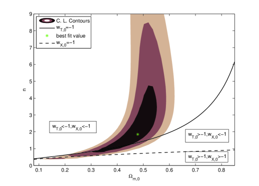
In Fig.4, contours with 68.3%, 95.4% and 99.7% confidence level are plotted, in which we take a marginalization over the model-independent parameter $\mu_{0}$. The best fit as showed in the figure corresponds to $\Omega_{m,0}=0.48$ and $n=1.84$, and the minimum value of $\chi^{2}=173.51$. Clearly, the allowed ranges of the parameters $\Omega_{m,0}$ and $n$ favor that there exists an effective phantom energy in the universe.

Figure 4: The 68.3%, 95.4% and 99.7% confidence contours of parameters $\Omega_{m,0}$ and $n$ using the Gold SNeIa dataset and marginalizing over the model-independent parameter $\mu_{0}$.

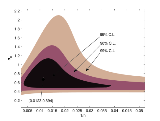
As for model II, using the above marginalization method, we find the minimum value of $\chi^{2}(\Omega_{m,0},\sigma_{0},n)$ is $173.08$ and the corresponding best-fit value of parameters are $\Omega_{m,0}=0.308$, $\sigma_{0}=0.708$ and $1/n=0.0142$. If we assume prior that $\Omega_{m,0}=0.3$ as indicated by the observation about mass function of galaxies, the minimum value of $\chi^{2}(\sigma_{0},n)$ is $173.178$ corresponding to $\sigma_{0}=0.694$ and $n^{-1}=0.0123$.

Figure 5: The 68%, 90% and 99% confidence level contours of parameters $\Omega_{m,0}$ and $n$ using the Gold SNeIa dataset and marginalizing over the model-independent parameter $\mu_{0}$ with a prior $\Omega_{m,0}=0.3$.

4 On the sound speed $c_{s}^{2}$

In order to guarantee the classical solution of the expansion is stable, the sound speed $c_{s}^{2}$ of classical perturbations of the total cosmological fluid around homogeneous FRW solutions should always be greater than zero. If the expansion of the universe is adiabatic, the sound speed of total cosmological fluid can be represented by $c_{s}^{2}=\delta p_{T}/\delta\rho_{T}$. For model I,

$$c_{s}^{2}=-n\ln(\Omega_{m,0}^{-1})(1+z)^{-3n}\frac{n\ln(\Omega_{m,0}^{-1})(1+z)^{-3n}+n-1}{n\ln(\Omega_{m,0}^{-1})(1+z)^{-3n}-1}.$$ (28)

In order to assure that $c_{s}^{2}>0$ at any time, we should have

$$n\ln(\Omega_{m,0}^{-1})(1+z)^{-3n}+n-1>0$$ (29)

and

$$n\ln(\Omega_{m,0}^{-1})(1+z)^{-3n}-1<0.$$ (30)

From condition (29), $n$ should be greater than $1$; but condition (30) can not be satisfied for every value of $z\in(-1,+\infty)$. Therefore, model I should only be considered as an effective description for the cosmic expansion. However, we note that if we only require that $c_{s}^{2}>0$ for $z>0$, i.e. , classical solution of the expansion is stable in the past, then we should let $-1<w_{T,0}<n-1$ which is clearly satisfiable.

As for model II, the sound speed can be denoted as

$$c_{s}^{2}=-\frac{n\sigma}{q}\left(\frac{q}{1+\sigma}\right)^{n+1}\frac{n\left(\frac{q}{1+\sigma}\right)^{n}+n-1}{n\left(\frac{q}{1+\sigma}\right)^{n}-1}.$$ (31)

It is easy to find that $c_{s}^{2}$ is always positive if the parameters satisfy the condition $q^{n}<n^{-1}<1$.

5 Discussion

In above sections, we have investigated a new kind of Cardassian models of the universe,dubbed Exponential Cardassian universe. Contrary to the original power-law Cardassian model [9], the equation-of-state parameter $w$ of effective dark fluid is dependent on time that can cross the cosmological constat divide $w_{\Lambda}=-1$ from $w_{X}>-1$ to $w_{X}<-1$ as the observations mildly indicate.

However, it is worth noting that these two models are available at much large scales where the matter density $\rho_{m}\sim\rho_{c}$ and evolve in the light of $\propto(1+z)^{-3}$. As discussed by Gondolo and Freese [14], the gradient of the effective Cardassian pressure $\nabla p_{card}$ should be able to neglected compared to that of the ordinary pressure $\nabla p_{m}$ at the scales of galaxies and galaxy clusters where the matter density is much larger than cosmic average density. In a typical galaxy where $\rho_{m}\sim 100\rho_{c}\sim 100\rho_{card}$ and $p_{m}=\rho_{m}\Sigma^{2}$ with velocity dispersion $\Sigma=300\;\mbox{km/s}$, if we assume that $\nabla p_{card}\ll\nabla p_{m}$, we should require the parameter $n$ in both models considered above are greater than $3$. It is remarkable that this value of $n$ is compatible with the data of SNeIa observations. Therefore, these two models are both available on galactic scales.

Observationally, the exponential Cardassian models are compatible with the data of SNeIa. The further work that should do is to check it out by other cosmological and astrophysical observations such as CMB and large scale structures (LSS) as many works (for example, [20, 21]) for power-law Cardassian models, which is out of the scope of this paper. However, it is worth noting that Koivisto et al [20] pointed out that in the MP Cardassian model, the late integrated Sachs-Wolf effect is typically very large duo to the suppression of fluctuations in Cardassian fluid at late times, and is then not compatible with the observations of CMB unless the parameters is very close to the $\Lambda$CDM model. In the exponential Cardassian models, we assume that Cardassian fluctuations is induced by cold dark matter (i.e., case III in Ref. [20]) and fluctuations in the cold dark matter and in the Cardassian fluid are related adiabatically

$$\delta=\left(\frac{d\log\rho_{T}}{d\log\rho}\right)^{-1}\delta_{T}=\frac{\delta_{T}}{1+w_{T}},$$ (32)

where $\delta$ and $\delta_{T}$ denote the fluctuations in cold dark matter and Cardassian fluid, respectively. According to the expressions of $w_{T}$, Eq.(9) for model I and Eq. (15) for model II, it is not hard to find that the Cardassian fluctuations are both not heavily suppressed as those in MP Cardassian model which $\delta\sim a^{3q}\delta_{T}$ at late times [20]. Therefore, in the exponential Cardassian models the above problem is alleviated to some extent.

Theoretically, these models, in fact as well as power-law Cardassian models, are phenomenologically described in a fluid approach, therefore, we need further works to find a simple fundamental theory which can derive the form of $g(\rho)$ presented above.

References

- [1] A. Riess et al., Astron. J. 116, (1998) 1009; S. J. Perlmutter et al., Astroph. J. 517, (1999) 565; J. L. Tonry et al., Astroph. J. 594, (2003) 1; B. Barris et al., Astroph. J. 602, (2004) 571; R. Knop et al., Astroph. J. 598, (2003) 102.
- [2] A. G. Riess et al.[Supernova Search Team Collaboration], Astrophys. J. 607, (2004) 665.
- [3] P. Astier et al., arXiv:astro-ph/0510447.
- [4] D. N. Spergel et al.[WMAP Collaboration], Astrophys. J. Suppl. 148, (2003) 175.
- [5] M. Tegmark et al.[SDSS Collaboration], Phys. Rev. D69, (2004) 103501 .
- [6] B. Ratra and P.J.E. Peebles, Rev. Mod. Phys. 75, (2003) 559; T. Padmanabhan, Phys. Rept. 380, (2005) 235; V. Sahni, astro-ph/0403324 and references therein.
- [7] P.J.E. Peebles and B. Ratra, Astrophys. J. 325, (1988) L17; P. J. Steinhardt, L. Wang and I. Zlatev, Phys. Rev. D59, (1999) 123504; X. Z. Li, J. G. Hao and D. J. Liu, Class. Quantum Grav., 19, (2002) 6049; D. J. Liu and X. Z. Li, Phys. Lett. B611, (2005) 8; X. Z. Li, J. G. Hao, D. J. Liu and X. H. Zhai, Int. J. Mod. Phys., A18, (2003) 5921.
- [8] R. R. Caldwell, Phys. Lett. B545, (2002) 23; J. G. Hao and X. Z. Li, Phys. Rev. D67, (2003) 107303; D. J. Liu and X. Z. Li, Phys. Rev. D68, (2003) 067301; J. G. Hao and X. Z. Li, Phys. Rev. D68, (2003) 043501; X. Z. Li and J. G. Hao, Phys. Rev. D69, (2004) 107303; J. G. Hao and X. Z. Li, Phys. Lett. B606, (2005) 7;G. Calcagni, hep-ph/0503044. S.Nojiri and S D Odintsov, Phys. Rev. D72,(2005) 023003; P.F. Gonzalez-Diaz, Phys. Lett. B586,(2004) 1.
- [9] K. Freese and M. Lewis, Phys. Lett. B540, (2002) 1.
- [10] K. Freese, New Astron. Rev. 49 (2005) 103; R. Lazkoz and G. Len, Phys. Rev. D71, (2005) 123516.
- [11] Y. Wang, K. Freese, P. Gondolo and M. Lewis, Astrophys. J. 594, (2003) 25.
- [12] C.B Netterfield et al., Astrophys. J. 571, (2002) 604; R. Stompor et al., Astrophys. J. Lett. 561, (2001) L7; N.W Halverson et al., Astrophys. J. 568, (2002) 38.
- [13] A. Melchiorri, L. Mersini, C. Odman, and M. Trodden, Phys. Rev. D68, (2003) 043509; D. Huterer and A. Cooray, Phys. Rev. D71, (2005) 023506.
- [14] P. Gondolo, K. Freese Phys.Rev. D68 (2003) 063509.
- [15] R.R. Caldwell, M. Kamionkowski and N.N. Weinberg, Phys. Rev. Lett. 91 (2003) 071301; J. G. Hao and X. Z. Li, Phys. Rev. D70, (2004) 043529; Phys. Rev. D72,(2005) 043527.
- [16] A. A. Starobinsky, JETP Lett. 68, (1998) 757.
- [17] D. Huterer and M. S. Turner, Phys. Rev. D64, (2001) 123527.
- [18] T. Chiba, N. Sugiyama and T. Nakamura, Mon. Not. Roy. Astron. Soc. 301, (1998) 72.
- [19] T. R. Choudhury and T. Padmanabhan, Astron. Astrophys. 429, (2005) 807.
- [20] T. Koivisto, H. Kurki-Suonio and F. Ravndal, Phys.Rev. D71, (2005) 064027.
- [21] M. Amarzguioui, O. Elgaroy and T. Multamaki, JCAP 0501, (2005) 008;