Determination of the Cosmic Distance Scale from
Sunyaev-Zel’dovich Effect and Chandra X-ray
Measurements of High Redshift Galaxy Clusters
Abstract
We determine the distance to 38 clusters of galaxies in the redshift range 0.14z0.89 using X-ray data from Chandra and Sunyaev-Zeldovich Effect data from the Owens Valley Radio Observatory and the Berkeley-Illinois-Maryland Association interferometric arrays. The cluster plasma and dark matter distributions are analyzed using a hydrostatic equilibrium model that accounts for radial variations in density, temperature and abundance, and the statistical and systematic errors of this method are quantified. The analysis is performed via a Markov chain Monte Carlo technique that provides simultaneous estimation of all model parameters. We measure a Hubble constant of km s-1 Mpc-1(statistical followed by systematic uncertainty at 68% confidence) for an , =0.7 cosmology. We also analyze the data using an isothermal model that does not invoke the hydrostatic equilibrium assumption, and find km s-1 Mpc-1; to avoid effects from cool cores in clusters, we repeated this analysis excluding the central 100 kpc from the X-ray data, and find km s-1 Mpc-1 (statistical followed by systematic uncertainty at 68% confidence). The consistency between the models illustrates the relative insensitivity of SZE/X-ray determinations of to the details of the cluster model. Our determination of the Hubble parameter in the distant universe agrees with the recent measurement from the Hubble Space Telescope key project that probes the nearby universe.
1 Introduction
Combined analysis of radio and X-ray data provides a method to determine directly the distances to galaxy clusters. Galaxy clusters are the largest gravitationally collapsed structures in the universe, with a hot diffuse plasma ( K) that fills the intergalactic space. Cosmic microwave background (CMB) photons passing through this hot intracluster medium (ICM) have a % chance of inverse Compton scattering off the energetic electrons, causing a small ( mK) distortion of the CMB spectrum, known as the Sunyaev-Zel’dovich Effect (SZE: Sunyaev & Zel’dovich 1970, 1972; for reviews see Birkinshaw 1999; Carlstrom, Holder, & Reese 2002). The same hot gas emits X-rays primarily through thermal bremsstrahlung. The SZE is a function of the integrated pressure, , where and are the electron number density and temperature of the hot gas, and the integration is along the line-of-sight. The X-ray emission scales as , where is the X-ray cooling function. The different dependences on density, along with a model of the cluster gas, enable a direct distance determination to the galaxy cluster. This method is independent of the extragalactic distance ladder and provides distances to high redshift galaxy clusters.
The mK SZE signal proved challenging for initial searches, but recent improvements in both technology and observational strategies have made observations of the SZE fairly routine. High signal-to-noise ratio (S/N) detections of the SZE have been made with single dish observations at radio wavelengths (Birkinshaw and Hughes 1994; Herbig et al. 1995; Myers et al. 1997; Hughes and Birkinshaw 1998; Mason et al. 2001), millimeter wavelengths (Holzapfel et al. 1997a,b; Pointecouteau et al. 1999, 2001) and submillimeter wavelengths (Lamarre et al. 1998; Komatsu et al. 1999), while interferometric observations at centimeter wavelengths have produced images of the SZE (Jones et al. 1993; Grainge et al. 1993; Carlstrom et al. 1996, 2000; Grainge et al. 2002; Reese et al. 2000, 2002; Grego et al. 2000, 2001; La Roque et al. 2003; Udomprasert et al. 2004).
SZE/X-ray distances provide a measure of the Hubble constant that is independent of the extragalactic distance ladder and probe high redshifts, well into the Hubble flow. The SZE/X-ray determinations of bridge the gap between observations of nearby objects (e.g. the Hubble Space Telescope Key Project, Freedman et al. 2001) and expansion values inferred from CMB anisotropy (Spergel et al. 2003) and supernova (Riess et al. 2005) measurements. Previous SZE/X-ray determinations of the Hubble parameter have progressed from analysis of individual galaxy clusters, to samples of a few (Myers et al. 1997; Mason et al. 2001; Jones et al. 2005), up to a sample of 18 galaxy clusters using ROSAT X-ray data (Reese et al 2002; for reviews see Reese 2004 and Carlstrom, Holder, & Reese 2002). In most cases, simple isothermal models were adopted for the cluster gas, since the data did not warrant a more sophisticated treatment.
We present a Markov chain Monte Carlo joint analysis of interferometric SZE observations and Chandra X-ray imaging spectroscopy observations of a sample of 38 galaxy clusters with redshifts . The unprecedented spatial resolution of Chandra combined with its simultaneous spectral resolution allow more realistic modeling of the intracluster plasma than previous studies, thus enabling a more accurate determination of the Hubble constant.
2 Observations of galaxy clusters
2.1 Interferometric Sunyaev-Zel’dovich effect data
Interferometric radio observations of the 38 clusters in Table 1 were performed at the Berkeley-Illinois-Maryland Association observatory (BIMA) and at the Owens Valley Radio Observatory (OVRO). The arrays were equipped with 26-36 GHz receivers to obtain maps of the Sunyaev-Zel’dovich Effect (SZE) toward the clusters (Carlstrom et al. 1996, 2000; Reese et al. 2000). These frequencies are on the Rayleigh-Jeans end of the microwave spectrum, and the scattering with cluster electrons causes an intensity decrease that, in terms of brightness temperature, corresponds to a change in of order mK.
Most of the OVRO and BIMA telescopes were placed in a compact configuration to maximize the sensitivity on angular scales subtended by distant clusters (typically ) and a few telescopes were placed at longer baselines for simultaneous point source imaging (Reese et al. 2002). The SZE data consist of the position in the Fourier domain (- plane) and the visibilities — the real and imaginary Fourier component pairs as functions of and , which are the Fourier conjugate variables to right ascension and declination. The effective resolution of the interferometer, the synthesized beam, depends on the - coverage and is therefore a function of the array configuration and source position. A typical size for the synthesized beam of our observations is , as shown in Figure 1. The SZE data were reduced using the MIRIAD (Sault et al. 1995) and MMA (Scoville et al. 1993) software packages and images were made with DIFMAP (Pearson et al. 1994) software. Absolute flux calibration was peformed using Mars observations adopting the brightness temperature from the Rudy (1987) Mars model. The gain was monitored with observations of phase calibrators, and remained stable at the 1% level over a period of months. Data were excised when one telescope was shadowed by another, when cluster observations were not bracketed by two phase calibrators, when there were anomalous changes in the instrumental response between calibrator observations, or when there was spurious correlation. Positions of point sources were identified using the long baseline data; their fluxes are included as free parameters in the model, using the same methodology as Reese et al. (2002). Additional details of the SZE data analysis are provided in Reese et al. (2002) and Grego et al. (2000).
2.2 Chandra X-ray data
The Chandra X-ray data for the 38 clusters in our sample were obtained primarily through the Guaranteed Time program of Leon van Speybroeck. The observations were performed with the ACIS-I and ACIS-S detectors. The two ACIS instruments provide spatially resolved X-ray spectroscopy and imaging with an angular resolution of and with energy resolution of eV. Data analysis was performed with the CIAO software (version 3.2) and the CALDB calibration information (version 3.1) provided by the Chandra calibration team (Chandra Interactive Analysis of Observations, http://cxc.harvard.edu/ciao/).
The first step in the data analysis was to process the Level 1 data to correct for the charge transfer inefficiency of the ACIS detectors. We then generated a Level 2 event file applying standard filtering techniques: we selected grade=0,2,3,4,6, status=0 events (as defined in the Chandra Proposers Observatory Guide) and filtered the event file for periods of poor aspect solution using the good time interval (GTI) data provided with the observations. Periods of high background count rates were occasionally present, typically due to Solar flares (Markevitch 2001). We discarded these periods using an iterative procedure in which we constructed a light-curve of a background region in 500 second bins, and time intervals that were in excess of the median count rate by more than 3 were discarded from the dataset. The Chandra instruments are affected by the buildup of a contaminant on the optical blocking filter located along the optical path to the ACIS detector; we accounted for this efficiency reduction using CIAO and CALDB. Spectra were accumulated in concentric annuli centered at the peak of the X-ray emission, each containing approximately the same number of source photons after removal of point sources. Both images and spectra were limited to 0.7-7 keV in order to exclude the low-energy and high-energy data that are more strongly affected by background and by calibration uncertainties. The X-ray images were binned in 1.97′′ pixels; this sets the limiting angular resolution of our X-ray data, as the Chandra/ point response function in the center of the X-ray image is smaller than our adopted pixel size. The X-ray background was measured for each cluster exposure, using peripheral regions of the detector (ACIS-S) or adjacent detector chips (ACIS-I) that are source free. Additional details of the Chandra X-ray data analysis are provided in Section 2 of Bonamente et al. (2004).
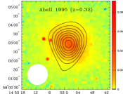
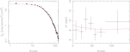
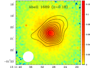
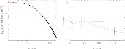
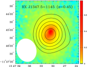
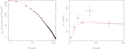
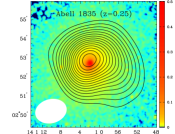
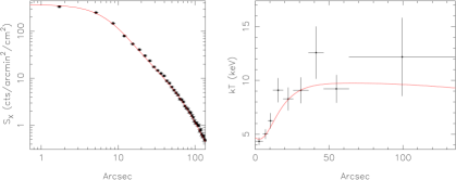
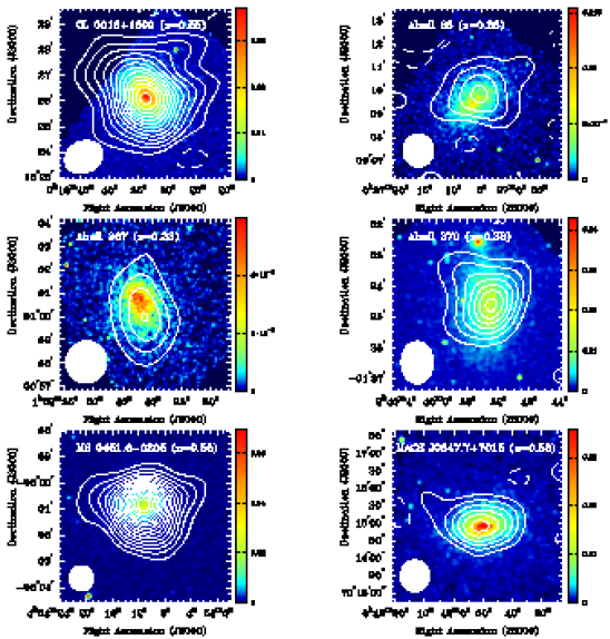
Images of the X-ray surface brightness of selected clusters are shown in Figure 1, with SZE contours overlaid, and in Appendix 1 for all 38 clusters. Chandra also provides spatially-resolved spectroscopy that allows a determination of the temperature and metal abundance of the hot plasma. The spectral properties of the plasma are obtained by fits to an optically thin emission model, with absorbing column fixed at the Galactic value. The uncertainty in of cm-2 (Dickey and Lockman 1990) results in uncertainties in the measured temperatures of less than 1%, and therefore has a negligible effect in the measurement of the cluster distances. In Figure 1 we show the radial profiles of the X-ray surface brightness and of the plasma temperature for several representative clusters, along with their best fit curves as determined from the modeling described in the next Section; radial brightness and temperature profiles for the full cluster sample are presented in Appendix 2 and 3.
In Figure 2 we show the composite radial temperature profiles for the 38 clusters. The clusters containing plasma with a central cooling time , which we refer to as the“cool core” sample, are shown on top, while clusters with longer cooling times are shown on the bottom 111The clusters with are Abell 586, MACS J0744.8+3927, ZW 3146, Abell 1413, MACS J1311.0-0310, Abell 1689, RX J1347.5-1145, MS 1358.4+6245, Abell 1835, MACS J1423.8+2404, RX J2129.7+0005, Abell 2163, Abell 2204 and Abell 2261. The Hubble time is approximately (Carroll, Press and Turner 1992) with =72 km s-1 Mpc-1 and the cooling time () is calculated using the central density and the temperature from an isothermal model fit. . The temperature profiles for the 38 clusters lie within the envelope of the 21 clusters observed by BeppoSAX (see Fig. 3, Fig. 4 and Table 2 of De Grandi and Molendi 2002). The spectra were extracted in concentric annuli that contain a similar number of photons in each annulus for each cluster. The radial temperature profile data for all clusters, including the temperature, the background-subtracted counts and the , are reported in Appendix 3 (Table 7). Metal abundances of the hot cluster plasma have a marginal effect on the X-ray cooling function (see Section 3). We assume the De Grandi et al. (2004) abundance profile in our analysis, which is consistent with our measured abundances.


3 Measuring distances with X-ray and Sunyaev-Zel’dovich Effect data
3.1 The hydrostatic equilibrium model
To determine the distance to a cluster, we must first construct a realistic model for the cluster gas distribution. At the center of clusters the density may be high enough that the radiative cooling time-scale is less than the cluster’s age, leading to a reduction in temperature and an increase in central density. This increases the central X-ray emissivity in the Chandra passband, as shown in Figure 1 for the clusters RXJ 1347.5-1145 and Abell 1835. At large radii, the density of the gas is sufficiently low that X-ray emission can be sustained for cosmological periods without significant cooling. Cool core clusters effectively exhibit two components: a centrally concentrated gas peak and a broad, shallower distribution of the gas. This phenomenon motivates the modelling of the gas density with a function of the form:
| (1) |
This shape generalizes the single -model profile, introduced by Cavaliere and Fusco-Femiano (1976) and commonly used to fit X-ray surface brightness profiles, to a double -model of the density that has the freedom of following both the central spike in density and the more gentle outer distribution. A double -model of the surface brightness was first used by Mohr et al. (1999) to fit X-ray data of galaxy clusters; the density model of Equation 1 was further developed by La Roque (2005). The quantity is the central density, governs the fractional contributions of the narrow and broad components (), and are the two core radii that describe the shape of the inner and outer portions of the density distribution and determines the slope at large radii (the same is used for both the central and outer distribution in order to reduce the total number of degrees of freedom).
The X-ray surface brightness is related to the gas density as
| (2) |
where is the cluster redshift, is the electron density of the plasma (Equation 1), is the X-ray cooling function, and the integration is performed along the line of sight . We calculate as a function of plasma temperature and energy in the rest frame of the cluster, including contributions from relativistic electron-ion thermal bremsstrahlung, electron-electron thermal bremsstrahlung, recombination, and two photon processes; the cooling function is then redshifted to the detector frame, convolved with the telescope and detector response, and integrated over the 0.7-7 keV Chandra bandpass, following the method described in Reese et al. (2000). The calculation of requires a temperature profile in order to perform the integration, which we determine from our Chandra data (Figure 2). The appropriate response for each image was generated from CIAO.
The SZE decrement is proportional to the integrated gas pressure as
| (3) |
where is the frequency dependence of the SZE, and at our observing frequency of 30 GHz, K (Fixsen et al. 1996), is the Thomson cross section, is the Boltzmann constant, is the speed of light in vacuum, is the electron mass, the electron temperature, and the integration is along the line of sight.
Historically, the cluster distance has been solved for directly by taking advantage of the different density dependences of the X-ray emission and SZE decrement (e.g., Hughes, Birkinshaw and Arnaud 1991; Reese et al. 2002; Bonamente et al. 2004):
| (4) | |||
The details of the plasma modelling, such as the numerical integration of the density profile, are included in the proportionality constants of Equations 4. The cluster angular diameter distance , where is the line-of-sight angular size, can be inferred with a joint analysis of SZE and X-ray data by assuming a cluster geometry to relate the measured angular size in the plane of the sky to that along the line of sight. For our adopted spherical geometry, these two sizes are equal.
Our model includes the distribution of dark matter in clusters. The baryonic matter reaches hydrostatic equilibrium in the potential well defined by the baryonic and dark matter components, on a time scale that is shorter than the cluster’s age (Sarazin 1988). Under spherical symmetry, this results in the condition
| (5) |
where is the gas pressure, is the gas density and is the gravitational potential due to both dark matter and the plasma. Using the ideal gas equation of state for the diffuse cluster plasma, where is the mean molecular weight and is the proton mass, one obtains a relationship between the cluster temperature and the cluster mass distribution:
| (6) |
We combine these hydrostatic equilibrium equations with a dark matter density distribution from Navarro, Frenk and White (1997):
| (7) |
where is a density normalization constant and is a scale radius. These model equations are combined with the X-ray and SZE data using a Markov chain Monte Carlo method, described in the following Section.
In Figure 1 the best-fit line (in red) of the X-ray surface brightness is obtained using the density distribution of Equation 1 and the hydrostatic equilibrium model described in this Section. For clusters in which a single model is an acceptable fit to the X-ray surface brightness (1.5; see Appendix 2), we simplify the density model of Equation 1 by fixing the parameter . We fit spherically symmetric models to all of the clusters, including those which do not appear circular in X-ray and radio observations, as this approach gives an unbiased estimator of cluster distances when a large sample of clusters is used (Sulkanen 1999).
3.2 Parameter estimation using the Markov chain Monte Carlo method
Our model consists of five parameters that describe the gas density (, , , and ; Equation 1), two parameters that describe the dark matter density ( and from Equation 7) and the angular diameter distance . Additional parameters such as the cluster position, point source positions, and point source fluxes are also included. A detailed discussion of radio point sources is provided in Reese et al. (2002). By linking the central densities between the X-ray and SZE datasets, and allowing to vary, the model can be integrated along the line of sight and compared with the X-ray and SZE data simultaneously, according to Equations 2 and 3. The model parameters can also be used with Equation 6 to solve for the cluster temperature profile, which is integrated along the line of sight and compared with the spectral data as described below. The Markov chain Monte Carlo (MCMC) method used to estimate the model parameters is described in Bonamente et al. (2004). In this Section we provide a brief overview of the method, focusing on the changes we applied to accommodate the new hydrostatic equilibrium model of Section 3.1.
The first step of the Markov chain Monte Carlo method is the calculation of the joint likelihood of the X-ray and SZE data with the model. This calculation follows three independent steps, one for each of the datasets involved: SZE data, X-ray images, and X-ray spectra. The likelihood calculation for the SZE data is performed directly in the Fourier plane, where the data are taken and where we understand the noise properties of the data. The likelihood is given by
| (8) |
where and are the difference between model and data for the real and imaginary components at each point in the Fourier plane, and is a measure of the Gaussian noise ().
Since the X-ray counts are distributed according to Poisson statistics, the likelihood is given by
| (9) |
where is model prediction (including cluster and background components), and is the number of counts detected in pixel . For details on the X-ray/SZE joint analysis, see Reese et al. (2000).
The spectral likelihood is calculated by comparing the predicted temperature profile with the observed one:
| (10) |
where labels the bins in the temperature profile (Figure 2), , and are the measured and model-predicted temperatures, and is the measured temperature uncertainty. The last term on the right in Equation 10 depends only on the data and will cancel when performing the likelihood ratio test. Likelihood evaluation for the spectral data requires another numerical integration to solve for , according to Equation 6. This temperature profile is weighted by the square of the density and the cooling function (Equation 2) and then integrated along the line of sight to determine the emission-weighted temperature profiles, which can be directly compared with the measured temperature profile. The joint likelihood of the spatial and spectral models is given by
.
A Markov chain is a sequence of model parameters constructed with the property that the model parameters appear in the chain with a frequency that is proportional to their posterior probability, i.e., the probability of occurrence in the light of the current observations. We start by assuming vague prior probability distributions for all parameters as top-hat functions between two extreme values. The first link of the MCMC is chosen as the midpoint of the prior distributions. We then select a candidate for the next link in the chain using a proposal distribution, in our case a simple top-hat function of constant width around the previous parameter values. These candidate parameter values are accepted into the chain or rejected according to the Metropolis-Hastings criterion (Metropolis 1953, Hastings 1970) that takes into account the likelihood information. This process is iterated for a large number of steps, which we chose as 100,000. This number ensures that the MCMC has reached convergence towards the posterior probability distribution functions of the parameters (Bonamente et al. 2004). Convergence is tested using the Raftery-Lewis test (Raftery and Lewis 1992; Gilks et al. 1996), the Gelman-Rubin test (Gelman and Rubin 1992) and the Geweke test (Geweke 1992). Confidence intervals for the model parameters are obtained by computing the cumulative distribution of the occurrence for each model parameter. We consider the median of the distribution as the best-fit value and calculate 68% confidence intervals around the median.
The results of the MCMC analysis are shown in Table 2, in which we report the best-fit values of , , , , , , and for each cluster.
3.3 Uncertainty analysis
The uncertainties in Table 2 represent the photon-counting statistical uncertainties of the X-ray images and spectra, and the statistical uncertainty of the SZE observations, as described in Section 3.2. Other sources of statistical and systematic uncertainty that affect our measurements are discussed in this Section and listed in Table 3. For comparison with the uncertainties encountered in previous studies, see Reese et al. (2002). We note that the Chandra and OVRO/BIMA sample allows us to obtain a distance scale measurement averaged over a large number of clusters; this ensemble average significantly reduces the impact of the single-cluster statistical uncertainies shown in Tables 2 and 3.
In the uncertainty analysis we make use of the following relationship that follows from Equation 4, as shown in Bonamente et al. (2004):
| (11) |
Note that is proportional to and (since ), so the distance determination is strongly dependent on the accuracy of the SZE decrement and X-ray temperature measurements.
3.3.1 Uncertainty in Galactic
In the spectral fits of Section 2.2 we used the HI column densities of Dickey and Lockman (1990), which have an uncertainty of = cm-2. A variation of the HI column density will primarily affect the best-fit X-ray temperature. The temperature, in turn, affects the measurement of cluster distances through Equation 11, , in which the X-ray cooling function is . We obtained spectral fits of our clusters using and as the HI column densities, and found that the best-fit temperatures change by less than 0.5%. The uncertainty in Galactic therefore results in a uncertainty of % ().
3.3.2 Cluster asphericity
Most clusters do not appear circular in X-ray or radio observations (e.g., Mohr et al. 1995). Numerical simulations by Sulkanen (1999) show that a spherical model fit to triaxial X-ray and SZE clusters yields an unbiased estimate of cluster distance when a large ensemble of clusters is used; the standard deviation of the measured distance for one cluster is %.
3.3.3 Small scale clumps in the intracluster gas
Clumping of the intracluster medium on scales smaller than the Chandra resolution is a potential source of systematic error. The presence of clumps enhances the measured X-ray emission () by the factor:
| (12) |
A factor C1 results in a measured angular diameter distance () that is lower than what one measures if no clumping is present, and such should be increased by a factor of if clumping occurs. In this case, the resulting best-fit would decrease.
Concurrent studies by LaRoque et al. (2006) suggest that as long as the clumps of X-ray emission observed by Chandra are excised from the data, the clusters in this sample are not affected by additional clumping of the hot gas. We therefore do not include this source of uncertainty in our error analysis. There is indication that clumpiness of the gas may be a factor for high-redshift clusters (Jeltema et al. 2005), and this effect may in principle lead to increased scatter at large z in Figure 3.
3.3.4 Point sources in the field
Undetected radio point sources near the cluster center mask the central decrement. According to Equation 11, , and an underestimate of the SZE decrement will result in an underestimate of the cluster distance. The synthesized beam of the SZE instrument also has negative sidelobes, and therefore overestimates of the decrement are also possible. A detailed treatment of the effect of point sources by La Roque et al. (2006) using this cluster sample result in a % uncertainty in the determination of .
For the X-ray data, the superior angular resolution of Chandra allows one to locate the point sources and mask them from the analysis, so no uncertainty from undetected X-ray point sources is introduced.
3.3.5 Kinetic SZE effect and CMB anisotropies
Peculiar velocities of clusters introduce a distortion in the CMB spectrum, known as the kinetic SZE. For a typical line-of-sight peculiar velocity of 300 km s-1 (Watkins 1997, Colberg et al. 2000) and a cluster of keV, the kinetic SZE is 4% of the thermal SZE. Since , the kinetic SZE effect introduces an uncertainty of 8% to the determination of cluster distances.
Limits on CMB anisotropies have been measured by Dawson et al. (2001, 2006) and Holzapfel et al. (2000) with BIMA at the frequency and angular scales of the observations presented in this paper. The 68% confidence upper limit is K at ( 2 ′scales). This results in a 68% uncertainty of 1% in the measurement of , and 2% in the measurement of . Both of these effects are expected to average out for a sample of clusters widely separated on the sky.
3.3.6 Radio halos and relics
Extended steep-spectrum nonthermal radio halo sources have been detected in the center of several clusters (Giovannini and Feretti 2000; Giovannini et al. 1999; Hanish 1982), and similar extended sources (radio relics) have also been found in other clusters at large radii from the cluster core (Giovannini and Feretti 2004; Feretti 2004). The on-center radio halo sources can mask the SZE decrement, resulting in an underestimate of . Reese et al. (2002) determined that the average effect of a radio halo at the BIMA and OVRO frequency is small: 1.5% of the thermal decrement. We include a one-sided +3% systematic uncertainty in the measurement to account for the possible presence of extended non-thermal radio halo emission in the cluster core. The frequency of occurrence and the flux of radio relic and radio halo sources are similar (Feretti 2004), but radio relics are attenuated by the interferometer due to their large displacement from the cluster center; we estimate that the systematic uncertainty due to radio relic sources is negligible (1%).
3.3.7 X-ray background
The X-ray background is measured following the method described in Section 2.2 and in Bonamente et al. (2004). For each cluster, we measure the 0.7-7 keV counts in a background region, with a statistical error equal to the square root of the number of counts, and extract a background spectrum from the same region. We assessed the effect of the X-ray background subtraction on the distance measurements by performing the following analysis. For the spatial analysis, we used the upper and lower limits of the measured background level; in the spectral analysis, we used the temperatures obtained by subtracting the background spectrum, rescaled by an amount equal to the fractional error of the measured background level. These additional MCMC runs resulted in measurements that are within 2% of those obtained with the nominal background. We therefore add a uncertainty in the measurement of .
3.3.8 X-ray calibration
The absolute calibration of the Chandra ACIS effective area is known to 5% in the 0.7-7 keV band of interest (http:/asc.harvard.edu/cal). This uncertainty affects the measurements directly through the surface brightness terms in Equation 11, resulting in a 5% systematic uncertainty on .
Temperature measurements with Chandra may be subject to systematic offsets caused by effective area and energy calibration errors, which we estimate at 5% (http:/asc.harvard.edu/cal). According to Equation 11, , where , therefore the effect of the temperature measurement uncertainty results in a 7.5% uncertainty on the distance for one cluster.
3.3.9 SZE calibration
The absolute calibration of the interferometric observations is known to about 4%, resulting in an uncertainty of 8% in the distance measurement of one cluster. Reese et al. (2002) also studied the effect of imprecisions in the measurement of the BIMA and OVRO primary beams, and conclude that the effect on distance measurements is negligible.
4 Measurement of the Hubble constant
We now use the 38 cluster distances to estimate the Hubble constant. The angular diameter distance is a function of the cluster redshift , the mass density , the dark energy density , and the Hubble constant , which is the overall normalization:
| (13) |
where the function is defined as for , for , for , and (Carroll, Press and Turner 1992)222Throughout this paper, , , and are defined at the present epoch (cf. Carroll, Press, and Turner 1992).. Observations of the CMB anisotropy (Spergel et al. 2003), high-redshift supernovae (Riess et al. 2004; Knop et al. 2003; Tonry et al. 2003) and mass measurements of galaxy clusters (e.g.,Grego et al. 2001; Vikhlinin et al. 2003; Allen et al. 2004) indicate a flat, dark energy-dominated universe with and , and these values are adopted in all subsequent analyses unless otherwise specified.
4.1 Measurement of the Hubble constant using the hydrostatic equilibrium model
We fit the theoretical function to our sample of 38 cluster distances obtained with the hydrostatic equilibrium model. For the fit, we combine the statistical errors given in Table 3 with the data modelling errors in Table 2, and obtain km s-1 Mpc-1(68% confidence interval, statistical uncertainty only). The fit uses the MCMC parameter estimation method described in section 3.2, with the likelihood calculated using Equation 10. The statistic of the best-fit model is 31.6 for 37 degrees of freedom.
The total systematic errors in are calculated by combining the individual systematic uncertainties of Table 3 in quadrature, applying the resulting errors to all 38 cluster distances, and repeating the fit. We obtain a systematic uncertainty in of (+10.0,-8.0) km s-1 Mpc -1.
Figure 3 shows the Chandra/SZE cluster distance measurements, and the theoretical curve for the best-fit Hubble constant =76.9 km s-1 Mpc-1 and , .
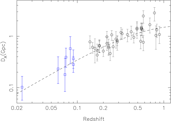
We also show the angular diameter distances of nearby clusters from Mason et al. (2001), to demonstrate that the best-fit curve is in agreement with low-redshift X-ray/SZE measurements. Our measurement of in the distant universe is in agreement with the Hubble Space Telescope Key Project measurement of km s-1 Mpc-1 (Freedman et al. 2001), which probes the nearby universe.
To address the effects of cosmology on the value of the Hubble constant obtained from the SZE/X-ray method, we also repeat the fit of our cluster distances varying the and in a fiducial interval around the currently favored CDM model parameters, and . The fits yield (68% statistical error), with a statistic for , =0.8, and () for , =0.6. Finally, we fit of our cluster distances with the theoretical function for a matter-dominated universe with and . The best-fit value of the Hubble constant in this case is =67.1 (68% statistical error), with a statistic of 32.5 for 37 degrees of freedom. These fits have the same quality as that for the currently favored , cosmology, indicating that cluster distances alone can not yet effectively constrain the energy density parameters.
4.2 Measurement of the Hubble constant using the isothermal -model
We compare the cluster distance results from the hydrostatic model of Section 4.1 to the results from other ICM models to determine how sensitive the distance measurements are to the details of the plasma modeling. These models consist of a simple isothermal -model, with a density profile described by Equation 1 with =0, and with a constant temperature. Since cluster centers often feature a sharp gradient in density and temperature, not consistent with this simple =0 model, we also excised the central kpc of the X-ray data from the analysis. Figure 2 and Table 7 show that, when the central 100 kpc are removed from the X-ray data, the temperature profiles out to 600 kpc are essentially flat. With these simplifying assumptions, the X-ray surface brightness and SZE decrement have simple analytical functions (see, e.g., Birkinshaw et al. 1991), and numerical integrations are no longer needed. Also, we do not enforce hydrostatic equilibrium, and accordingly do not consider the dark matter distribution and the spectral likelihood information in the MCMC procedure described in Section 3.2.
There is no simple way to mask the central 100 kpc from our interferometric data, because these data are fit in the Fourier plane (La Roque 2005). However, the SZE data are less sensitive to the presence of a dense core than the X-ray data (Equation 4), and the X-ray data drive the fit for the density shape parameters. In addition, even clusters with X-ray structures in the core are normally in pressure equilibrium (Markevitch et al. 2000, 2001), and should therefore have smooth SZE profiles. We therefore use the entire SZE dataset and the 100 kpc-cut X-ray dataset for this analysis. The assumptions of the model outlined above are described and tested in more detail in La Roque et al. (2006).
The model includes the following parameters: , , , , and , with the X-ray surface brightness and the SZE decrement following the equations
| (14) | |||
| (15) |
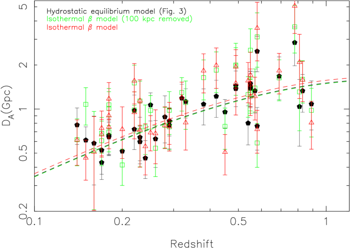
The angular diameter distance is calculated according to Equation 11, which is explained in detail in Bonamente et al. (2004). Applying this simple model to the data, we calculate the model parameters (Table 4) and the angular diameter distances (Figure 4). The same fitting technique employed in Section 4.1 above yields a best-fit Hubble constant of km s-1 Mpc-1(68% confidence interval, statistical followed by systematic errors), with a fit statistic of =53.9 for 37 degrees of freedom. In this joint X-ray/SZE analysis, the spatial parameters , , and are constrained almost exclusively by the X-ray data, rather than by the SZE imaging, due to the high angular resolution and the large number of counts in the Chandra/ images. Constraints on are obtained from the SZE data, while and are obtained from the X-ray spectroscopy. The value of performing the joint MCMC analysis involving all three datasets is that the full probability density function for each model parameter can be obtained, with all statistically-allowable parameter variations included.
Finally, we include the results for the standard isothermal model fit to the entire X-ray dataset, i.e., without the excision of the central 100 kpc. This exercise is provided for comparison with earlier analyses that used such modelling (e.g., Reese et al. 2002), and it is useful to assess the impact of the bright cluster cores on the determination of the distance scale. This model yields the best-fit parameters in Table 5, the angular diameter distances of Figure 4 and a best-fit Hubble constant of km s-1 Mpc-1(68% confidence interval, statistical followed by systematic errors), with a fit statistic of =53.1 for 37 degrees of freedom.
These results indicate that the measurement of the cosmic distance scale using X-ray and SZE observations of galaxy clusters is insensitive to the details of the hot ICM model: the spread between the three models explored here is 3 km s-1 Mpc-1.
4.3 Comparison with recent distance measurements
We compare our results with recent X-ray/SZE measurements of the Hubble constant using clusters in our sample.
Jones et al. (2005), Saunders et al. (2003) and Grainge et al. (2002) use ROSAT and ASCA X-ray data and SZE data from the Ryle telescope for Abell 697, Abell 773, Abell 1413, Abell 1914 and Abell 2218. They employ an ellipsoidal model to find km s-1 Mpc-1 for a CDM cosmology, in agreement with our hydrostatic equilibrium model and our isothermal model results.
Schmidt, Allen and Fabian (2004) use Chandra X-ray data and several published SZE measurements of RXJ1347.5-1145, Abell 1835 and Abell 478 (the latter not included in our sample), and employ a hydrostatic equilibrium model similar to the one used in this paper. They obtain a best-fit km s-1 Mpc-1 for a CDM cosmology, also in agreement with our hydrostatic equilibrium model results.
Worrall and Birkinshaw (2003) use a model fit to the XMM-Newton X-ray data and the Hughes and Birkinshaw (1998) SZE data of CL0016+1609 to find a best-fit Gpc. This measurement is in excellent agreement with our hydrostatic equilibrium model for this cluster ( Gpc, Table 2) and isothermal models ( Gpc, Table 4; Gpc, Table 5).
5 Conclusions
We analyzed 38 clusters of galaxies with Chandra X-ray imaging spectroscopy and OVRO-BIMA SZE data, the largest sample to date used to measure . We applied a hydrostatic equilibrium model that accounts for radial variations in cluster temperature, and for sharp density gradients caused by the cooling of the plasma in the cluster core. The joint analysis of X-ray and SZE data yields a direct measurement of the cosmic distance scale in the redshift range 0.14z0.89. We measure a Hubble constant of km s-1 Mpc-1 for an , cosmology (68 % confidence interval, statistical followed by systematic uncertainty), which is in agreement with the Hubble Space Telescope Key Project results obtained at low redshift. We also analyze our measurements with a simple isothermal model of the hot plasma without the hydrostatic equilibrium assumption. The results from this simple model are in good agreement with the hydrostatic equilibrium model, indicating that the X-ray/SZE method used to determine the cosmic distance scale is largely insensitive to the details of the hot plasma modeling.
Acknowledgments:
This paper is dedicated to Leon van Speybroeck and his colleagues on the Chandra project, including H. Ebeling, W. Forman, J.P. Hughes, C. Jones, M. Markevitch, H. Tananbaum, A. Vikhlinin and M. Weisskopf; without their effort to construct an exceptional observatory and to obtain deep observations of a large number of clusters, this research would not have been possible. The support of the BIMA and OVRO staff over many years is also gratefully acknowledged, including J.R. Forster, C. Giovanine, R. Lawrence, S. Padin, R. Plambeck, S. Scott and D. Woody. We thank C. Alexander, K. Coble, A. Cooray, L. Grego, G. Holder, W. Holzapfel, A. Miller, J. Mohr, D. Nagai, S. Patel and P. Whitehouse for their outstanding contributions to the SZE instrumentation, observations, and analysis. We also thank J. Mohr and D. Nagai for contributions to the development of the hydrostatic equilibrium model.
This work was supported by NASA LTSA grant NAG5-7985 and also in part by NSF grants PHY-0114422 and AST-0096913, the David and Lucile Packard Foundation, the McDonnell Foundation, and a MSFC director’s discretionary award. Research at the Owens Valley Radio Observatory and the Berkeley-Illinois-Maryland Array was supported by National Science Foundation grants AST 99-81546 and 02-28963. Calculations were performed at the Space Plasma Interactive Data Analysis and Simulation Laboratory at the Center for Space Plasma and Aeronomy Research of the University of Alabama at Huntsville.
References
- Allen et al. (1992) Allen, S. W. et al. 1992, MNRAS, 259, 67
- Allen et al. (2004) Allen, S. W. et al. 2004, MNRAS, 353, 457
- Birkinshaw et al. (1991) Birkinshaw, M., Hughes, J.P. and Arnaud, K.A. 1991, ApJ, 379, 466
- Birkinshaw and Hughes (1994) Birkinshaw, M. and Hughes, J.P. 1994, ApJ, 420, 33
- Böhringer et al. (2000) Böhringer, H. et al. 2000, ApJS, 129, 435
- Bonamente et al. (2004) Bonamente, M., Joy, M., Carlstrom, J., Reese, E. and La Roque, S. 2004, ApJ, 614, 56
- Carlstrom et al. (1996) Carlstrom, J.E., Joy, M.K. and Grego, L. 1996, ApJ, 456, 75
- Carlstrom et al. (2002) Carlstrom, J.E., Holder, G.P. and Reese, E.D. 2002, ARA&A, 40, 643
- Carroll et al. (1992) Carroll, S., Press, W. and Turner, E. 1992, ARA&A, 30, 499
- Cavaliere & Fusco-Femiano (1976) Cavaliere, A. and Fusco-Femiano, R. 1976, A&A, 49, 137
- Chandra (2004) Chandra Proposers Observatory Guide, http://asc.harvard.edu/proposer/POG/html
- Colberg et al. (2000) Colberg, J.M. et al. 2000, MNRAS, 313, 229
- Dawson et al. (2001) Dawson, K. S., Holzapfel, W.L., Carlstrom, J.E., Joy, M.K., LaRoque, S.J. and Reese, E.D. 2001, ApJ, 553, 1
- Dawson et al. (2006) Dawson, K. S., Holzapfel, W.L., Carlstrom, J.E., Joy, M.K. and LaRoque 2006, ApJ submitted (astro-ph/0602413)
- de Grandi and Molendi (2001) De Grandi, S. and Molendi, S. 2001,ApJ, 551, 153
- de Grandi and Molendi (2002) De Grandi, S. and Molendi, S. 2002,ApJ, 567, 163
- de Grandi et al. (2004) De Grandi, S., Ettori, S., Longhetti, M. and Molendi, S. 2004, A&A, 419, 7
- Dickey & Lockman (1990) Dickey, J.M. and Lockman, F.J. 1990, ARA&A, 28, 215
- Donahue et al. (1999) Donahue, M., Voit, G. M., Scharf, C. A., Gioia, I. M., Mullis, C. R., Hughes, J. P., & Stocke, J. T. 1999, ApJ, 527, 525
- Ebeling et al. (2001b) Ebeling, H., Jones, L. R., Fairley, B. W., Perlman, E., Scharf, C., & Horner, D. 2001b, ApJ, 548, L23
- Ebeling et al. (1998) Ebeling, H., Edge, A. C., Bohringer, H., Allen, S. W., Crawford, C. S., Fabian, A. C., Voges, W., & Huchra, J. P. 1998, MNRAS, 301, 881
- Efstathiou and Bond (1999) Efstathiou, G., and Bond, J.R., 1999, MNRAS304, 75
- Feretti (2004) Feretti, L. 2004, in X-Ray and Radio Connections, Eds. L.O. Sjouwerman and K.K Dyer, http://www.aoc.nrao.edu/events/xraydio
- Fixsen et al. (1996) Fixsen, D.J. et al. 1996, ApJ, 473, 576
- Freedman (2001) Freedman, W. et al. 2001, ApJ, 553, 47
- Gamermann (1997) Gamerman, D. 1997, Markov Chain Monte Carlo: stochastic simulation for Bayesian inference, Chapman and Hall
- Gelman & Rubin (1992) Gelman, A. and Rubin D.B. 1992, Stat. Science 7, 457
- Gelman (1996) Gelman, A. 1996, in Markov Chain Monte Carlo in practice, Eds. Gilks, W.R., Richardson, S. and Spiegelhalter, D.J. , p. 131.
- Geweke (1992) Geweke, J. 1992, in Bayesian Statistics IV, Ed. Bernardo, J.M. e al., Clarendon Press-Oxford, 169
- Gioia & Luppino (1994) Gioia, I. M., & Luppino, G. A. 1994, ApJS, 94, 583
- Gilks et al. (1996) Gilks, W.R., Richardson, S. and Spiegelhalter, D.J. 1996, Markov Chain Monte Carlo in practice, Chapman and Hall
- Giovannini et al. (2004) Giovannini, G. and Feretti, L. 2004, JKAS 37, 328
- Grainge et al. (1993) Grainge, K., Jones, M., Pooley, G., Saunders, R. and Edge, A. 1993, MNRAS, 265, 57
- Grainge et al. (2002) Grainge, K. et al. 2002, MNRAS, 333,318
- Grego et al. (2000) Grego, L. et al. 2000, ApJ, 539, 39
- Grego et al. (2001) Grego, L. et al. 2001, ApJ, 552, 2
- Hastings (1970) Hastings, W.K. 1970, Biometrika, 57,97
- Henry et al. (1997) Henry, J. P. et al. 1997, AJ, 114, 1293
- Herbig et al. (1995) Herbig, T., Lawrence, C. R., Readhead, A. C. S. and Gulkis, S. 1995, ApJ, 449, 5
- Holzapfel et al. (1997) Holzapfel, W. L., Arnaud, M., Ade, P. A. R., Church, S. E., Fischer, M. L., Mauskopf, P. D., Rephaeli, Y., Wilbanks, T. M. and Lange, A. E. 1997a, ApJ, 480, 449
- Holzapfel et al. (1997) Holzapfel, W. L., Wilbanks, T. M., Ade, P. A. R., Church, S. E., Fischer, M. L., Mauskopf, P. D., Osgood, D. E. and Lange, A. E. 1997b, ApJ, 479, 17
- Holzapfel et al. (2000) Holzapfel, W. L., Carlstrom, J. E., Grego, L., Holder, G., Joy, M. and Reese, E. D. 2000, ApJ539, 57
- Hughes and Birkinshaw (1998) Hughes, J.P. and Birkinshaw, M. 1998, ApJ, 501, 1
- Jeltema et al. (2005) Jeltema, T. E., Canizares, C. R., Bautz, M. W. and Buote, David A. 2005, ApJ, 624, 606
- Jones et al. (1993) Jones, M.E. et al. 1993, Nature, 365, 320
- Jones et al. (2005) Jones, M. et al. 2005, MNRAS, 357, 518
- Knop ety al. (2003) Knop, R.A. et al. 2003, ApJ, 598, 102
- Komatsu et al. (1999) Komatsu, E. Kitayama, T. Suto, Y., Hattori, M., Kawabe, R. Matsuo, H., Schindler, S. and Yoshikawa, K. 1999, ApJ, 516, 1
- Lamarre et al. (1998) Lamarre, J.M. et al. 1998, ApJ, 507, 5
- LaRoque et al. (2003) LaRoque, S. J. et al. 2003, ApJ, 583, 559
- LaRoque (2005) La Roque, S. 2005, Ph.D. Thesis, the University of Chicago
- La Roque et al. (2006) La Roque, S., Bonamente, M., Joy, M., Carlstrom, J., Nagai, D., Reese, E. and Dawson, K. 2006, ApJ, in preparation
- Luppino & Gioia (1995) Luppino, G. A., Gioia, I. M. 1995, ApJ, 445, 77
- Mason et al. (2001) Mason, B., Myers, S and Redhead, A. 2001, ApJ, 555, 11
- Metropolis et al. (1953) Metropolis, N., Rosenbluth, A.W., Rosenbluth, M.N., Teller, A.H. and Teller, E. 1953, Journal of Chemical Physics, 21, 1087
- Mohr et al. (1999) Mohr, J., Mathiesen, B. and Evrard, A. 1999, ApJ, 517, 627
- Myers et al. (1997) Myers, S. T., Baker, J. E., Readhead, A. C. S., Leitch, E. M. and Herbig, T. 1997, ApJ, 485, 1
- Navarro et al. (1997) Navarro, J., Frenk, C. and White, S. 1997, ApJ, 490, 493
- Pearson et al. (1994) Pearson, T.J., Shepherd, M.C., Taylor, G.B. and Meyers, S.T. 1994, BAAS, 185, 808
- Patel et al. (2000) Patel, S. K. et al. 2000, ApJ, 541, 37
- Pointecouteau et al. (1999) Pointecouteau, E., Giard, M., Benoit, A., Desert, F. X., Aghanim, N., Coron, N., Lamarre, J. M. and Delabrouille, J. 1999, ApJ, 519, 115
- Pointecouteau et al. (2001) Pointecouteau, E., Giard, M., Benoit, A., Desert, F. X., Bernard, J. P., Coron, N. and Lamarre, J. M. 2001, ApJ, 552, 42
- Raftery & Lewis (1992) Raftery, A.L. and Lewis, S. 1992, 763, Bayesian Statistic 4, Eds. J.M. Bernardo et al., Oxford University Press
- Reese et al. (2000) Reese, E.D. et al. 2000, ApJ, 533, 38
- Reese et al. (2002) Reese, E.D., Carlstrom, J.E., Joy, M.K., Mohr, J.J., Grego, L. and Holzapfel, W.L. 2002, ApJ, 581, 53
- Reese (2004) Reese, E. 2004, ‘Measuring and Modeling the Universe’, Cambridge Univ. Press, Ed. W. Freedman, p. 138
- Riess et al. (2004) Riess, A.G. et al. 2004, ApJ, 607, 665
- Riess et al. (2005) Riess, A.G. et al. 2005, ApJ, 627, 579
- Roberts (1996) Roberts, G.O. 1996, in Markov Chain Monte Carlo in practice, Ed.s Gilks, W.R., Richardson, S. and Spiegelhalter, D.J., Chapman and Hall, 45.
- Sarazin (1988) Sarazin, C. 1988, ‘X-ray emission from clusters of galaxies’, Cambridge University Press.
- Sault et al. (1995) Sault, R.J., Teuben, P.J. and Wright, M.C. 1995, in ASP Conf. Ser. 77, AStronomincal Data Analysis Software and Systems IV, ed. R.A. Shaw, H.E. Paine and J.J.E. Hayes (San Francisco:ASP), 433
- Saunders et al. (2003) Saunders, R. et al. 2003, MNRAS, 341, 937
- Schindler et al. (1995) Schindler, S. et al. 1995, A&A, 299, L9
- Schmidt et al. (2004) Schmidt, R.W., Allen, S.W. and Fabian, A.C. 2004, MNRAS, 352, 1413
- Scoville et al. (1993) Scoville, N.Z. et al. 1993, PASP, 105, 1482
- Snowden et al. (1998) Snowden, S.L., Egger, R., Finkbeiner, D.P., Freyberg, M.J. and Plucinsky, P.P. 1998, ApJ, 493, 715
- Spergel et al. (2003) Spergel, D. et al. 2003, ApJS, 148, 175
- Stocke et al. (1991) Stocke, J. T., Morris, S. L., Gioia, I. M., Maccacaro, T., Schild, R., Wolter, A., Fleming, T. A., & Henry, J. P. 1991, ApJS, 76, 813
- Struble & Rood (1999) Struble, M. F., & Rood, H. J. 1999, ApJS, 125, 35
- Sulkanen (1999) Sulkanen, M. E. 1999, ApJ, 522, 59
- Sunyaev & Zeldovich (1970) Sunyaev, R.A. and Zel’dovich, Y.B. 1970, Comments Astrophys. Space Phys., 2, 66
- Sunyaev & Zeldovich (1972) Sunyaev, R.A. and Zel’dovich, Y.B. 1972, Comments Astrophys. Space Phys., 4, 173
- Tonry et al. (2003) Tonry, L. et al. 2003, ApJ, 594, 1
- Udomprasert et al. (2004) Udomprasert, P. S., Mason, B. S., Readhead, A. C. S. and Pearson, T. J. 2004, ApJ, 615, 63
- Verde et al. (2003) Verde, L. et al. 2003, ApJS, 148, 195
- Vikhlinin et al. (2003) Vikhlinin, A. et al. 2003, ApJ, 590, 15
- Worrall and Birkinshaw (2003) Worrall, D.M. and Birkinshaw, M. 2003, MNRAS, 340, 1261
- Watkins (1997) Watkins, R. 1997, MNRAS, 292, 59
| Chandra X-ray Data | Interferometric SZE Data | ||||||||||
|---|---|---|---|---|---|---|---|---|---|---|---|
| Cluster | z | ObsID | Chip | (ks) | (hh mm ss) | ( ) | BIMA (hr) | OVRO (hr) | (hh mm ss) | ( ) | reference |
| CL 0016+1609 | 0.541 | 520 | I3 | 67.4 | 00 18 33.5 | +16 26 12.5 | 43 | 100 | 00 18 33.3 | +16 26 04.0 | Stocke et al. (1991) |
| Abell 68 | 0.255 | 3250 | I3 | 10.0 | 00 37 06.2 | +09 09 33.2 | 54 | – | 00 37 04.0 | +09 10 02.5 | Struble & Rood (1999) |
| Abell 267 | 0.230 | 1448 | I3 | 7.4 | 01 52 42.1 | +01 00 35.7 | 50 | – | 01 52 42.3 | +01 00 26.0 | Struble & Rood (1999) |
| Abell 370 | 0.375 | 515 | S3 | 65.3 | 02 39 53.2 | -01 34 35.0 | 26 | 33 | 02 39 52.4 | -01 34 43.8 | Struble & Rood (1999) |
| MS 0451.6-0305 | 0.550 | 902 | S3 | 42.2 | 04 54 11.4 | -03 00 52.7 | – | 30 | 04 54 11.6 | -03 01 01.3 | Gioia & Luppino (1994) |
| 529 | I3 | 13.9 | |||||||||
| MACS J0647.7+7015 | 0.584 | 3196 | I3 | 19.3 | 06 47 50.2 | +70 14 54.6 | – | 23 | 06 47 50.2 | +70 14 56.1 | LaRoque et al. (2003) |
| 3584 | I3 | 20.0 | |||||||||
| Abell 586 | 0.171 | 530 | I3 | 10.0 | 07 32 20.2 | +31 37 55.6 | 45 | – | 07 32 19.6 | +31 37 55.3 | Struble & Rood (1999) |
| MACS J0744.8+3927 | 0.686 | 3197 | I3 | 20.2 | 07 44 52.8 | +39 27 26.7 | 8 | 17 | 07 44 52.4 | +39 27 33.2 | LaRoque et al. (2003) |
| 3585 | I3 | 19.4 | |||||||||
| Abell 611 | 0.288 | 3194 | S3 | 36.1 | 08 00 56.6 | +36 03 24.1 | – | 57 | 08 00 56.5 | +36 03 22.9 | Struble & Rood (1999) |
| Abell 665 | 0.182 | 3586 | I3 | 29.7 | 08 30 58.1 | +65 50 51.6 | 52 | 16 | 08 30 58.6 | +65 50 49.8 | Struble & Rood (1999) |
| 531 | I3 | 9.0 | |||||||||
| Abell 697 | 0.282 | 4217 | I3 | 19.5 | 08 42 57.5 | +36 21 56.2 | – | 47 | 08 42 57.8 | +36 21 54.5 | Struble & Rood (1999) |
| Abell 773 | 0.217 | 533 | I3 | 11.3 | 09 17 52.8 | +51 43 38.9 | 26 | 66 | 09 17 53.5 | +51 43 49.8 | Struble & Rood (1999) |
| 3588 | I3 | 9.4 | |||||||||
| ZW 3146 | 0.291 | 909 | I3 | 46.0 | 10 23 39.7 | +04 11 09.5 | 25 | 15 | 10 23 37.8 | +04 11 17.8 | Allen et al. (1992) |
| MS 1054.5-0321 | 0.826 | 512 | S3 | 89.1 | 10 56 59.4 | -03 37 34.2 | – | 43 | 10 56 59.1 | -03 37 34.0 | Luppino & Gioia (1995) |
| MS 1137.5+6625 | 0.784 | 536 | I3 | 77.0 | 11 40 22.3 | +66 08 16.0 | 88 | – | 11 40 23.1 | +66 08 05.3 | Donahue et al. (1999) |
| MACS J1149.5+2223 | 0.544 | 1656 | I3 | 18.5 | 11 49 35.5 | +22 24 02.3 | 39 | – | 11 49 34.9 | +22 23 54.8 | LaRoque et al. (2003) |
| 3589 | I3 | 20.0 | |||||||||
| Abell 1413 | 0.142 | 1661 | I3 | 9.7 | 11 55 18.0 | +23 24 17.0 | 28 | – | 11 55 17.7 | +23 24 39.5 | Struble & Rood (1999) |
| 537 | I3 | 9.6 | |||||||||
| CL J1226.9+3332 | 0.890 | 3180 | I3 | 31.7 | 12 26 57.9 | +33 32 47.4 | 33 | – | 12 26 58.0 | +33.32 57.9 | Ebeling et al. (2001b) |
| 932 | S3 | 9.9 | |||||||||
| MACS J1311.0-0310 | 0.490 | 3258 | I3 | 14.9 | 13 11 01.7 | -03 10 38.5 | 39 | – | 13 11 02.2 | -03 10 45.6 | Allen et al. (2004) |
| Abell 1689 | 0.183 | 1663 | I3 | 10.7 | 13 11 29.5 | -01 20 28.2 | 16 | 26 | 13 11 29.1 | -01 20 29.7 | Struble & Rood (1999) |
| 540 | I3 | 10.3 | |||||||||
| RX J1347.5-1145 | 0.451 | 3592 | I3 | 57.7 | 13 47 30.6 | -11 45 08.6 | 22 | 3 | 13 47 30.6 | -11 45 12.3 | Schindler et al. (1995) |
| MS 1358.4+6245 | 0.327 | 516 | S3 | 48.1 | 35 59 50.6 | +62 31 04.1 | 70 | – | 13 59 50.2 | +62 31 07.0 | Gioia & Luppino (1994) |
| Abell 1835 | 0.252 | 495 | S3 | 19.5 | 14 01 02.0 | +02 52 41.7 | 27 | 23 | 14 01 01.8 | +02 52 45.6 | Struble & Rood (1999) |
| 496 | S3 | 10.7 | |||||||||
| MACS J1423.8+2404 | 0.545 | 4195 | S3 | 115.6 | 14 23 47.9 | +24 04 42.6 | 35 | – | 14 23 47.7 | +24 04 37.3 | LaRoque et al. (2003) |
| Abell 1914 | 0.171 | 3593 | I3 | 18.9 | 14 26 00.8 | +37 49 35.7 | 24 | – | 14 26 01.3 | 37 49 38.6 | Struble & Rood (1999) |
| 542 | I3 | 8.1 | |||||||||
| Abell 1995 | 0.322 | 906 | S3 | 56.7 | 14 52 57.9 | +58 02 55.8 | 50 | 58 | 14 52 58.1 | +58 02 57.0 | Patel et al. (2000) |
| Abell 2111 | 0.229 | 544 | I3 | 10.3 | 15 39 41.0 | +34 25 08.8 | 36 | – | 15 39 40.2 | +34 25 00.4 | Struble & Rood (1999) |
| Abell 2163 | 0.202 | 1653 | I1 | 71.1 | 16 15 46.2 | -06 08 51.3 | 23 | 37 | 16 15 43.6 | -06 08 46.6 | Struble & Rood (1999) |
| Abell 2204 | 0.152 | 499 | S3 | 8.6 | 16 32 46.9 | +05 34 31.9 | 30 | – | 16 32 46.6 | +05 34 20.6 | Struble & Rood (1999) |
| 6104 | I3 | 9.6 | |||||||||
| Abell 2218 | 0.176 | 1666 | I0 | 41.7 | 16 35 51.9 | +66 12 34.5 | 32 | 70 | 16 35 48.7 | +66 12 28.1 | Struble & Rood (1999) |
| RX J1716.4+6708 | 0.813 | 548 | I3 | 51.7 | 17 16 48.8 | +67 08 25.3 | 37 | – | 17 16 51.2 | +67 07 49.6 | Henry et al. (1997) |
| Abell 2259 | 0.164 | 3245 | I3 | 10.0 | 17 20 08.5 | +27 40 11.0 | 25 | – | 17 20 09.0 | +27 40 09.4 | Struble & Rood (1999) |
| Abell 2261 | 0.224 | 550 | I3 | 9.1 | 17 22 27.1 | +32 07 57.8 | 23 | 40 | 17 22 26.9 | +32 07 59.9 | Struble & Rood (1999) |
| MS 2053.7-0449 | 0.583 | 551 | I3 | 44.3 | 20 56 21.2 | -04 37 47.8 | – | 154 | 20 56 21.0 | -04 37 47.2 | Stocke et al. (1991) |
| 1667 | I3 | 44.5 | |||||||||
| MACS J2129.4-0741 | 0.570 | 3199 | I3 | 8.5 | 21 29 26.0 | -07 41 28.7 | – | 24 | 21 29 24.9 | -07 41 43.9 | LaRoque et al. (2003) |
| 3595 | I3 | 18.4 | |||||||||
| RX J2129.7+0005 | 0.235 | 552 | I3 | 10.0 | 21 29 39.9 | +00 05 19.8 | 47 | – | 21 29 38.1 | +00 05 12.4 | Ebeling et al. (1998) |
| MACS J2214.9-1359 | 0.483 | 3259 | I3 | 19.5 | 22 14 57.3 | -14 00 12.3 | 41 | 11 | 22 14 58.4 | -14 00 10.9 | Note (aaRedshift derived from the Fe lines in the Chandra x-ray spectrum, this paper. ) |
| 5011 | I3 | 16.1 | |||||||||
| MACS J2228.5+2036 | 0.412 | 3285 | I3 | 19.9 | 22 28 33.0 | +20 37 14.4 | 39 | – | 22 28 33.1 | +20 37 14.2 | Böhringer et al. (2000) |
| Cluster | ||||||||
|---|---|---|---|---|---|---|---|---|
| (10-25 g cm-3) | (arcsec) | (cm-3) | (arcsec) | (arcsec) | Gpc | |||
| CL 0016+1609 | ||||||||
| Abell 0068 | – | – | ||||||
| Abell 0267 | – | – | ||||||
| Abell 0370 | – | – | ||||||
| MS 0451.6-0305 | – | – | ||||||
| MACS J0647.7+7015 | – | – | ||||||
| Abell 0586 | – | – | ||||||
| MACS J0744.8+3927 | ||||||||
| Abell 0611 | ||||||||
| Abell 0665 | ||||||||
| Abell 0697 | – | – | ||||||
| Abell 0773 | – | – | ||||||
| ZW 3146 | ||||||||
| MS 1054-0321 | – | – | ||||||
| MS 1137.5+6625 | – | – | ||||||
| MACS J1149.5+2223 | – | – | ||||||
| Abell 1413 | ||||||||
| CL J1226.9+3332 | – | – | ||||||
| MACS J1311.0-0310 | – | – | ||||||
| Abell 1689 | ||||||||
| RX J1347.5-1145 | ||||||||
| MS 1358.4+6245 | ||||||||
| Abell 1835 | ||||||||
| MACS J1423.8+2504 | ||||||||
| Abell 1914 | ||||||||
| Abell 1995 | ||||||||
| Abell 2111 | – | – | ||||||
| Abell 2163 | ||||||||
| Abell 2204 | ||||||||
| Abell 2218 | – | – | ||||||
| RX J1716.4+6708 | – | – | ||||||
| Abell 2259 | – | – | ||||||
| Abell 2261 | ||||||||
| MS 2053.7-0449 | – | – | ||||||
| MACS J2129.4-0741 | – | – | ||||||
| RX J2129.7+0005 | ||||||||
| MACS J2214.9-1359 | – | – | ||||||
| MACS J2228.5+2036 | – | – |
| Source | Effect on | Reference |
|---|---|---|
| STATISTICAL CONTRIBUTIONS | ||
| Galactic | 1% | (1) |
| Cluster asphericity | 15% | (2) |
| SZE point sources | 8% | (3) |
| Kinetic SZE effect | 8% | (4) |
| CMB anisotropy | 1% | (4) |
| X-ray background | (5) | |
| SYSTEMATIC CONTRIBUTIONS | ||
| Presence of radio halos | +3% | (4) |
| X-ray absolute flux calibration () | % | (6) |
| X-ray temperature calibration () | % | (7) |
| SZE calibration | % | (4) |
| Cluster | metallicity | |||||||
|---|---|---|---|---|---|---|---|---|
| (cnt cm-2 arcmin-2) | (arcsec) | (mK) | (keV) | (Solar) | (cnt cm3 s-1) | (Gpc) | ||
| CL 0016+1609 | ||||||||
| Abell 0068 | ||||||||
| Abell 0267 | ||||||||
| Abell 0370 | ||||||||
| MS 0451.6-0305 | ||||||||
| MACS J0647.7+7015 | ||||||||
| Abell 0586 | ||||||||
| MACS J0744.8+3927 | ||||||||
| Abell 0611 | ||||||||
| Abell 0665 | ||||||||
| Abell 0697 | ||||||||
| Abell 0773 | ||||||||
| ZW 3146 | ||||||||
| MS 1054-0321 | ||||||||
| MS 1137.5+6625 | ||||||||
| MACS J1149.5+2223 | ||||||||
| Abell 1413 | ||||||||
| CL J1226.9+3332 | ||||||||
| MACS J1311.0-0310 | ||||||||
| Abell 1689 | ||||||||
| RX J1347.5-1145 | ||||||||
| MS 1358.4+6245 | ||||||||
| Abell 1835 | ||||||||
| MACS J1423+2404 | ||||||||
| Abell 1914 | ||||||||
| Abell 1995 | ||||||||
| Abell 2111 | ||||||||
| Abell 2163aaNOTE: The disturbed morphology of Abell 2163 (see Appendix A1) required us to fix the value of the parameter to a fiducial value of 0.7. | ||||||||
| Abell 2204 | ||||||||
| Abell 2218 | ||||||||
| RX J1716.4+6708 | ||||||||
| Abell 2259 | ||||||||
| Abell 2261 | ||||||||
| MS 2053.7-0449 | ||||||||
| MACS J2129.4-0741 | ||||||||
| RX J2129.7+0005 | ||||||||
| MACS J2214.9-1359 | ||||||||
| MACS J2228.5+2036 |
| Cluster | metallicity | |||||||
|---|---|---|---|---|---|---|---|---|
| (cnt cm-2 arcmin-2) | (arcsec) | (mK) | (keV) | (Solar) | (cnt cm3 s-1) | (Gpc) | ||
| CL 0016+1609 | ||||||||
| Abell 0068 | ||||||||
| Abell 0267 | ||||||||
| Abell 0370 | ||||||||
| MS 0451.6-0305 | ||||||||
| MACS J0647.7+7015 | ||||||||
| Abell 0586 | ||||||||
| MACS J0744.8+3927 | ||||||||
| Abell 0611 | ||||||||
| Abell 0665 | ||||||||
| Abell 0697 | ||||||||
| Abell 0773 | ||||||||
| ZW 3146 | ||||||||
| MS 1054-0321 | ||||||||
| MS 1137.5+6625 | ||||||||
| MACS J1149.5+2223 | ||||||||
| Abell 1413 | ||||||||
| CL J1226.9+3332 | ||||||||
| MACS J1311.0-0310 | ||||||||
| Abell 1689 | ||||||||
| RX J1347.5-1145 | ||||||||
| MS 1358.4+6245 | ||||||||
| Abell 1835 | ||||||||
| MACS J1423.8+2504 | ||||||||
| Abell 1914 | ||||||||
| Abell 1995 | ||||||||
| Abell 2111 | ||||||||
| Abell 2163 | ||||||||
| Abell 2204 | ||||||||
| Abell 2218 | ||||||||
| RX J1716.4+6708 | ||||||||
| Abell 2259 | ||||||||
| Abell 2261 | ||||||||
| MS 2053.7-0449 | ||||||||
| MACS J2129.4-0741 | ||||||||
| RX J2129.7+0005 | ||||||||
| MACS J2214.9-1359 | ||||||||
| MACS J2228.5+2036 |
Appendix 1: X-ray and SZE images
![[Uncaptioned image]](/html/astro-ph/0512349/assets/x14.png)
![[Uncaptioned image]](/html/astro-ph/0512349/assets/x15.png)
![[Uncaptioned image]](/html/astro-ph/0512349/assets/x16.png)
![[Uncaptioned image]](/html/astro-ph/0512349/assets/x17.png)
![[Uncaptioned image]](/html/astro-ph/0512349/assets/x18.png)
![[Uncaptioned image]](/html/astro-ph/0512349/assets/x19.png)
Appendix 2: Surface brightness profiles
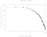
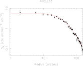
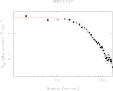
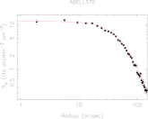
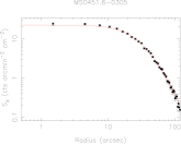
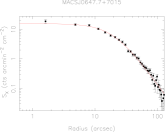
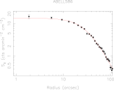
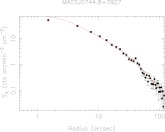
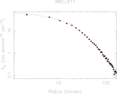
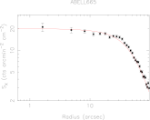
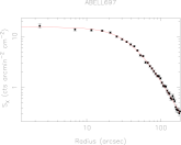
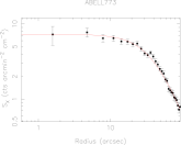
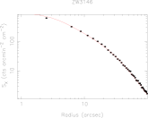
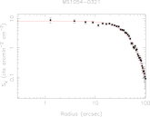
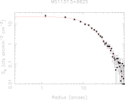
In Figure 6 we show the radial profiles of the X-ray surface brightness for the 38 clusters in our sample. The of the hydrostatic equilibrium model fits to the surface brightness profiles are shown in Table 2.
![[Uncaptioned image]](/html/astro-ph/0512349/assets/x35.png)
![[Uncaptioned image]](/html/astro-ph/0512349/assets/x36.png)
![[Uncaptioned image]](/html/astro-ph/0512349/assets/x37.png)
![[Uncaptioned image]](/html/astro-ph/0512349/assets/x38.png)
![[Uncaptioned image]](/html/astro-ph/0512349/assets/x39.png)
![[Uncaptioned image]](/html/astro-ph/0512349/assets/x40.png)
![[Uncaptioned image]](/html/astro-ph/0512349/assets/x41.png)
![[Uncaptioned image]](/html/astro-ph/0512349/assets/x42.png)
![[Uncaptioned image]](/html/astro-ph/0512349/assets/x43.png)
![[Uncaptioned image]](/html/astro-ph/0512349/assets/x44.png)
![[Uncaptioned image]](/html/astro-ph/0512349/assets/x45.png)
![[Uncaptioned image]](/html/astro-ph/0512349/assets/x46.png)
![[Uncaptioned image]](/html/astro-ph/0512349/assets/x47.png)
![[Uncaptioned image]](/html/astro-ph/0512349/assets/x48.png)
![[Uncaptioned image]](/html/astro-ph/0512349/assets/x49.png)
![[Uncaptioned image]](/html/astro-ph/0512349/assets/x50.png)
![[Uncaptioned image]](/html/astro-ph/0512349/assets/x51.png)
![[Uncaptioned image]](/html/astro-ph/0512349/assets/x52.png)
![[Uncaptioned image]](/html/astro-ph/0512349/assets/x53.png)
![[Uncaptioned image]](/html/astro-ph/0512349/assets/x54.png)
![[Uncaptioned image]](/html/astro-ph/0512349/assets/x55.png)
![[Uncaptioned image]](/html/astro-ph/0512349/assets/x56.png)
![[Uncaptioned image]](/html/astro-ph/0512349/assets/x57.png)
| Cluster | Cluster | Cluster | Cluster | ||||
|---|---|---|---|---|---|---|---|
| CL0016+1609 | 1.38 | Abell 697 | 1.12 | RX J1347.5-1145 | 18.24 | RX J1716.4+6708 | 0.97 |
| Abell 68 | 0.90 | Abell 773 | 0.98 | MS 1358.4+6245 | 2.52 | Abell 2259 | 1.47 |
| Abell 267 | 0.74 | ZW 3146 | 2.43 | Abell 1835 | 3.31 | Abell 2261 | 1.06 |
| Abell 370 | 1.44 | MS 1054-0321 | 1.40 | MACS J1423+2404 | 17.60 | MS 2053.7-0449 | 0.80 |
| MS 0451.6-0305 | 1.28 | MS 1137.5+6625 | 0.71 | Abell 1914 | 15.29 | MACS J2129.4-0741 | 1.24 |
| MACS J0647.7+7015 | 1.07 | MACS J1149.5+2223 | 1.14 | Abell 1995 | 1.23 | RX J2129.7+0005 | 1.15 |
| Abell 586 | 1.30 | Abell 1413 | 1.47 | Abell 2111 | 1.39 | MACS J2214.9-1359 | 1.38 |
| MACS J0744.8+3927 | 1.18 | CL J1226.9+3332 | 1.34 | Abell 2163 | 41.62 | MACS J2228.5+2036 | 1.11 |
| Abell 611 | 1.40 | MACS J1311.0-0310 | 1.47 | Abell 2204 | 3.04 | ||
| Abell 665 | 11.84 | Abell 1689 | 1.25 | Abell 2218 | 1.22 |
Appendix 3: Temperature profiles
| r (arcsec) | Counts | kT (keV) | (dof) |
|---|---|---|---|
| CL 0016+1609 – Obs. 520 | |||
| 0-17 | 2198.3 | 10.2 2.2 | 73.5 (68) |
| 17-24 | 1773.6 | 9.3 2.2 | 64.1 (58) |
| 24-32 | 1671.8 | 9.8 2.3 | 68.7 (54) |
| 32-42 | 2224.6 | 10.1 2.7 | 86.4 (71) |
| 42-52 | 2070.9 | 8.8 1.7 | 84.9 (66) |
| 52-65 | 1946.2 | 9.1 2.0 | 64.6 (67) |
| 65-83 | 1934.0 | 11.1 3.0 | 64.6 (70) |
| 83-101 | 1355.0 | 10.1 3.1 | 39.6 (58) |
| Abell 0068 – Obs. 3250 | |||
| 0-49 | 2036.9 | 10.8 2.8 | 70.5 (67) |
| 49-111 | 1910.0 | 7.5 1.8 | 67.0 (65) |
| Abell 0267 – Obs. 1448 | |||
| 0-53 | 1998.4 | 6.0 0.9 | 71.1 (60) |
| 53-166 | 1658.0 | 5.5 1.2 | 50.6 (65) |
| Abell 0370 – Obs. 515 | |||
| 0-13 | 1071.9 | 9.1 3.1 | 23.4 (37) |
| 13-21 | 1434.9 | 13.3 5.2 | 38.6 (47) |
| 21-28 | 1654.3 | 8.5 2.0 | 67.8 (55) |
| 28-36 | 1842.9 | 9.1 2.3 | 59.4 (59) |
| 36-40 | 965.5 | 8.6 2.6 | 33.6 (34) |
| 40-47 | 1876.2 | 13.1 4.5 | 75.3 (63) |
| 47-55 | 1718.9 | 10.1 3.2 | 72.1 (60) |
| 55-62 | 1591.6 | 7.1 1.7 | 41.3 (57) |
| 62-70 | 1381.4 | 8.5 2.7 | 58.0 (53) |
| 70-81 | 1856.6 | 7.3 1.9 | 63.2 (76) |
| 81-89 | 1004.7 | 6.1 2.3 | 62.3 (46) |
| 89-107 | 1942.2 | 6.8 1.7 | 76.0 (93) |
| 107-134 | 1880.2 | 5.4 1.5 | 129.8 (116) |
| MS 0451.6-0305 – Obs. 529 | |||
| 0-44 | 2002.3 | 7.9 1.5 | 63.3 (62) |
| 44-119 | 1317.6 | 6.8 2.0 | 51.2 (57) |
| MS 0451.6-0305 – Obs. 902 | |||
| 0-14 | 1922.4 | 14.3 4.6 | 41.2 (59) |
| 14-23 | 2226.5 | 9.3 1.9 | 77.5 (67) |
| 23-29 | 1476.1 | 8.3 1.8 | 34.1 (49) |
| 29-38 | 1985.2 | 9.6 2.0 | 73.7 (64) |
| 38-50 | 2171.4 | 10.3 2.4 | 72.8 (71) |
| 50-68 | 2123.6 | 9.1 2.2 | 60.7 (73) |
| 68-101 | 2008.7 | 10.8 4.7 | 116.3 (87) |
| MACS J0647.7+7015 – Obs. 3196 | |||
| 0-37 | 1973.8 | 12.4 3.1 | 56.6 (65) |
| 37-128 | 1323.0 | 10.5 4.5 | 66.3 (65) |
| MACS J0647.7+7015 – Obs. 3584 | |||
| 0-34 | 1885.6 | 10.7 2.4 | 57.3 (60) |
| 34-160 | 1790.8 | 19.1 10.8 | 64.2 (83) |
| Abell 0586 – Obs. 530 | |||
| 0-24 | 1909.4 | 7.8 1.5 | 47.2 (60) |
| 24-43 | 1925.4 | 7.7 1.6 | 75.2 (62) |
| 43-70 | 1939.5 | 6.9 1.2 | 58.8 (63) |
| 70-130 | 2062.0 | 6.4 1.2 | 74.3 (73) |
| MACS J0744.8+3927 – Obs. 3197 | |||
| 0-36 | 1948.1 | 8.47 1.42 | 64.6 (62) |
| 36-125 | 1108.9 | 9.15 4.76 | 59.8 (57) |
| MACS J0744.8+3927 – Obs. 3585 | |||
| 0-41 | 2019.9 | 8.1 1.3 | 96.2 (65) |
| 41-60 | 359.2 | 6.0 2.3 | 18.2 (13) |
| Abell 0611 – Obs. 3194 | |||
| 0-11 | 1916.2 | 6.0 0.8 | 73.9 (60) |
| 11-19 | 1268.4 | 7.3 1.3 | 87.1 (79) |
| 19-24 | 1351.4 | 6.0 1.2 | 44.3 (44) |
| 24-32 | 2341.6 | 6.7 1.3 | 96.8 (74) |
| 32-41 | 1850.1 | 6.0 1.1 | 67.8 (57) |
| 41-49 | 1487.9 | 7.1 1.4 | 52.6 (51) |
| 49-66 | 2279.9 | 5.9 1.0 | 91.4 (78) |
| 66-88 | 1857.0 | 6.0 1.1 | 49.1 (71) |
| 88-126 | 1982.7 | 6.8 2.1 | 121.5 (102) |
| Abell 0665 – Obs. 3586 | |||
| 0-19 | 2240.2 | 7.8 1.4 | 72.3 (69) |
| 19-26 | 1442.0 | 9.2 2.7 | 42.1 (49) |
| 26-37 | 2277.0 | 8.5 1.7 | 94.1 (70) |
| 37-47 | 2140.0 | 7.8 1.4 | 68.2 (67) |
| 47-58 | 2085.3 | 7.7 1.5 | 53.3 (66) |
| 58-69 | 1958.1 | 9.0 2.3 | 80.0 (64) |
| 69-79 | 1950.6 | 9.2 2.3 | 66.5 (66) |
| 79-90 | 1838.9 | 7.4 1.7 | 44.5 (61) |
| 90-100 | 1825.5 | 7.3 1.6 | 48.7 (61) |
| 100-111 | 1727.1 | 9.7 2.9 | 63.4 (59) |
| 111-125 | 2149.2 | 8.3 1.8 | 88.8 (74) |
| 125-139 | 1989.6 | 8.7 2.2 | 78.0 (68) |
| Abell 0665 – Obs. 531 | |||
| 0-37 | 2029.8 | 6.7 1.1 | 58.7 (62) |
| 37-67 | 1904.4 | 8.8 2.2 | 60.3 (60) |
| 67-103 | 2006.3 | 11.9 3.6 | 65.8 (66) |
| Abell 0697 – Obs. 4217 | |||
| 0-25 | 2176.0 | 10.1 2.3 | 67.7 (67) |
| 25-39 | 2031.6 | 10.2 2.6 | 76.6 (63) |
| 39-48 | 1397.5 | 9.1 2.6 | 44.3 (46) |
| 48-67 | 2213.1 | 11.2 2.9 | 74.1 (70) |
| 67-90 | 2117.5 | 10.8 2.8 | 61.4 (70) |
| 90-117 | 2029.7 | 12.6 4.0 | 66.6 (73) |
| 117-154 | 1914.1 | 9.9 2.8 | 81.8 (72) |
| Abell 0773 – Obs. 3588 | |||
| 0-41 | 1930.5 | 6.0 1.0 | 75.2 (61) |
| 41-80 | 1934.3 | 6.2 1.2 | 89.4 (63) |
| 80-157 | 2066.8 | 6.4 1.3 | 72.3 (73) |
| Abell 0773 – Obs. 533 | |||
| 0-36 | 1990.2 | 7.2 1.4 | 66.9 (61) |
| 36-62 | 1900.2 | 8.6 2.1 | 61.3 (61) |
| 62-106 | 2019.5 | 7.1 1.3 | 67.0 (67) |
| ZW 3146 – Obs. 909 | |||
| 0-5 | 3491.4 | 3.9 0.2 | 133 .6 (130) |
| 5-11 | 7557.8 | 4.9 0.2 | 213.8 (154) |
| 11-18 | 8887.2 | 6.5 0.3 | 218.0 (176) |
| 18-25 | 6361.8 | 7.0 0.3 | 180.7 (150) |
| 25-35 | 6237.6 | 8.4 0.6 | 158.3 (150) |
| 35-46 | 5598.2 | 8.2 0.6 | 109.3 (140) |
| 46-60 | 4756.4 | 9.1 0.6 | 153.1 (134) |
| 60-76 | 3401.7 | 9.7 1.2 | 83.5 (109) |
| 76-101 | 3252.7 | 8.7 0.9 | 91.8 (115) |
| 101-140 | 2238.8 | 7.7 1.2 | 101.7 (89) |
| MS 1054-0321 – Obs. 512 | |||
| 0-14 | 740.3 | 13.8 6.3 | 27.7 (26) |
| 14-22 | 937.0 | 7.7 2.6 | 26.1 (33) |
| 22-35 | 1755.5 | 9.6 2.1 | 66.7 (62) |
| 35-50 | 1718.1 | 13.2 4.7 | 65.1 (68) |
| 50-83 | 1751.9 | 8.7 3.5 | 131.7 (109) |
| MS 1137.5+6625 – Obs. 536 | |||
| 0-25 | 1585.5 | 6.4 1.2 | 56.1 (52) |
| 25-75 | 897.7 | 4.6 1.4 | 43.5 (55) |
| MACS J1149.5+2223 – Obs. 1656 | |||
| 0-48 | 1924.1 | 9.30 1.97 | 68.3 (63) |
| 48-108 | 1702.6 | 7.71 1.90 | 50.4 (65) |
| MACS J1149.5+2223 – Obs. 3589 | |||
| 0-46 | 1985.5 | 10.8 2.5 | 64.67 (66) |
| 46-112 | 1911.5 | 7.0 1.6 | 57.6 (71) |
| Abell 1413 – Obs. 1661 | |||
| 0-20 | 2190.8 | 6.0 0.9 | 68.1 (67) |
| 20-34 | 2040.8 | 9.0 2.0 | 63.6 (64) |
| 34-47 | 2005.8 | 8.3 1.5 | 57.0 (64) |
| 47-61 | 1640.5 | 9.2 2.4 | 55.7 (54) |
| 61-79 | 1841.1 | 7.4 1.6 | 57.5 (60) |
| 79-106 | 2156.7 | 6.0 1.0 | 78.4 (68) |
| 106-133 | 1789.5 | 6.2 1.0 | 61.7 (59) |
| 133-178 | 1982.4 | 7.4 1.7 | 76.6 (74) |
| Abell 1413 – Obs. 537 | |||
| 0-18 | 1908.9 | 7.1 1.5 | 55.5 (59) |
| 18-31 | 1973.0 | 8.2 1.8 | 62.3 (62) |
| 31-46 | 2129.7 | 6.2 1.0 | 79.1 (63) |
| 46-62 | 1823.0 | 7.0 1.3 | 49.6 (58) |
| 62-81 | 2045.6 | 9.2 2.3 | 85.3 (65) |
| CL J1226.9+3332 – Obs. 3180 | |||
| 0-82 | 1962.2 | 12.1 2.6 | 58.8 (63) |
| CL J1226.9+3332 – Obs. 932 | |||
| 0-58 | 1003.9 | 15.4 7.5 | 26.9 (35) |
| MACS J1311.0-0310 – Obs. 3258 | |||
| 0-73 | 1963.2 | 6.7 1.1 | 76.3 (65) |
| Abell 1689 – Obs. 1663 | |||
| 0-12 | 2136.8 | 9.4 2.1 | 76.3 (67) |
| 12-17 | 1409.5 | 9.5 2.9 | 47.0 (45) |
| 17-26 | 2928.5 | 9.47 1.81 | 94.7 (87) |
| 26-31 | 1271.1 | 16.57 9.01 | 41.0 (42) |
| 31-41 | 2159.3 | 9.41 2.09 | 65.9 (67) |
| 41-50 | 1922.3 | 9.77 2.69 | 72.0 (63) |
| 50-60 | 1687.4 | 8.72 2.18 | 59.7 (54) |
| 60-74 | 2150.8 | 9.78 2.28 | 75.1 (68) |
| 74-93 | 2244.1 | 14.10 4.95 | 81.6 (72) |
| 93-117 | 2012.4 | 9.22 2.14 | 59.6 (68) |
| 117-146 | 1759.2 | 10.55 3.27 | 56.7 (61) |
| 146-189 | 1532.9 | 6.53 1.57 | 51.2 (59) |
| Abell 1689 – Obs. 540 | |||
| 0-10 | 1601.5 | 11.9 3.8 | 64.8 (51) |
| 10-18 | 2431.2 | 7.8 1.3 | 97.7 (71) |
| 18-24 | 1706.8 | 8.0 1.6 | 47.5 (53) |
| 24-32 | 2236.1 | 13.1 3.8 | 59.1 (68) |
| 32-41 | 1798.6 | 13.4 5.0 | 57.5 (59) |
| 41-52 | 2178.3 | 9.7 2.1 | 82.2 (68) |
| 52-63 | 1890.4 | 11.0 3.0 | 66.6 (60) |
| 63-78 | 2035.9 | 14.7 5.2 | 59.5 (67) |
| 78-94 | 1898.7 | 11.7 4.9 | 61.4 (60) |
| 94-111 | 1371.4 | 12.7 4.7 | 53.0 (46) |
| RX J1347.5-1145 – Obs. 3592 | |||
| 0-2 | 2062.7 | 6.3 0.9 | 95.9 (103) |
| 2-5 | 7479.7 | 8.5 0.7 | 208.3 (166) |
| 5-9 | 6539.0 | 11.2 1.3 | 192.2 (159) |
| 9-12 | 5672.1 | 16.3 3.1 | 199.6 (151) |
| 12-16 | 4939.2 | 14.8 2.9 | 166.5 (137) |
| 16-19 | 4392.6 | 16.8 3.4 | 159.7 (126) |
| 19-23 | 4010.0 | 14.6 3.0 | 106.2 (122) |
| 23-29 | 5869.5 | 13.5 2.0 | 182.8 (154) |
| 29-36 | 4081.0 | 18.4 4.2 | 115.7 (124) |
| 36-47 | 4143.3 | 19.1 4.3 | 158.9 (128) |
| 47-68 | 5440.7 | 14.1 2.5 | 171.7 (154) |
| 68-102 | 4970.9 | 12.8 2.5 | 161.3 (154) |
| MS 1358.4+6245 – Obs. 516 | |||
| 0-7 | 2112.3 | 4.02 0.38 | 61.4 (63) |
| 7-13 | 1629.5 | 5.92 1.18 | 39.3 (50) |
| 13-21 | 2237.5 | 8.36 1.71 | 65.9 (71) |
| 21-29 | 2038.2 | 8.8 1.8 | 63.4 (66) |
| 29-41 | 2143.1 | 9.2 2.2 | 96.1 (68) |
| 41-52 | 1928.4 | 8.6 2.1 | 66.2 (66) |
| 52-66 | 1726.7 | 7.5 2.0 | 50.0 (62) |
| 66-88 | 1959.2 | 8.1 2.3 | 94.3 (82) |
| 88-111 | 1203.9 | 12.6 9.9 | 46.7 (67) |
| Abell 1835 – Obs. 495 | |||
| 0-5 | 4283.1 | 4.3 0.4 | 121.3 (101) |
| 5-9 | 4989.8 | 5.0 0.4 | 117.7 (114) |
| 9-12 | 4033.2 | 6.3 0.7 | 117.6 (104) |
| 12-19 | 6163.1 | 9.1 1.1 | 142.9 (140) |
| 19-26 | 4943.0 | 8.3 1.1 | 143.5 (121) |
| 26-36 | 5573.5 | 9.1 1.2 | 150.2 (133) |
| 36-46 | 4466.6 | 12.6 2.4 | 146.1 (125) |
| 46-64 | 5255.3 | 9.2 1.3 | 116.4 (129) |
| 64-91 | 5233.8 | 11.6 2.2 | 162.7 (142) |
| 901-136 | 4718.5 | 18.4 7.2 | 135.3 (151) |
| Abell 1835 – Obs. 496 | |||
| 0-11 | 5201.4 | 5.0 0.4 | 95.6 (117) |
| 11-20 | 3868.4 | 7.0 0.9 | 111.6 (103) |
| 20-42 | 6416.7 | 8.2 0.9 | 173.9 (142) |
| 42-68 | 4488.9 | 11.2 2.5 | 110.7 (120) |
| 68-138 | 4982.1 | 13.4 4.0 | 139.0 (143) |
| MACS J1423.8+2404 – Obs. 4195 | |||
| 0-3 | 2988.9 | 4.2 0.4 | 97.4 (87) |
| 3-8 | 7992.4 | 4.8 0.3 | 199.7 (146) |
| 8-13 | 4588.5 | 6.6 0.6 | 106.6 (118) |
| 13-18 | 2869.9 | 7.4 1.0 | 66.1 (87) |
| 18-23 | 2169.4 | 7.4 1.2 | 72.9 (66) |
| 23-28 | 1731.4 | 7.2 1.5 | 47.6 (54) |
| 28-32 | 1459.8 | 8.7 2.2 | 52.8 (49) |
| 32-38 | 1140.1 | 6.1 1.4 | 44.2 (41) |
| 38-42 | 943.7 | 7.0 2.2 | 28.9 (37) |
| 42-47 | 739.6 | 6.9 3.3 | 34.1 (29) |
| 47-52 | 657.5 | 5.9 2.1 | 19.5 (28) |
| 52-57 | 553.7 | 7.4 3.9 | 15.9 (25) |
| 57-62 | 484.9 | 6.8 4.2 | 14.5 (24) |
| 62-67 | 477.5 | 7.0 6.5 | 34.0 (24) |
| 67-77 | 806.5 | 5.4 2.0 | 38.3 (47) |
| 77-97 | 1075.9 | 4.6 1.4 | 73.0 (77) |
| Abell 1914 – Obs. 3593 | |||
| 0-24 | 4677.0 | 13.1 2.5 | 125.6 (138) |
| 24-37 | 5716.9 | 11.3 1.7 | 184.5 (154) |
| 37-46 | 4416.5 | 11.0 1.9 | 117.5 (130) |
| 46-55 | 4180.6 | 11.4 2.3 | 117.6 (126) |
| 55-72 | 6022.7 | 8.5 1.1 | 150.1 (152) |
| 72-94 | 4535.4 | 11.5 2.3 | 167.2 (132) |
| 94-138 | 5294.2 | 8.9 1.3 | 144.8 (154) |
| 138-173 | 2636.7 | 8.2 1.8 | 100.7 (93) |
| Abell 1914 – Obs. 542 | |||
| 0-25 | 2276.3 | 10.8 2.7 | 62.5 (69) |
| 25-32 | 1345.1 | 13.4 6.7 | 43.2 (44) |
| 32-44 | 2278.0 | 10.8 2.8 | 55.7 (69) |
| 44-51 | 1613.1 | 16.7 6.8 | 47.9 (53) |
| 51-63 | 2160.2 | 13.6 4.1 | 71.4 (66) |
| 63-78 | 2050.4 | 10.9 3.2 | 65.2 (64) |
| 78-104 | 2186.0 | 8.8 2.2 | 71.7 (69) |
| 104-142 | 1849.5 | 8.4 2.4 | 61.2 (66) |
| Abell 1995 – Obs. 906 | |||
| 0-13 | 2060.1 | 7.8 1.4 | 51.9 (64) |
| 13-17 | 1120.6 | 10.2 4.0 | 38.3 (37) |
| 17-24 | 2658.1 | 7.4 1.3 | 72.9 (78) |
| 24-28 | 1461.6 | 9.3 2.8 | 45.5 (47) |
| 28-36 | 2715.0 | 9.9 2.0 | 60.4 (84) |
| 36-39 | 1293.1 | 13.0 4.9 | 34.5 (43) |
| 39-47 | 2449.4 | 9.1 2.2 | 98.2 (75) |
| 47-54 | 2228.6 | 10.0 2.7 | 86.8 (73) |
| 54-62 | 1814.6 | 7.1 1.3 | 68.4 (61) |
| 62-69 | 1557.0 | 7.2 1.6 | 55.2 (55) |
| 69-84 | 2209.6 | 8.2 2.0 | 83.9 (85) |
| 84-107 | 1992.8 | 11.1 4.6 | 92.1 (92) |
| 107-148 | 1805.4 | 8.4 4.7 | 149.8 (131) |
| Abell 2111 – Obs. 544 | |||
| 0-70 | 2114.6 | 7.5 1.50 | 75.2 (66) |
| 70-163 | 1932.3 | 9.3 3.0 | 87.6 (70) |
| Abell 2163 – Obs. 1653 | |||
| 0-23 | 8821.2 | 18.07 4.57 | 210.6 (201) |
| 23-33 | 9098.7 | 11.62 2.20 | 243.6 (199) |
| 33-43 | 11446.3 | 19.36 4.33 | 256.4 (228) |
| 43-53 | 12904.6 | 12.71 1.89 | 260.6 (243) |
| 53-58 | 6900.5 | 11.4 2.3 | 173.0 (174) |
| 58-68 | 13317.5 | 13.6 1.9 | 231.4 (246) |
| 68-73 | 6111.6 | 11.7 2.1 | 177.8 (164) |
| 73-83 | 11752.2 | 15.0 2.8 | 249.0 (235) |
| 83-93 | 10457.4 | 13.1 2.2 | 231.6 (221) |
| 93-103 | 9532.6 | 16.3 3.7 | 213.3 (212) |
| 103-113 | 8423.0 | 16.5 4.0 | 205.4 (202) |
| 113-129 | 10962.5 | 18.5 4.5 | 257.2 (233) |
| 129-144 | 8863.9 | 14.6 3.1 | 191.3 (207) |
| 144-164 | 10300.9 | 17.1 4.7 | 231.2 (231) |
| 164-184 | 9774.5 | 14.5 3.0 | 275.3 (232) |
| 184-199 | 6843.6 | 18.1 6.1 | 173.2 (195) |
| Abell 2204 – Obs. 499 | |||
| 0-7 | 4961.3 | 3.6 0.2 | 105.5 (114) |
| 7-11 | 4238.5 | 4.3 0.3 | 115.8 (108) |
| 11-19 | 5979.5 | 5.7 0.5 | 166.5 (136) |
| 19-28 | 3962.0 | 8.1 1.2 | 110.2 (111) |
| 28-45 | 6013.9 | 9.4 1.3 | 145.1 (144) |
| 45-62 | 4447.9 | 9.4 1.6 | 118.5 (122) |
| 62-93 | 5059.2 | 10.8 2.0 | 104.3 (137) |
| 93-153 | 5317.6 | 13.4 4.0 | 148.0 (151) |
| Abell 2204 – Obs. 6104 | |||
| 0-6 | 3805.5 | 3.3 0.2 | 125.1 (105) |
| 6-15 | 5643.9 | 5.4 0.4 | 196.7 (142) |
| 15-28 | 5274.9 | 7.3 0.8 | 192.0 (138) |
| 28-45 | 4774.2 | 11.1 1.9 | 130.7 (136) |
| 45-75 | 5517.0 | 9.3 1.2 | 142.9 (151) |
| Abell 2218 – Obs. 1666 | |||
| 0-30 | 5103.0 | 9.2 1.2 | 135.4 (142) |
| 30-46 | 4969.6 | 8.9 1.3 | 128.5 (141) |
| 46-63 | 4936.2 | 8.0 1.1 | 145.5 (140) |
| 63-79 | 4515.1 | 8.3 1.2 | 144.7 (136) |
| 79-107 | 5582.4 | 6.5 0.7 | 151.1 (153) |
| RX J1716.4+6708 – Obs. 584 | |||
| 0-62 | 1428.3 | 7.1 1.6 | 54.2 (57) |
| Abell 2259 – Obs. 3245 | |||
| 0-41 | 1933.3 | 5.3 0.7 | 82.4 (62) |
| 41-79 | 2113.1 | 5.0 0.7 | 67.0 (65) |
| 79-135 | 1830.5 | 5.4 0.9 | 83.3 (63) |
| Abell 2261 – Obs. 550 | |||
| 0-17 | 1801.4 | 6.8 1.4 | 73.1 (57) |
| 17-36 | 2244.5 | 7.4 1.4 | 94.4 (67) |
| 36-59 | 1874.8 | 7.0 1.5 | 50.0 (59) |
| 59-100 | 1957.3 | 9.3 2.2 | 66.9 (67) |
| 100-150 | 1140.8 | 5.8 1.6 | 38.2 (47) |
| MS 2053.7-0449 – Obs. 1667 | |||
| 0-86 | 1095.1 | 3.8 0.9 | 36.0 (57) |
| MS 2053.7-0449 – Obs. 551 | |||
| 0-117 | 1188.4 | 6.7 2.8 | 87.4 (79) |
| MACS J2129.4-0741 – Obs. 3199 | |||
| 0-46 | 2012.3 | 7.1 1.1 | 63.4 (66) |
| 46-90 | 651.2 | 5.5 1.7 | 38.7 (30) |
| MACS J2129.4-0741 – Obs. 3595 | |||
| 0-42 | 1974.1 | 12.3 2.9 | 55.6 (65) |
| 42-90 | 875.8 | 8.7 3.7 | 41.2 (37) |
| RX J2129.7+0005 – Obs. 552 | |||
| 0-14 | 1852.5 | 4.4 0.5 | 57.2 (57) |
| 14-34 | 2160.4 | 6.1 0.9 | 65.9 (65) |
| 34-67 | 1931.2 | 6.4 1.0 | 75.4 (64) |
| 67-159 | 1970.1 | 7.4 1.6 | 85.2 (73) |
| MACS J2214.9-1359 – Obs. 3259 | |||
| 0-32 | 1882.6 | 9.5 2.4 | 64.2 (60) |
| 32-95 | 2099.3 | 15.1 5.0 | 82.1 (76) |
| MACS J2214.9-1359 – Obs. 5011 | |||
| 0-40 | 2030.9 | 10.6 2.8 | 75.4 (64) |
| 40-119 | 1691.7 | 8.6 2.6 | 50.0 (67) |
| MACS J2228.5+2036 – Obs. 3285 | |||
| 0-29 | 1835.3 | 8.4 1.7 | 58.5 (59) |
| 29-68 | 2140.5 | 8.9 1.9 | 53.3 (68) |
| 68-126 | 1605.8 | 10.5 3.6 | 57.8 (67) |