$L_{\rm X}-T$ RELATION AND RELATED PROPERTIES OF GALAXY CLUSTERS

Abstract

An observational approach is presented to constrain the global structure and evolution of the intracluster medium based on the ROSAT and ASCA distant cluster sample. From statistical analysis of the gas density profile and the connection to the $L_{\rm X}-T$ relation under the $\beta$-model, the scaled gas profile is found to be nearly universal for the outer region and the luminosity evaluated outside $0.2r_{500}$ is tightly related to the temperature through $\propto T^{\sim 3}$ rather than $T^{2}$. On the other hand, a large density scatter exists in the core region and there is clearly a deviation from the self-similar scaling for clusters with a small core size. A direct link between the core size and the radiative cooling timescale, $t_{\rm cool}$ and the analysis of X-ray fundamental plane suggest that $t_{\rm cool}$ is a parameter to control the gas structure and the appearance of small cores in regular clusters may be much connected with the thermal evolution. We derive the luminosity-‘ambient temperature’ relation ($L_{\rm X}-T^{\prime}$), assuming the universal temperature profile for the clusters with short cooling time and adopting a correction $T^{\prime}=1.3T$, and find the dispersion around the relation significantly decreases in comparison to the case of the $L_{\rm X}-T$ and the slope becomes less steep from $3.01^{+0.49}_{-0.44}$ to $2.80^{+0.28}_{-0.24}$. $L_{\rm 1keV}$, which is defined as a normalization factor for each cluster, can be regarded as constant for a wide range of the cooling time. We further examined the $L_{\rm X}-T\beta$ and $L_{\rm X}-T^{\prime}\beta$ relations and showed a trend that merging clusters segregate from the regular clusters on the planes. A good correlation between the cooling time and the X-ray morphology on the $L_{\rm 1keV}-(t_{\rm cool}/t_{\rm age})$ plane leads us to define three phases according to the different level of cooling, and draw a phenomenological picture: after a cluster collapses and $t_{\rm cool}$ falls below the age of the universe, the core cools radiatively with quasi-hydrostatic balancing in the gravitational potential, and the central density gradually becomes higher to evolve from an outer-core-dominant cluster, which marginally follows the self-similarity, to inner-core-dominant cluster.

1 INTRODUCTION

The X-ray luminosity-temperature ($L_{\rm X}-T$) relation of galaxy clusters is one of the most fundamental parameter correlations, established from previous X-ray observations (e.g. Edge et al., 1990). Since the X-ray luminosity reflects temperature and density profiles of hot intracluster medium (ICM), the $L_{\rm X}-T$ relation should contain information on physical status and evolution of the ICM.

Observationally, the correlation is well approximated with a power-law function: $L_{\rm X}\propto T^{\alpha}$, with $\alpha\sim 3$ (e.g. Edge et al., 1990; David et al., 1993; Markevitch, 1998; Arnaud & Evrard, 1999). In addition, it shows a significant scatter around the mean power-law relation and little redshift evolution. On the other hand, the self-similar model (e.g. Kaiser, 1986) predicts $\alpha=2$. Thus the inconsistency between the observations and the simple theoretical model has been debated for many years and various possibilities including non-gravitational heating (e.g. Evrard & Henry, 1991; Cavaliere, Menci, & Tozzi, 1997) and dependence of gas mass or gas-mass fraction on the temperature have been proposed (e.g. David et al., 1993; Neumann & Arnaud, 2001). Recently, hydrodynamical simulations have indicated that the effect of radiative cooling plays an important role to reproduce the observed $L_{\rm X}-T$ relation (e.g. Muanwong et al., 2002). They also suggested a further requirement of significant non-gravitational heating mechanism so as to account for the observed gas-mass fraction, however, the physical origin of the additional heating is yet to be understood.

Under the virial theorem and the isothermal $\beta$-model (Cavaliere & Fusco-Femiano, 1976), an ICM temperature $T_{\rm gas}$ is proportional to a virial temperature, $T_{\rm vir}$, and differs by a factor of $\beta$, $T_{\rm vir}\sim T_{\rm gas}\beta$. However, since $T_{\rm gas}$ is usually an emission-weighted temperature measured from X-ray spectroscopy and strongly reflects the temperature of the cluster core region, a temperature decrease due to radiative cooling may have much influence on the $T_{\rm gas}$ measurement. The ASCA spectroscopy of central region of clusters particularly with cD galaxy provided important results that cool emission from the core is systematically less luminous than that estimated in the past mainly on the basis of imaging observations (e.g. Makishima et al., 2001). After the advent of the XMM-Newton and Chandra X-ray satellites, more detailed temperature profiles have been measured for nearby ‘cooling-flow’ clusters, which typically show central temperature decrement by a factor of $\sim 2$ (e.g. Kaastra et al., 2004). These facts gave a piece of evidence against the standard cooling-flow model (Fabian, 1994), which triggered explorations of a variety of new scenarios for gas heating: heat conduction from outer hot layers (e.g. Narayan & Medvedev, 2001), AGN heating (e.g. Böhringer et al., 2002), magnetic reconnections (Makishima, 1997), Tsunami (Fujita et al., 2004) etc. Recently Masai & Kitayama (2004) proposed a quasi-hydrostatic model for cluster gas under radiative cooling, which predicts a characteristic temperature profile with an asymptotic temperature for the central region being $\sim 1/3$ of the non-cooling outer region. Their calculation agrees well with that observed in the cooling-flow clusters. If the ‘universal’ temperature profile emerges in all or a fraction of clusters with short cooling timescales, the effect of temperature drop should be properly taken into account in the discussion of the $L_{\rm X}-T$ relation.

Another point is due to a connection of the $L_{\rm X}-T$ relation to the cluster core sizes. Ota & Mitsuda (2002) found based on the X-ray data analysis of 79 distant clusters with ROSAT and ASCA that the distribution of the cluster core radius shows two distinct peaks at $\sim 50$ kpc and $\sim 200$ kpc for $H_{0}=70$. When dividing the sample into two subgroups corresponding to the two peaks, they show a significant difference in the normalization factor of the $L_{\rm X}-T$ relation. Some possibilities have been discussed to understand the origin of the double-peaked distribution (Ota & Mitsuda, 2002, 2004), however, it is yet to be clarified. As long as one rely on the hydrostatic equilibrium and the isothermal $\beta$-model, their result may indicate that underlying dark matter distribution is likely to have two preferable scales of 50 kpc and 200 kpc. On the other hand, it is also found that the core radius is tightly related to the radiative cooling timescale (e.g. Ota & Mitsuda, 2004; Akahori & Masai, 2005). Thus the core structure might largely be a result of the thermal evolution of the ICM.

In this paper, using a large number of ROSAT and ASCA clusters compiled by Ota (2001); Ota & Mitsuda (2004), we investigate correlations between the fundamental cluster parameters. Since ASCA has a high sensitivity to measure the X-ray spectrum in the wide energy band while ROSAT is good at imaging in the soft X-ray band, the two observatories are an excellent combination to study properties of the intracluster medium. At present the XMM-Newton and the Chandra satellites are in orbit and generate much cluster data with higher sensitivities. However, the data set used in the present paper will be one of the best existing to construct the largest sample of distant clusters and study global X-ray structures. While Ota & Mitsuda (2002) mainly focused on the discovery of the typical two core sizes based on the analysis of 79 distant clusters with ROSAT and ASCA, Ota & Mitsuda (2004) described the uniform analysis, and showed the X-ray parameters for the individual clusters and the results on scaling relations. The present paper addresses the $L_{\rm X}-T$ relation in more detail, which is organized as below. In § 2, the sample and parameter estimation are described. In § 3, we show gas density profiles of the sample and how they are related to a scatter about the $L_{\rm X}-T$ relation. Since redshift evolution is not clearly seen in the present distant sample and our analysis is based on a conventional $\beta$-model, a study of redshift evolution in the $L_{\rm X}-T$ relation is beyond the scope of the present paper. In § 4 and § 5, we mainly focus on the $L_{\rm X}-T$ relation and show its connection with the cluster core radius and the cooling time. In § 6 we also derive a $L_{\rm X}-T\beta$ relation and show a trend that possible merging clusters segregate from regular clusters on the plane. Finally in § 7, major results are summarized and the evolution of the ICM are discussed particularly in the light of radiative cooling.

We use $\Omega_{\rm M}=0.3$, $\Omega_{\Lambda}=0.7$ and $h_{70}\equiv H_{0}/(70~{}{\rm km\,s^{-1}Mpc^{-1}})=1$. The quoted parameter errors are the 90% confidence range throughout the paper unless otherwise noted. The $1\sigma$ error bars are plotted in all figures.

2 SAMPLE AND PARAMETER ESTIMATIONS

2.1 The Sample

The sample is selected from an X-ray catalogue of the ROSAT and ASCA distant clusters presented in Ota & Mitsuda (2004). Though the original catalogue includes 79 clusters in the redshift range of $0.1<z<0.82$, the final sample used in this work comprises 69 clusters in $0.10\leq z\leq 0.56$ in order to reduce possible selection effect and measurement uncertainties which are more serious at higher redshifts, as detailed below.

Because the sample was collected from the archival data of the pointing observations, in order to reduce the selection effect that is not negligible at higher redshift, we exclude 5 high-redshift clusters with large measurement uncertainties from the Ota & Mitsuda (2004) sample: they are #75 MS2053.7-0049 (catalog ), #76 3C220.1 (catalog ), #77 MS1137.5+6625 (catalog ), #78 RXJ1716.6+6708 (catalog ), #79 MS1054.5-0321 (catalog ) (see Ota & Mitsuda (2004) for details). We exclude #71 3C295 (catalog ) and #76 3C220.1 (catalog ) due to possible contaminations of X-ray emission from the central radio sources as reported by Chandra observations (see Allen et al. (2001a) for 3C295 (catalog ) and Worrall et al. (2001) for 3C220.1 (catalog )), and #56 CL0500-24 (catalog ), #61 CL2244-02 (catalog ), and #66 CL0024+17 (catalog ) due to uncertainties in the spectroscopy caused by contaminations from point sources. We did not use #43 A1758 and #79 MS1054.5-0321 because their $\beta$-model parameters were not well constrained.

2.2 Brief Summary of X-ray Data Analyses

The data analyses consisted of two major steps: 1) the spatial analysis with the ROSAT HRI and 2) the spectral analysis with the ASCA GIS and SIS.

For 1), the radially-averaged X-ray surface brightness distribution was fitted with the isothermal $\beta$-model to determine the slope parameter $\beta$, the core radius $r_{c}$ and the central surface brightness. The model gave an reasonably good fit to the observed surface brightness of many clusters: it resulted in a statistically acceptable fit for about 2/3 of the sample. For some clusters, however, it has left residual emission in the central region and a significant improvement was found when including an additional $\beta$-model component particularly for 9 clusters (termed as “double-$\beta$” clusters). We have further found that adoption of the single $\beta$-model for such double-$\beta$ clusters will return parameters consistent with one of the two $\beta$-model components, as shown in Fig. 9 of Ota & Mitsuda (2004), which means the single $\beta$-model tends to pick up a component that dominates the emission. Thus the present work basically stands on the single $\beta$-model for the reason that we are mainly interested in a systematic study on the global structure in a large number of distant clusters. Note that possible systematic errors of physical parameters estimated under the $\beta$-model will be discussed in the next subsection. Furthermore, the X-ray morphology was measured with using ‘centroid variations’ of the cluster image and the sample was classified into “regular” and “irregular” clusters (see §3.2 of Ota & Mitsuda (2004) for details).

For 2), the emission-weighted temperature and bolometric luminosity were measured from the ASCA spectroscopic data under the Raymond-Smith model (Raymond & Smith, 1977), utilizing the XSPEC software version 9.0. $kT$ is the emission-weighted temperature determined from the simultaneous fitting to the ASCA GIS and SIS spectra extracted from $r<6\arcmin$ and $r<3\arcmin$ circular regions, respectively, and the bolometric luminosity, $L_{\rm X}$ is calculated within a virial radius $r_{500}$. Here $r_{500}$ is defined as the radius within which the average matter density is equal to $\Delta_{c}=500$ times the critical density of the Universe at the cluster redshift.

In what follows, we use the X-ray parameters derived under the single $\beta$-model; the slope parameter $\beta$, the core radius $r_{c}$, the central electron density $n_{e0}$, and the radiative cooling time $t_{\rm cool}$ as well as spectroscopically measured $T$ and $L_{\rm X}$. All quantities are listed in Tables 2, 4, and 5 of Ota & Mitsuda (2004).

2.3 Parameter Estimation under the $\beta$-model and systematic errors

To perform a reliable estimation of the $\beta$-model parameters, we have carefully checked the effect of the ROSAT/HRI PSF on the spatial analysis. As detailed in § 3.4 of Ota & Mitsuda (2004), we confirmed that the effect is negligibly small and the parameters are well reproduced as long as $r_{c}$ is larger than $5\arcsec$. We have also checked the consistency with the previously published values from the Chandra observations in regard to the $\beta$-model parameters ($\beta$ and $r_{c}$) and the temperature, and found a good agreement (see § 3.4 and § 4.2 of Ota & Mitsuda (2004)). Due to the large ASCA PSF, it is not easy to measure the temperature profile accurately for the distant clusters. We then use the spectroscopically determined mean temperature in the parameter estimation. We will further evaluate possible systematic errors in estimating physical parameters under the $\beta$-model, $L_{\rm X}$ and $t_{\rm cool}$, which are important quantities in the present study.

• $L_{\rm X}$
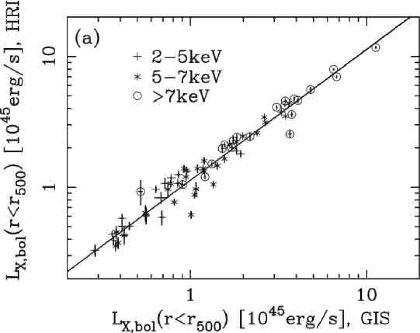
  To estimate a systematic error of $L_{\rm X}$, we first calculate the bolometric luminosity within $r<6\arcmin$ in two different ways: 1) convert the 2–10 keV luminosity measured with the GIS spectrum into the bolometric luminosity using the emissivity of the Raymond-Smith plasma model and the ASCA temperature, and 2) integrate the $\beta$-model surface brightness distribution determined with the ROSAT HRI within the same integration area and multiply it by the band correction factor. We found that two estimations are consistent within about 10–20% in all three different temperature ranges of 2–5, 5–7, $>7$ keV or four different redshift ranges, 0.1–0.2, 0.2–0.3, 0.3–0.4, $>0.4$. This also assures that the current assumption of the isothermal $\beta$-model gives reasonably a good approximation to the real clusters in estimating $L_{\rm X}$. Then we finally determine the bolometric luminosity within $r_{500}$, $L_{\rm X}$ from 1) the bolometric luminosity that was spectroscopically measured within $6\arcmin$ under the Raymond-Smith model and corrected for the emission from outside $6\arcmin$ by assuming the $\beta$-model surface brightness distribution. In Fig. 1a we show a comparison of the bolometric luminosities measured with GIS and HRI.

• $t_{\rm cool}$
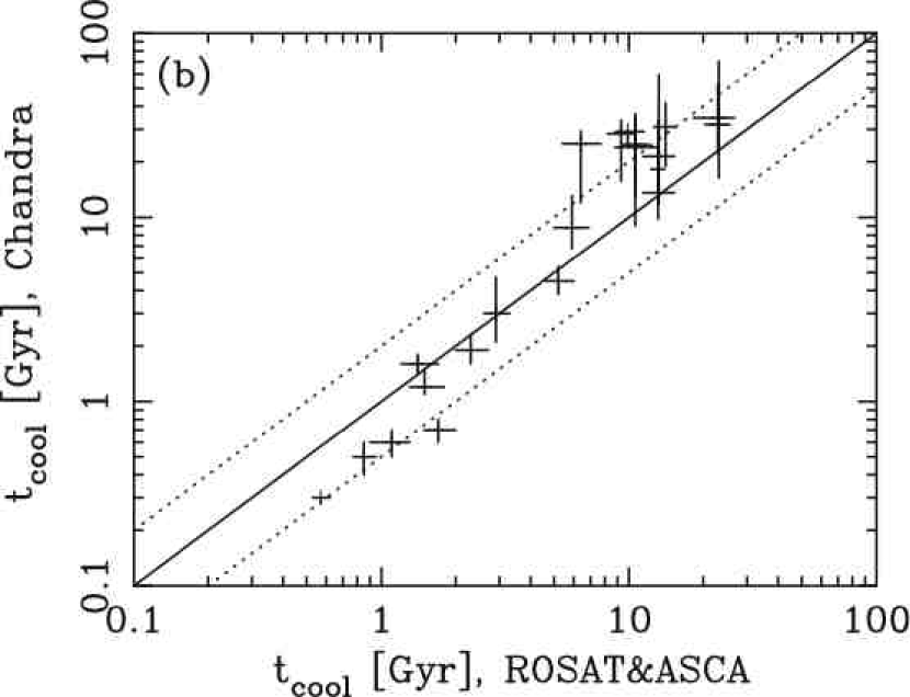
  In the temperature range concerned, the cooling rate of the gas is dominated by free-free emission and then approximately proportional to $\sqrt{T}$. Therefore, with the cooling rate in the form $q_{\rm ff}\sqrt{T}n_{e0}^{2}$, we define the cooling time for a cluster as $t_{\rm cool}=3k\sqrt{T}/q_{\rm ff}n_{e0}$, where $n_{e0}$ is the gas density at the cluster center. On the other hand, recent higher-resolution observations of clusters with a cooling core pointed that the conventional $\beta$-model does not sufficiently fit overall profiles (e.g. Lewis et al., 2003; Hicks et al., 2002). In addition, if the central temperature drop by a factor of $\sim 2$ exists like what observed in many cooling-flow clusters, it might cause an overestimation of $t_{\rm cool}$. We then make a comparison with recent results from Bauer et al. (2005) as they analyzed Chandra data of X-ray luminous clusters at $0.15<z<0.4$ and derived the cooling time profiles using spatially resolved spectral information. From Fig. 1b, we find that there is an agreement between the two analyses: for 11 out of 21 distant clusters $t_{\rm cool}$ is consistent with the Chandra results within the measurement errors. For the rest of them, it is systematically larger (smaller) for $t_{\rm cool}\lesssim 2$ Gyr ($t_{\rm cool}\gtrsim 10$ Gyr). As the clusters with $t_{\rm cool}\gtrsim 10$ Gyr are mostly irregular ones, the underestimation might be due to their complex internal structure and different definitions of the centroid position. From temperature maps derived by Bauer et al. (2005), we found that clusters with systematically smaller $t_{\rm cool}$ tend to have hot spots at the centroids or gas hotter than the surrounding regions. This would then bias the temperature toward lower value (as we use the emission-weighted temperature instead of the spatially-resolved central temperature) and then higher central density (to account for the observed emission measure), resulting in shorter $t_{\rm cool}$. For clusters with $t_{\rm cool}\lesssim 2$ Gyr, the overestimation may be attributed to possible temperature decrease at the center: assuming that the central temperature is 1/2 – 1/3 of ambient temperature, $T^{\prime}$, and the emission-weighted temperature is related through $T\sim T^{\prime}/1.3$ (Eq. 21 in § 5.2), $t_{\rm cool}$ is possibly overestimated by a factor of $\sim 1.3-1.8$. Thus this may reconcile the factor of $\sim 2$ difference seen in Fig. 1b. However, because the above estimation depends on the assumed temperature profile, we use $t_{\rm cool}$ obtained from the $\beta$-model analysis of the ROSAT and ASCA data. Note that the two analyses compared in Fig. 1b are consistent within at most a factor of 2 and our discussion is not so much affected by the absolute value of $t_{\rm cool}$ as this paper aims at a study of a global trend of the ICM evolution, which is suggested to proceed along the “principal axis” (§ 4.4) over two orders of magnitudes of cooling time.

3 $L_{\rm X}-T$ RELATION AND GAS DENSITY PROFILES

3.1 Core Radius Distribution and $r_{500}-r_{c}$ Relation

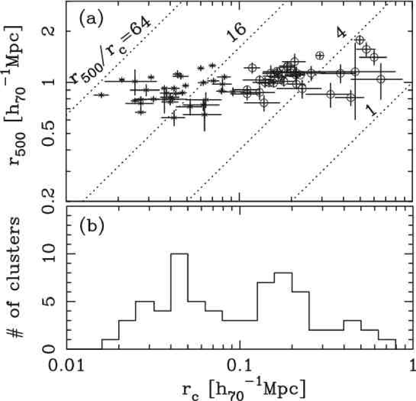
Since the $L_{\rm X}-T$ relation is sensitive to the structure of the cluster core region, we first examine the core radius. As noted in Ota & Mitsuda (2002), together with 45 nearby clusters analyzed in Mohr, Mathiesen & Evrard (1999), the $r_{c}$ distribution of 121 clusters exhibits high concentrations around $50~{}h_{70}^{-1}$kpc and $200~{}h_{70}^{-1}$kpc . We show the core radius distribution of the present sample in Fig. 2b. Though the $r_{c}$ has a large cluster-to-cluster dispersion, we find that about 60% of clusters are included in narrow ranges corresponding to the two peaks. Thus the large dispersion is partly due to the double peak structure of the $r_{c}$ distribution.

Under the self-similar model, the internal structure of the gas should be scaled by the virial radius, and then $r_{500}/r_{c}$ should be constant for all clusters. However, as is seen from Fig. 2a, $r_{c}$ does not simply scaled by $r_{500}$. As mentioned in Ota & Mitsuda (2004), we should be careful about the results of the $r_{500}-r_{c}$ relation because it depends on the choice of the $r_{c}$ range. When we fit all the sample at the same time, we obtain a weak correlation, $r_{500}\propto r_{c}^{0.15\pm 0.04}$ ($\chi^{2}/{\rm d.o.f.}=953.2/67$). Since $r_{500}/r_{c}\gg 1$ in general, $r_{500}$ is mostly determined by the temperature. Actually $r_{c}$ and $T$ do not show a strong correlation. If we divide the sample into two $r_{c}$ groups relative to $r_{c}=100$ kpc, $r_{500}\propto r_{c}^{0.37^{+0.12}_{-0.11}}$ for 34 clusters with $r_{c}>100$ kpc ($\chi^{2}/{\rm d.o.f.}=107.7/32$) while no meaningful correlation was found for 35 clusters with $r_{c}<100$ kpc (the correlation coefficient is 0.21). We further restrict the large core group to a narrow range, for example $100<r_{c}<200$ kpc, $r_{500}\propto r_{c}^{0.71^{+0.52}_{-0.27}}$ ($\chi^{2}/{\rm d.o.f.}=21.0/16$). Thus we consider that the large core clusters may marginally satisfy the self-similar condition (see also Akahori & Masai (2005)). On the other hand, since the small core group clearly shows a deviation from the $r_{500}-r_{c}$ relation, the formation of the small cores is suggested to be determined from some physical process other than the self-similar collapse. Furthermore, for 6 clusters with a very large core radius of $r_{c}>400$ kpc, which forms the third peak around 500 kpc in the $r_{c}$ histogram (Fig. 2b), there is no meaningful $r_{500}-r_{c}$ correlation (the correlation coefficient is 0.21). Thus they do not satisfy the self-similarity. This deviation may be attributed to the past or on-going merging events, which we will discuss in more detail in § 6.1.

3.2 Scaled Gas Density Profiles

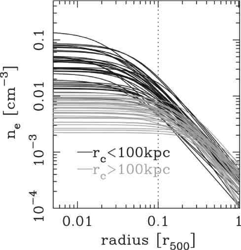
To investigate the global gas density structure, we plot the best-fit $\beta$-model profiles for 69 clusters in Fig. 3, where the radius was normalized by $r_{500}$. A significant scatter of the density exists within $\sim 0.1r_{500}$ region (typically $0.1r_{500}\sim 100$ kpc) and the smaller core clusters show a systematically higher density in comparison to the large core clusters. On the other hand, the profiles are fairly universal outside that radius. We consider that this is consistent with the similarity found in outer regions of scaled profiles for nearby clusters (Neumann & Arnaud, 1999).

In the next two subsections we will treat the core region and the envelope separately in order to directly show how the density profile is related to the scatter around the $L_{\rm X}-T$ relation. We found that the $r_{500}-r_{c}$ relation and the density profile do not show a clear evolution against the observed redshift. However it is important to test whether the $L_{\rm X}-T$ relation would evolve with redshift or it is more closely related with other physical parameters. Then in § 3.5 we will investigate the redshift dependence of the $L_{\rm X}-T$ relation since the present sample covers the redshift range of $0.1<z<0.56$.

3.3 $L_{\rm X}-T$ outside $0.2r_{500}$

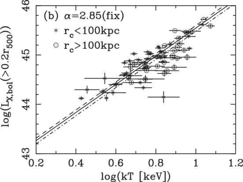
We calculate the luminosities outside a radius of $0.2r_{500}$ and plot them against the temperature in Fig. 4b. The radius was chosen so as to be a typical $r_{c}$ of the large core clusters, $\sim 200$ kpc and thus the emission from the core region can be removed from the overall emission. As a result, we obtained

$$L_{\rm X}(>0.2r_{500})=4.95^{+3.45}_{-2.13}\times 10^{42}(kT)^{2.85^{+0.30}_{-0.27}}.$$ (1)

We found that there is no significant difference in the relation between the two $r_{c}$ groups (see also Table 1) and the data scatter around the mean relation is surprisingly small. Despite the similarity of the outer profiles shown in §3.2, however, the measured power-law index is yet close to 3 rather than the self-similar expectation of 2. This is also true for 20 clusters with $100<r_{c}<200$ kpc, which marginally satisfy the self-similar relation as noted in § 3.1; the power-law index is $3.13^{+0.58}_{-0.51}$.

Note that the $L_{\rm X}-T$ relation is highly sensitive to the way the central emission is treated. Allen & Fabian (1998) pointed out that the slope of the $L_{\rm X}-T$ relation would be flattened from $T^{3}$ to $T^{2}$ once corrected the central emission based on the standard cooling flow model. We find that the slope is still steeper than the prediction of the self-similar model by simply excluding the central component in a model-independent manner.

3.4 $L_{\rm X}-T$ inside $0.2r_{500}$

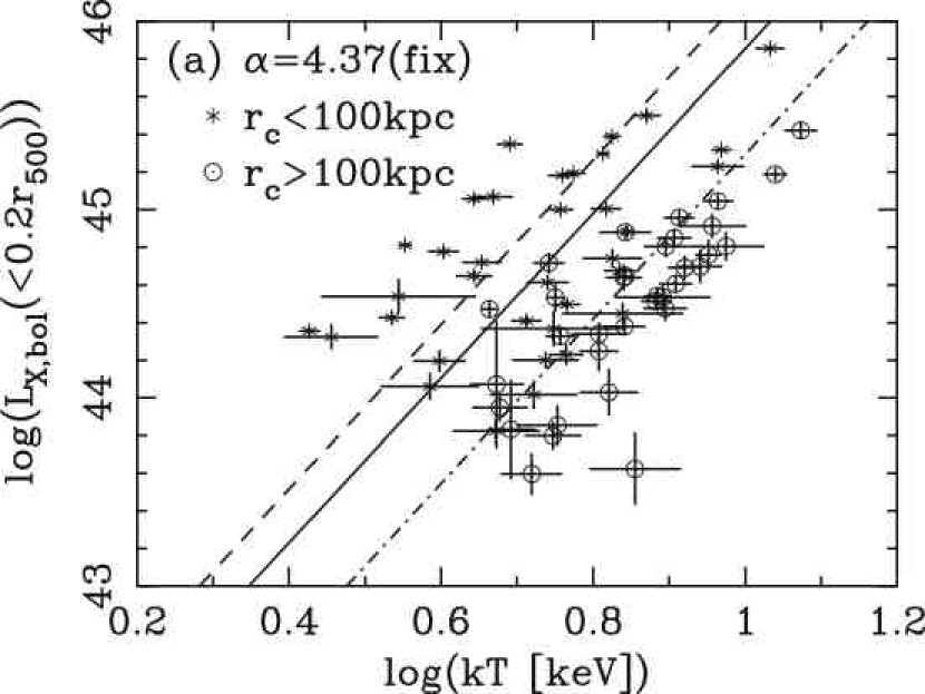
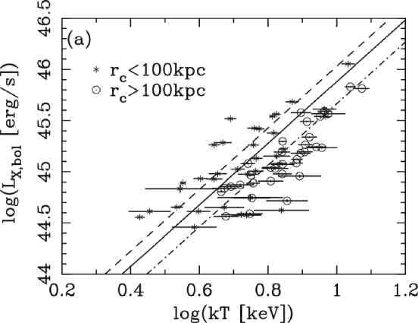
In Fig. 4a, we show the $L_{\rm X}-T$ relation calculated for $r<0.2r_{500}$. The power-law fitting resulted in

$$L_{\rm X}(<0.2r_{500})=3.02^{+45.22}_{-2.83}\times 10^{41}(kT)^{4.37^{+1.54}_{-1.50}}.$$ (2)

There is a significant data scatter in the plot and the luminosity is systematically higher for the small core group for a fixed temperature. If assuming the best-fit slope of 4.37, the relations for the small and large core groups are obtained as:

$$L_{\rm X}(<0.2r_{500}) = 5.82^{+1.91}_{-1.12}\times 10^{41}(kT)^{4.37}~{}{\rm for}~{}r_{c}\leq 0.1~{}{\rm Mpc},$$ (3)

$$L_{\rm X}(<0.2r_{500}) = 8.32^{+1.58}_{-1.57}\times 10^{40}(kT)^{4.37}~{}{\rm for}~{}r_{c}>0.1~{}{\rm Mpc}$$ (4)

(see also Table 1). This significant difference in the normalization factor can be attributed to a negative correlation between the central density and the core radius as mentioned in §3.2.

We then see from Figs. 3 and 4 that the density scatter inside $0.2r_{500}$ is indeed a source of scatter seen in the $L_{\rm X}-T$ relation. In comparison to the result for $r>0.2r_{500}$, the large variety of the luminosity for $r<0.2r_{500}$ and the significant deviation from the self-similarity for the small core clusters may imply that the dispersion around the $L_{\rm X}-T$ is closely related to the evolution of the ICM in the central region after the collapse.

3.5 Redshift Dependence of $L_{\rm X}-T$ and Comparison to Previous Results

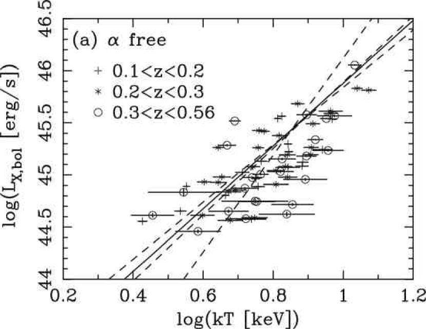
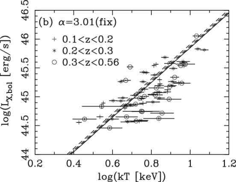
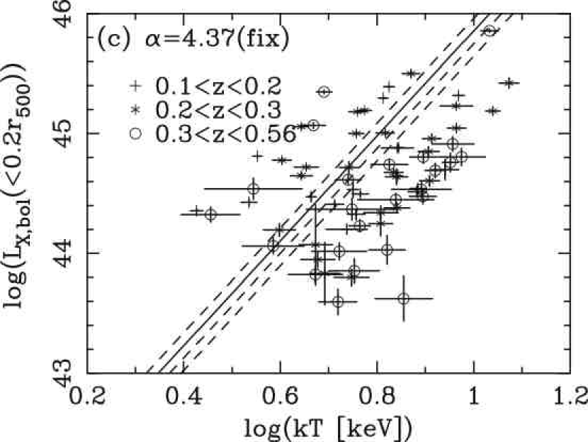
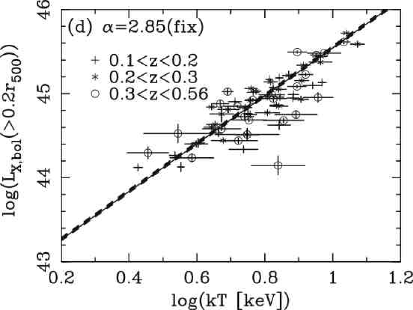
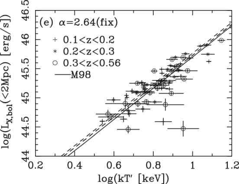
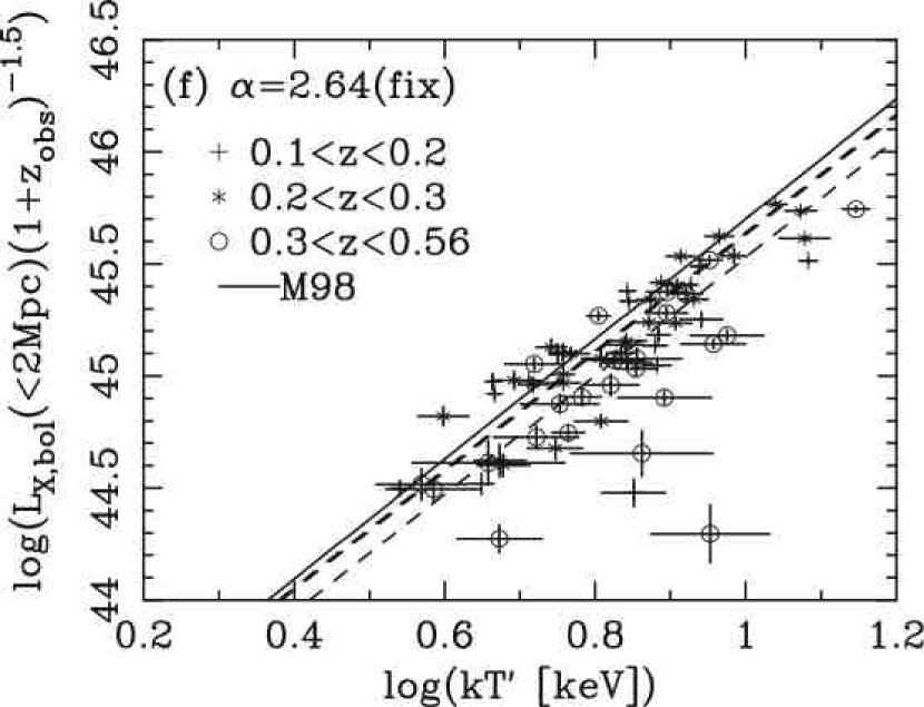
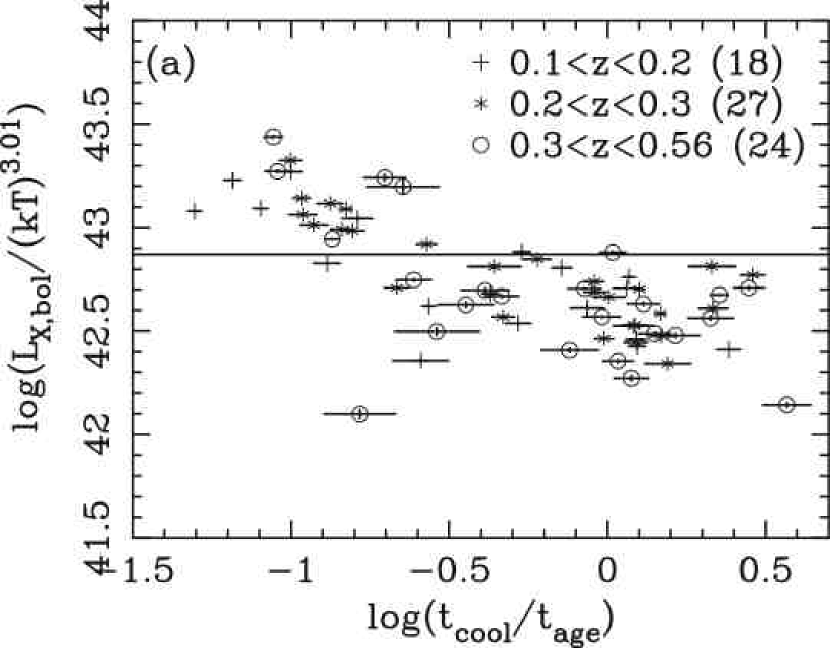
We investigate the redshift dependence of the $L_{\rm X}-T$ relation by evaluating the relations for the following three subsets of data: 18 clusters in $0.1\leq z<0.2$, 27 clusters in $0.2\leq z<0.3$, and 24 clusters in $0.3\leq z<0.56$ (only 7 out of 24 have $z>0.4$) and compare with the previous results on high-redshift ($z>0.4$) and low-redshift ($z<0.1$) clusters. To constrain the redshift dependence in the core and outer region separately, we also derive the $L_{\rm X}-T$ relation for $r<0.2r_{500}$ and $r>0.2r_{500}$. We did not apply the evolution correction to $L_{\rm X}$ (i.e. multiplying $L_{\rm X}$ by $E(z)^{-1}$ since it does not significantly change the relation for $\Delta_{c}=500$ as shown in Table 9 of Ota & Mitsuda (2004).)

• $L_{\rm X}-T$ relation
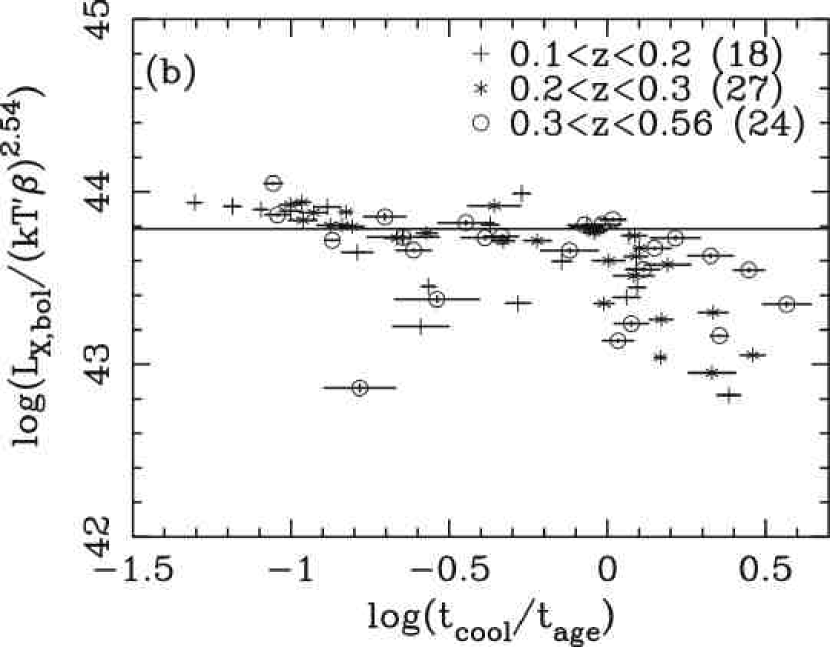
  The power-law fitting of the $L_{\rm X}(<r_{500})-T$ relations for three redshift subgroups resulted in

  $$L_{\rm X} = 1.23^{+2.62}_{-0.95}\times 10^{43}(kT)^{2.75^{+0.85}_{-0.71}}~{}{\rm for}~{}0.1\leq z<0.2,$$ (5)

  $$L_{\rm X} = 5.13^{+19.0}_{-4.23}\times 10^{42}(kT)^{3.18^{+0.92}_{-0.84}}~{}{\rm for}~{}0.2\leq z<0.3,$$ (6)

  $$L_{\rm X} = 2.95^{+108.5}_{-2.92}\times 10^{41}(kT)^{4.65^{+2.33}_{-1.86}}~{}{\rm for}~{}0.3\leq z<0.56$$ (7)

  (Fig. 5a). There is a marginal trend to obtain a steeper slope and a smaller normalization factor for the higher redshfit clusters. However, because of the large uncertainties seen in the slope parameter, if fixed at the best-fit value of the total sample, 3.01, the normalization factors overlap with each other within the errors as shown in Eqs. 8–10 and Fig. 5b, and thus the redshift dependence is not clear in the observed redshift range.

  $$L_{\rm X} = 7.94^{+1.37}_{-1.17}\times 10^{42}(kT)^{3.01}~{}{\rm for}~{}0.1\leq z<0.2,$$ (8)

  $$L_{\rm X} = 7.08^{+0.71}_{-1.23}\times 10^{42}(kT)^{3.01}~{}{\rm for}~{}0.2\leq z<0.3,$$ (9)

  $$L_{\rm X} = 6.92^{+1.32}_{-1.60}\times 10^{42}(kT)^{3.01}~{}{\rm for}~{}0.3\leq z<0.56.$$ (10)

  Ettori et al. (2004) reported a steep slope of $3.72\pm 0.47$ ($1\sigma$ error) for high redshift clusters ($0.4<z<1.3$) based on the Chandra data analysis and suggested a negative evolution. Eqs. 6 and 7 agree with their relation within the errors. Thus there might be a weak redshift evolution in the $L_{\rm X}-T$ relation. However, due to the large uncertainties associated with the relations for the higher redshifts, it is not statistically significant.

• $L_{\rm X}(<0.2r_{500})-T$ and $L_{\rm X}(>0.2r_{500})-T$ relations
  We obtain the $L_{\rm X}(<0.2r_{500})-T$ relation in the three redshift ranges as follows (see also Fig. 5c).

  $$L_{\rm X}(<0.2r_{500}) = 3.89^{+2.53}_{-1.53}\times 10^{41}(kT)^{4.37}~{}{\rm for}~{}0.1\leq z<0.2$$ (11)

  $$L_{\rm X}(<0.2r_{500}) = 2.39^{+1.17}_{-0.79}\times 10^{41}(kT)^{4.37}~{}{\rm for}~{}0.2\leq z<0.3$$ (12)

  $$L_{\rm X}(<0.2r_{500}) = 1.88^{+1.34}_{-0.78}\times 10^{41}(kT)^{4.37}~{}{\rm for}~{}0.3\leq z<0.56.$$ (13)

  There is only a weak signature of negative evolution regarding the $L_{\rm X}-T$ within central $0.2r_{500}$ region: this change in the normalization factor against redshift is not statistically significant and smaller than that of two subgroups with different core sizes in the above analysis (Fig. 4a). Furthermore, as shown in Fig. 5d, if the central $0.2r_{500}$ region is excluded, the normalization factor of the $L_{\rm X}(>0.2r_{500})-T$ relation has little redshift dependence.

  In order to further compare our results to the previous results, we followed the Markevitch (1998)’s analysis as much as possible: the X-ray luminosity was computed within a fixed radius of 2 Mpc and the possible cool emission inside 100 kpc was corrected by multiplying the luminosity for $0.1<r<2$ Mpc by 1.06 for clusters with short cooling time, $\log{t_{\rm cool}/t_{\rm age}}\leq-0.5$, while their ambient temperature, $T^{\prime}$ was estimated by using Eq. 21. As a result, there is no significant difference in the $L_{\rm X}-T$ among the three subsets of data and they are consistent with the local relation (Fig. 5e). Therefore the redshift dependence is not clearly seen in the present sample.

  There are recent Chandra and XMM-Newton studies of high-redshift ($z\gtrsim 0.4$) clusters which support a positive evolution (Vikhlinin et al., 2002; Kotov & Vikhlinin, 2005; Maughan et al., 2005; Lumb et al., 2004). We should note that the current result does not rule out the scaling of $L_{\rm X}(1+z)^{-1.5}$ found by Vikhlinin et al. (2002): we found that the normalization factors of the $L_{\rm X}(1+z)^{-1.5}-T$ relations are again consistent with that of local relation within their errors (Fig. 5f). In his recent review, Voit (2005) pointed that there are actually some systematic uncertainties in the evolution measurement and it is not precise enough to distinguish the possibilities of positive or negative evolution.

Based on the above analyses, we may consider that the redshift dependence is likely to be a minor effect in discussing the source of scatter around the $L_{\rm X}-T$ relation. Although the marginal, negative evolution of the normalization factor seen in the $L_{\rm X}(<0.2r_{500})-T$ relation might imply a progress of gas concentration as redshift, the study of redshift evolution requires higher-accuracy determination of parameters and thus is beyond the scope of the paper. The scatter seems to link more strongly to the other parameters describing the core structure, which we will try to show more directly in § 4 and § 5.

Besides, Ota & Mitsuda (2004) showed that there is not strong redshift evolution in the observed X-ray properties particularly at $z\lesssim 0.5$, including the central gas density, the core radius, and temperature. As we will show in § 4.4, the current sample is also found to have an X-ray fundamental plane similar to that found in nearby clusters (Fujita & Takahara, 1999). We will then carry out statistical studies regardless of their redshifts in the paper.

4 $L_{\rm X}-T$ RELATION AND $r_{c}$

4.1 Observed $L_{\rm X}-T$ Relation

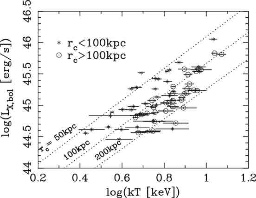
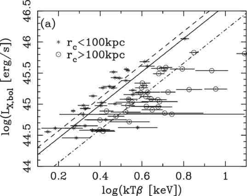
In Fig. 6a, we show the $L_{\rm X}-T$ relation of 69 clusters where we again divide the sample into two subgroups according to two different $r_{c}$ ranges. As pointed out in Ota & Mitsuda (2002), the distributions of the two subgroups are systematically shifted in the figure; the luminosity of a small core cluster is on average higher than that of a large core cluster for a fixed temperature. If we fit all the 69 clusters at the same time, we obtain a power-law index of $3.01^{+0.49}_{-0.44}$ (90% error). Since we found that there is not significant difference in the power-law indices between the two subgroups (Table 1), we obtain the best-fit normalization factors of the relation to be $1.05^{+0.12}_{-0.11}\times 10^{43}~{}{\rm erg\,s^{-1}}$ and $4.52^{+0.37}_{-0.34}\times 10^{42}~{}{\rm erg\,s^{-1}}$ by fitting them separately but fixing the indices at the mean value of 3.01. Thus the difference is significant: the cluster with a smaller core radius is in general brighter for a given temperature. The fitting results are summarized in Table 1.

4.2 $L_{\rm X}-T-r_{c}$ Relation

The above observational results show that the dispersion around the mean $L_{\rm X}-T$ relation is connected with the cluster core size. Assuming the best-fit power-law index of $\alpha=3.01$, we scale the luminosity of each cluster to the luminosity for temperature of 1 keV as $L_{\rm 1keV}=L_{\rm X}(kT/1{\rm keV})^{-\alpha}$. In Fig. 6b, we plot $L_{\rm 1keV}$ as a function of $r_{c}$. We found that there is a negative correlation approximated as $L_{\rm 1keV}\propto r_{c}^{-1.01^{+0.17}_{-0.21}}$ from the fitting. This suggests that $L_{\rm X}$ depends not only on $T$ but on $r_{c}$ as

$$L_{\rm X}\propto T^{3.0}{r_{c}}^{-1}.$$ (14)

The result is consistent with that derived by Fabian et al. (1994), although they interpreted the dependence on $r_{c}$ as the cooling-flow rate. Moreover, Eq. 14 is also consistent with the X-ray fundamental plane of nearby clusters noted by Fujita & Takahara (1999). In the next subsection, we will derive a simple model for the $L_{\rm X}-T$ relation under the assumption of $\beta$-model, incorporating the two characteristic core radii, and compare with the observation.

4.3 Comparison to a $L_{\rm X}-T-r_{c}$ Model

We obtained the following observational facts so far: 1) $r_{c}$ distribution shows high concentration at 50 and 200 kpc, which result in a large dispersion of $r_{c}$, 2) $r_{c}$ does not show strong correlation with the virial radius, and 3) $L_{\rm X}$ depends on both $T$ and $r_{c}$. These results suggest that $r_{c}$ is determined by some physical process in the core region of the cluster, independent of the cluster virial mass. We thus modify the assumption of self-similarity and consider its consequence on the $L_{\rm X}-T$ relation.

In order to evaluate the $L_{\rm X}-T$ relation quantitatively, we assume the isothermal $\beta$-model for the gas density and a constant gas-mass fraction. The details of the calculation of this simple “$L_{\rm X}-T-r_{c}$ model” will be mentioned in Appendix A. For a typical value of $\beta=0.7$, we obtain the model in the form of:

$$L_{\rm X}\propto f_{\rm gas}^{2}(\Delta_{c}\rho_{\rm crit})^{-0.05}T_{\rm gas}^{2.6}r_{c}^{-1.1}.$$ (15)

This is close to the observed relation (and the equation for the X-ray fundamental plane, Eq. 14), however, the index for $T_{\rm gas}$ is smaller than the observation. In Fig. 7, we show the model curves for three different values of $r_{c}$. Thus the $L_{\rm X}-T-r_{c}$ model based on the isothermal $\beta$ model may roughly fit the observed trends of the $L_{\rm X}-T$ relation, though not sufficient to reproduce the data quantitatively.

4.4 X-ray Fundamental Plane Analysis

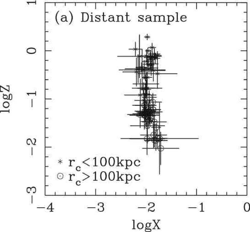
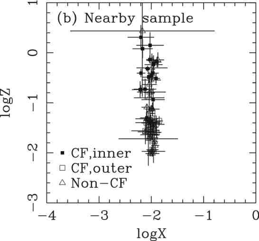
To look further for an essential parameter to understand the dispersion around the $L_{\rm X}-T$ relation, we investigate the X-ray fundamental plane in the $(\log n_{e0},\log T,\log r_{c})$ space for the distant sample. We utilize a method similar to Fujita & Takahara (1999) but carry out a $\chi^{2}$ fit to take into account the statistical errors. As a result, we obtained three orthogonal parameters as follows:

$$X \propto n_{e0}^{0.44}r_{c}^{0.65}T^{-0.62},$$ (16)

$$Y \propto n_{e0}^{0.45}r_{c}^{0.44}T^{0.78},$$ (17)

$$Z \propto n_{e0}^{0.78}r_{c}^{-0.62}T^{-0.10}.$$ (18)

In Fig. 8a, the $\log{X}-\log{Z}$ plane for the distant clusters is shown. We found that the above equations agree with those obtained for the nearby sample by Fujita & Takahara (1999) and then the $z>0.1$ and $z<0.1$ clusters are distributed approximately on the same fundamental plane. In Fig. 8b we also show the distribution of nearby clusters projected onto the same $\log{X}-\log{Z}$ plane, whose $\log{Z}$ range coincides well with that of distant clusters.

As $\chi^{2}/{\rm d.o.f.}=492.1/66$ for the first fit (Eq. 16), however, the constancy of $\log{X}$ i.e. the planarity of the cluster distribution in the 3D space is rejected in the strict sense. Besides the data scatter, this is likely due to the presence of a “break” of the fundamental plane that is seen in Fig. 10b. We will go back to this problem in § 5.2.

By setting $X\sim\mbox{const.}$, Eq. 18 yields

$$Z\propto r_{c}^{-1.78}T^{1.00}\propto n_{e0}^{1.20}T^{-0.69}.$$ (19)

Thus the principal axis of the fundamental plane, $Z$ is suggested to be closely related to $r_{c}$. Since $t_{\rm cool}\propto\sqrt{T}/n_{e0}$, Eq. 19 can be rewritten as

$$Z\propto t_{\rm cool}^{-1.2}.$$ (20)

Since the $Z$-axis represents a direction along which the dispersion of the data points becomes the largest in the parameter correlations, $t_{\rm cool}$ is considered to be a key parameter to control the ICM evolution. Hence we will focus on the effect of gas cooling in the next section.

5 $L_{\rm X}-T$ RELATION AND $t_{\rm cool}$

5.1 Radiative Cooling and Temperature Decrease

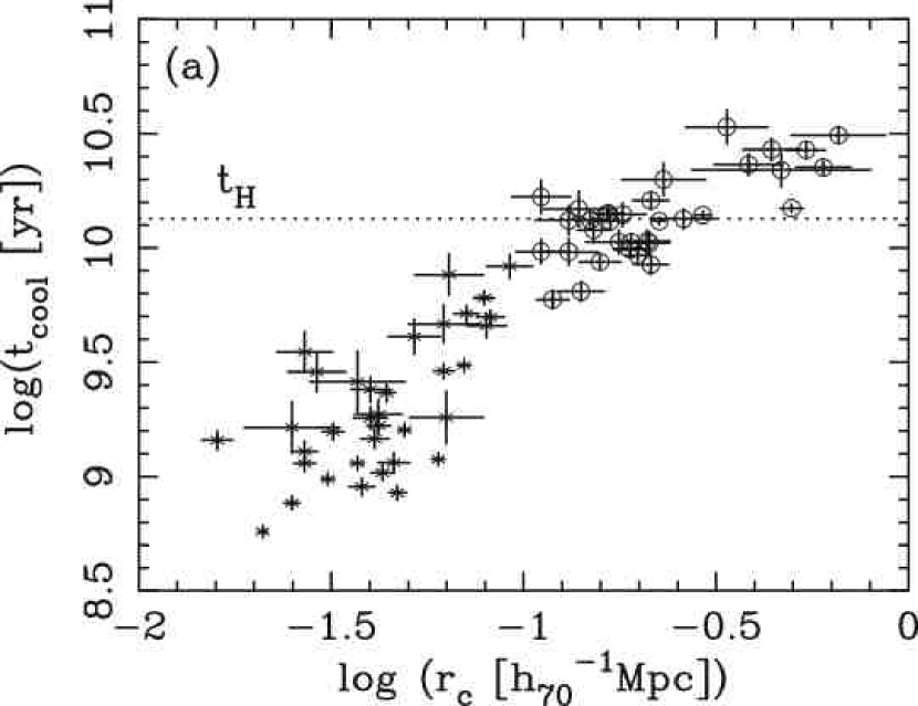
As already mentioned in the previous section, there is a large dispersion of the gas density inside $0.1r_{500}$ region which is strongly related with $r_{c}$ (Fig. 3). Ota & Mitsuda (2004) derived the $n_{e0}-r_{c}$ relation to be $n_{e0}\propto r_{c}^{-1.3}$ and noted that the correlation tends to become even steeper for small core clusters: $n_{e0}\propto r_{c}^{-1.9}$ for $r_{c}<100$ kpc. For clusters with such high density cores, radiative cooling may work considerably. It is also suggestive that $0.1r_{500}$ is roughly equal to the typical cooling radius of $r_{\rm cool}\sim 100$ kpc.

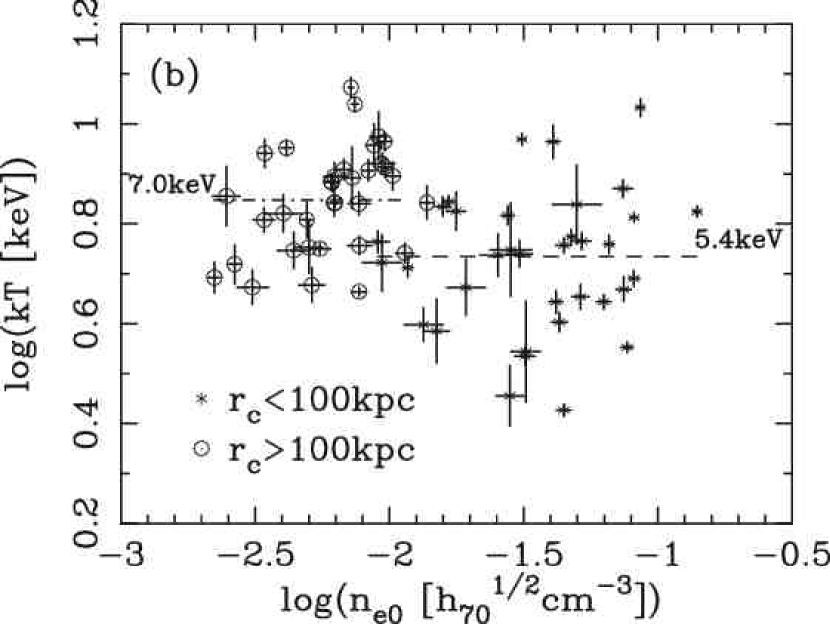
In Fig. 9a we show the radiative cooling time against the core radius. We confirmed that for all small core clusters, it is shorter than the Hubble time ($t_{\rm H}=13.4$ Gyr; Spergel et al. (2003)), $t_{\rm cool}<t_{\rm H}$. Even if we use the age of the Universe at the cluster redshift $t_{\rm age}$ instead of $t_{\rm H}$, which ranges $8.0<t_{\rm age}<12.2$ Gyr for the present sample, that hardly alter the result. Furthermore considering the strong dependence on the core radius, $t_{\rm cool}\propto r_{c}^{1.7}$ for $r_{c}<100$ kpc (Ota & Mitsuda, 2004), these results seem to indicate a central concentration of the gas according to the progress of radiative cooling. This is supportive of an idea of the standard cooling-flow model in this regard. However, as seen from Fig. 9b, there is no clear difference in the temperature range between the two subgroups of different core sizes. The average temperature (and the standard deviation) is 5.4 keV (1.8 keV) for the clusters with $r_{c}<100$ kpc and 7.0 keV (1.8 keV) for $r_{c}>100$ kpc, and the difference is only 30%. Thus there is not a strong temperature drop as predicted by the standard cooling-flow model. Our result confirms the lack of strongly cooled gas based on the large sample of ROSAT and ASCA clusters.

5.2 $L_{\rm X}-T-t_{\rm cool}$ and $L_{\rm X}-T^{\prime}-t_{\rm cool}$ Relations

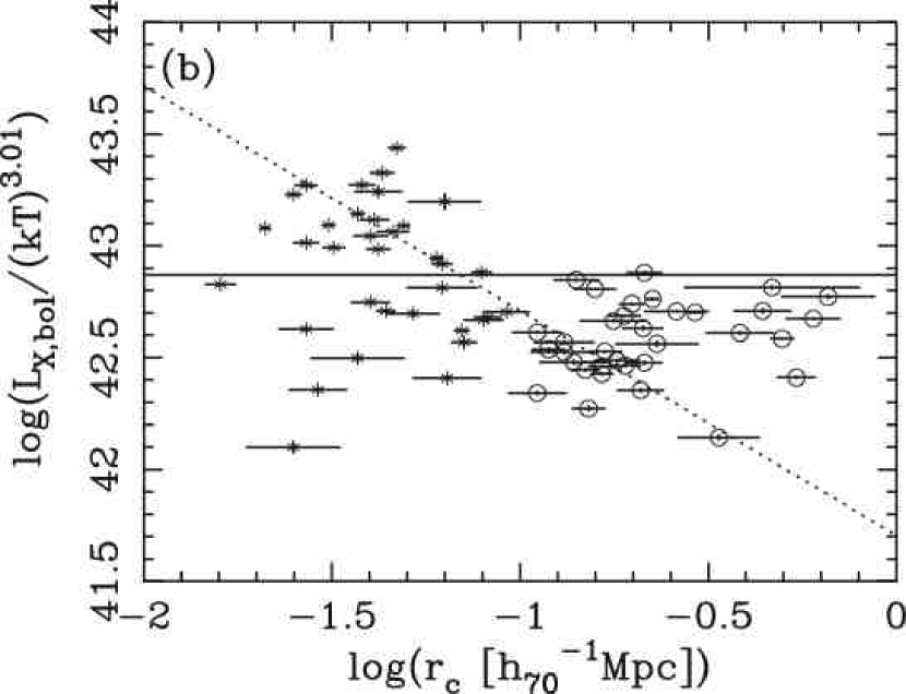
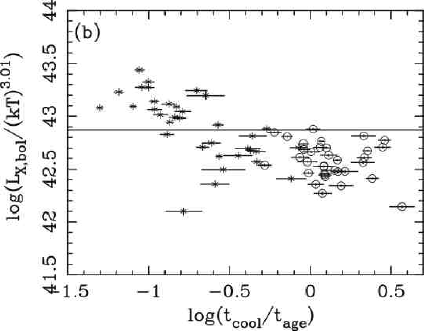
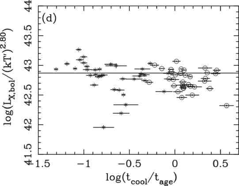
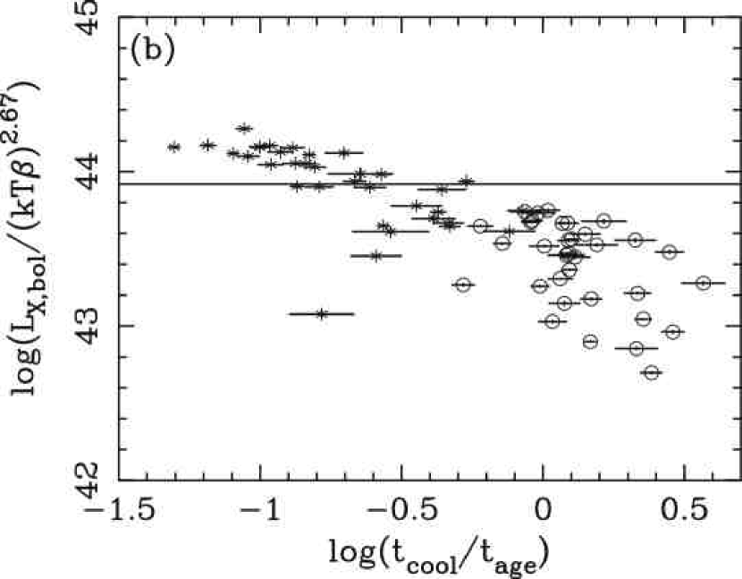
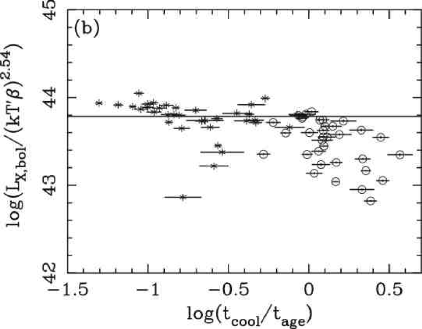
To investigate the nature of the dispersion around the $L_{\rm X}-T$ relation in more detail, we show $L_{\rm 1keV}$ as a function of the cooling time normalized by the age of the universe at the cluster redshift, $(t_{\rm cool}/t_{\rm age})$ in Fig. 10b. At $\log(t_{\rm cool}/t_{\rm age})>-0.5$ the distribution is nearly constant within the data scatter. On the other hand, at the shorter cooling time of $\log(t_{\rm cool}/t_{\rm age})\lesssim-0.5$, a significant deviation from the mean $L_{\rm X}-T$ relation (which is denoted with the horizontal solid line in the figure) is clearly visible. We found that the result depends little on the redshift, as shown in Fig. 11. Although this was interpreted as central excess emission accompanied by the radiative cooling within the framework of the standard cooling-flow model, we want to suggest another possibility that we might underestimate the temperature for the clusters with short cooling time because of mild temperature decrease at the center.

We then evaluate the emission weighted temperature of the clusters with short cooling time utilizing the universal temperature profile found in many nearby cooling-flow clusters. Assuming a projected temperature profile, $T(r)\propto 0.40+0.61[(x/x_{c})^{1.9}/(1+(x/x_{c})^{1.9}]$ ($x=r/r_{2500}$) for relaxed clusters (Allen et al., 2001c) and the $\beta$ profile, $S(r)\propto(1+(r/r_{c})^{2})^{-3\beta+1/2}$, $T=\int^{r_{\rm max}}_{0}T(r)S(r)2\pi rdr/\int^{r_{\rm max}}_{0}S(r)2\pi rdr$ . Since the temperature profile is nearly constant outside the typical cooling radius of $\sim 100$ kpc, we obtain a temperature of the outer, non-cooling region, $T^{\prime}$ to be

$$T^{\prime}\sim 1.3T,$$ (21)

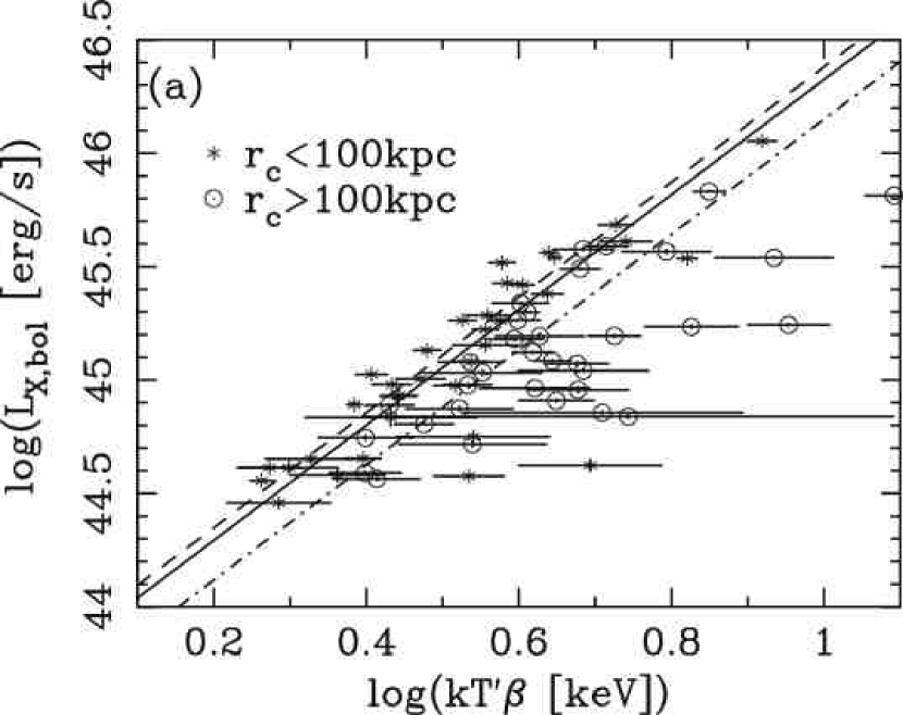
for the typical values of $r_{c}=50$ kpc, $\beta=0.6$, $r_{2500}=600$ kpc and $r_{\rm max}=1$ Mpc. If the temperature starts to decrease again at a larger radius, $r\sim 0.15r_{180}$ as observed in nearby relaxed clusters (e.g. Vikhlinin et al., 2005; Markevitch et al., 1998), it would affect the above equation by only $\lesssim 10$% due to a rapid decrease of the surface brightness at such large radii. Therefore $T$ is likely to underestimate the ambient temperature by about 30% for $t_{\rm cool}\ll t_{\rm age}$. Notice that this estimation is also consistent with the difference of 30% in the average temperature between two subgroups shown in the previous subsection. Thus we consider that it is worth examining the luminosity - “ambient temperature” relation.

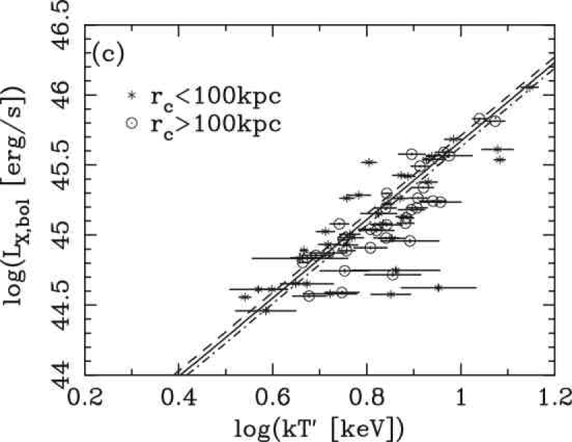
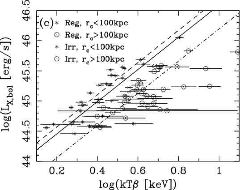
By simply adopting the correction $T^{\prime}=1.3T$ for 26 clusters with $\log(t_{\rm cool}/t_{\rm age})\leq-0.5$ otherwise $T^{\prime}=T$ for 43 clusters, we plot the $L_{\rm X}-T^{\prime}$ relation in Fig. 10c. As listed in Table 1, the difference in the normalization factors between $r\lessgtr 100$ kpc mostly disappeared in this case. The slope of the power-law function is $2.80^{+0.28}_{-0.24}$ and thus marginally less steep compared with that of $L_{\rm X}-T$. Fukazawa et al. (2004) recently derived scaling relations using the ASCA archival data on $\sim 300$ objects over a wide range of mass scales from elliptical galaxies to clusters. They found a smaller index of the $L_{\rm X}-T$ relation, $\alpha=2.34\pm 0.29$ at $kT>4$ keV. Their analysis is different from the present one in that they utilized an integration area extending to 2–3 times $r_{500}$ for luminosity and the area excluding the central $1^{\prime}-3^{\prime}$ region for temperature. Their temperature should therefore be closer to $T^{\prime}$ than $T$. In fact, the index of the $L_{\rm X}-T^{\prime}$ relation mentioned above is slightly larger than but consistent within error bars with the result of Fukazawa et al. (2004).

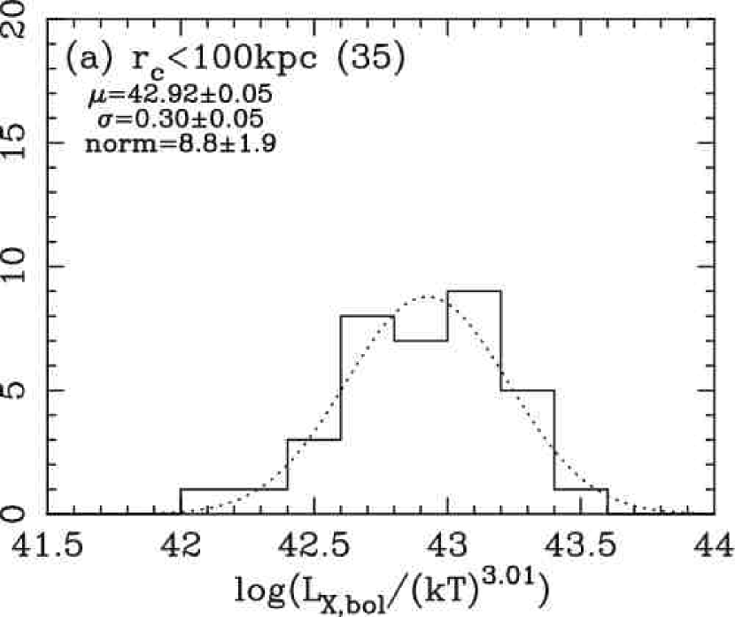
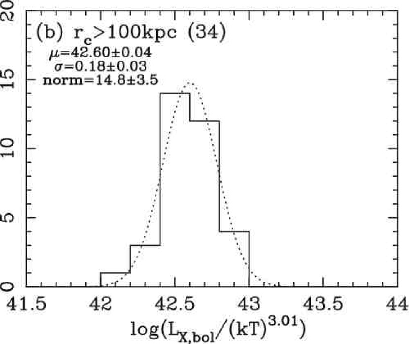
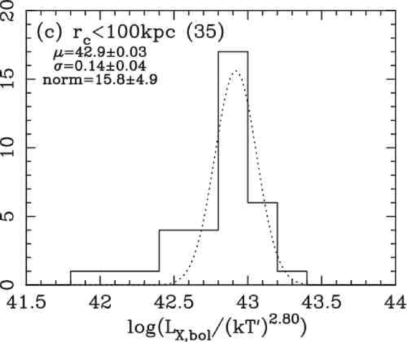
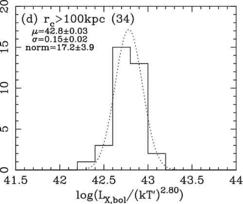
In Fig. 10d we show $L_{\rm 1keV}(=L_{\rm X}/T^{\prime 2.80})$ versus $(t_{\rm cool}/t_{\rm age})$. To quantify the dispersions and demonstrate their changes, we plot histograms of $L_{\rm 1keV}$ for the two $r_{c}$ groups and those with the above correction in Fig. 12. Since we are interested in the statistical significance of the change of the width, we performed the Gaussian fitting with the $\chi^{2}$ method to include the Poisson error of each bin. The resultant Gaussian parameters (the mean, $\mu$ and the width, $\sigma$) and the $1\sigma$ errors are listed in Table 2 and also shown in each panel of Fig. 12. We thus found that by correcting the temperature with Eq. 21, the width significantly decreased from $\sigma/\mu=(7.0\pm 1.2)\times 10^{-3}$ to $(3.3\pm 0.9)\times 10^{-3}$ ($1\sigma$ error) for the smaller $r_{c}$ group (see Fig. 12a, c) and the difference of the widths between two $r_{c}$ groups disappeared: $\sigma/\mu=(3.3\pm 0.9)\times 10^{-3}$ and $(3.5\pm 0.5)\times 10^{-3}$ (Fig. 12c, d). Note that the $1\sigma$ error of $\sigma/\mu$ is dominated by that of $\sigma$ and thus calculated by simply propagating the errors of $\sigma$ and $\mu$.

It is also remarkable that after the correction, there is no significant difference in the dispersions of the data points between $t_{\rm cool}\lessgtr t_{\rm age}$ and $L_{\rm 1keV}$ can be regarded as constant within the data scatter over two orders of magnitudes of $t_{\rm cool}$ (see also Table 2). Thus we consider that this also gives an evidence against the standard cooling-flow model because it predicts cooling that is increasingly enhanced with time. Our result indicates that the luminosity, that is the rate of thermal energy loss by the radiative cooling, does not depend on time very much, and some steady-state is attained for the gas of many small-core clusters. We will discuss about this in more detail in § 7.

6 $L_{\rm X}-T\beta$ RELATION AND X-RAY MORPHOLOGY

6.1 $L_{\rm X}-T\beta$ Relation

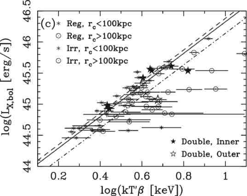
In the case that the intracluster gas follows the isothermal $\beta$-model, the virial temperature should be represented by $T_{\rm vir}=\beta T_{\rm gas}x^{2}(1+x^{2})^{-1}\sim\beta T_{\rm gas}$, where $x\equiv r_{\rm vir}/r_{c}$ and typically $x\gg 1$ (Ota, 2001; Akahori & Masai, 2005). We then replace $T$ with $\beta T$ (here $\beta$ is the slope parameter determined from the ROSAT HRI radial profile fitting) and derive the $L_{\rm X}-T\beta$ correlation (Fig. 13a).

As a result, the power-law index of the $L_{\rm X}-T\beta$ relation is determined to be $2.67\pm 0.44$ , which is marginally smaller in comparison to that of the $L_{\rm X}-T$. As for the data scatter around the mean relation, it becomes smaller for the small-core clusters: the width changes from $\sigma/\mu=(7.0\pm 1.2)\times 10^{-3}$ to $(4.6\pm 0.7)\times 10^{-3}$ from $L_{\rm X}-T$ to $L_{\rm X}-T\beta$, while it becomes marginally larger for the large-core clusters: $(4.2\pm 0.7)\times 10^{-3}$ to $(10.8\pm 7.8)\times 10^{-3}$. The results are also summarized in Tables 1 and 2.

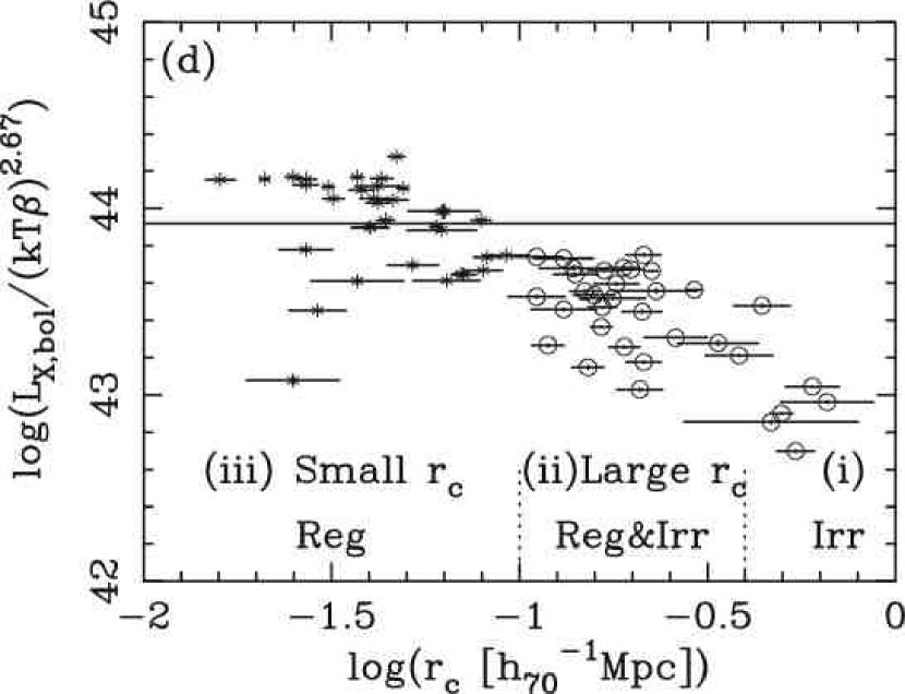
To look into the cause, we investigated parameter correlations, $\beta-T$ and $\beta-r_{c}$. We found that the $\beta-T$ correlation is not significant (the correlation coefficient is 0.24) and at most $\beta\propto T^{0.17^{+0.08}_{-0.09}}$. On the other hand, there is a trend to find larger $r_{c}$ for larger $\beta$ noticeably at $r_{c}>100$ kpc though such a trend is not clear for $r_{c}<100$ kpc. In addition, several clusters show highly inhomogeneous surface brightness distributions and very large cores of $r_{c}>400$ kpc, which form a small peak at around $r_{c}\sim 500$ kpc in the $r_{c}$ histogram (Fig. 5b). Considering that a large fraction of large-core clusters (24 out of 34) exhibit irregular X-ray surface brightness distribution, we may say that the above change in the dispersion likely reflects the X-ray morphology (see § 3.2 and Table 2 of Ota & Mitsuda (2004) for classification of the X-ray morphology).

Particularly, all the five clusters that are located far below the mean relation (i.e. #30 A1895 (catalog ), #50 AC118 (catalog ), #18 MS0451.5+0250 (catalog ), #46 1E0657-56 (catalog ), and #44 A483 (catalog )) have multiple peaks or a signature of cold front in the X-ray images, which can be attributed to cluster merging. In addition, they have very large core radii of $r_{c}\gtrsim 400$ kpc and large $\beta\sim 1$ in comparison to the average value for the distant sample, $\langle\beta\rangle=0.64$ (Ota & Mitsuda, 2004). In Fig. 13b, they appear at the largest end of $r_{c}$. If we exclude the five clusters and estimate the width of the distribution of $L_{\rm 1keV}(=L_{\rm X}/(kT\beta)^{2.67})$, it results in a smaller value of $\sigma/\mu=(6.4\pm 5.5)\times 10^{-3}$ for 29 large core clusters though it is associated with the large statistical uncertainty. To show the relevance to the X-ray morphology in an alternative way, we divide the sample into the regular and irregular clusters and plot them by using different colors in Figs. 13c and d. We roughly see three phases: i) irregular clusters with very large core radius and smaller $L_{\rm 1keV}$ at $\log{r_{c}}>-0.4$, ii) a coexistence of regular and irregular clusters with large core radius at $-1<\log{r_{c}}<-0.4$, and iii) regular small-core clusters with higher $L_{\rm 1keV}$ at $\log{r_{c}}<-1$. Note that for iii), there is only one exception, which is #17 A115 (catalog ), an irregular cluster lying at the smallest $r_{c}$. Therefore we suggest that the above results show a trend that merging clusters particularly in the phase i) segregate from more relaxed clusters on the $L_{\rm X}-T\beta$ plane.

6.2 $L_{\rm X}-T^{\prime}\beta$ Relation

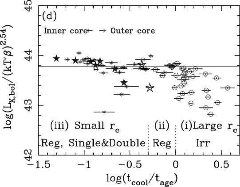
In Fig. 14, we finally show a plot of $L_{\rm X}-T^{\prime}\beta$ relation for $T^{\prime}$ corrected in the same manner as in § 5.2 and Fig. 13. The results of the power-law fitting and the dispersions around the mean relation are also listed in Tables 1 and 2. The power-law index is obtained to be $2.54^{+0.29}_{-0.26}$ from the fitting to 69 clusters. This is smaller in comparison with the $L_{\rm X}-T$ and other three relations derived above, yet significantly steeper than the self-similar model. In Fig. 14b, we find that the distribution of the data points is fairly constant against the cooling time: in particular for 43 clusters with $t_{\rm cool}\leq t_{\rm age}$, the scatter is small: $\sigma/\mu=(2.7\pm 0.5)\times 10^{-3}$ (Table 2). As suggested in the previous subsection, we see again the marginal trend of segregating the merging cluster from the regular clusters in Fig. 14a.

In the next step, we further divide the sample into three subgroups according to the X-ray morphology: the regular single-$\beta$ cluster, the irregular single-$\beta$ cluster, and the regular double-$\beta$ cluster, and distinguish them by using different colors in Fig. 14c and d. From Fig. 14d, we may recognize a trend of the morphological change along the $t_{\rm cool}$ axis. Here it is possible to define three phases as follows: from larger to smaller $t_{\rm cool}$, i) the irregular large-core clusters at $\log(t_{\rm cool}/t_{\rm age})\gtrsim 0$, where a large scatter of $L_{\rm 1keV}$ is seen, ii) the regular large-core clusters at $-0.3\lesssim\log(t_{\rm cool}/t_{\rm age})<0$, and iii) the regular small-core clusters at $\log(t_{\rm cool}/t_{\rm age})<-0.3$. The regular and irregular clusters are no more mixed up in the $L_{\rm 1keV}-t_{\rm cool}$ plot apart from a few exceptions (they are irregular clusters with small $r_{c}$; #17 A115 (catalog ), #38 MS1910+6736 (catalog ), and #11 MS0906.5+1110 (catalog )). It also should be noted that the boundary at $\log{t_{\rm cool}/t_{\rm age}}=0$ in Fig. 14d, i.e. the boundary between i) and ii), approximately corresponds to the crossover point at $\log{t_{\rm cool}}\sim\log{t_{\rm H}}$ and $\log{r_{c}}\sim-0.4$ in Fig. 9a, and thus also to the boundary between i) and ii) in Fig. 13d. Unlike the $L_{\rm 1keV}-r_{c}$ plot (Fig. 13d) where the regular and irregular clusters are mixed in the intermediate range of $r_{c}$, the three groups are now clearly separated from each other in Fig. 14d.

Furthermore, the double-$\beta$ clusters are located in iii) $\log(t_{\rm cool}/t_{\rm age})\lesssim-0.3$, the same region as the regular small-core clusters. As the inner-/outer-core dominant double-$\beta$ clusters are at a shorter/longer side of the range, they are suggested to be closely related to the small-/large-core regular clusters. We thus consider that this may be connected with the evolution of the X-ray surface brightness distribution after the onset of radiative cooling. We will discuss on this point in more detail in the next section.

7 DISCUSSION

7.1 Summary of the Results

From the statistical analysis of 69 distant clusters in $0.1<z<0.56$ with the ROSAT and ASCA X-ray catalog (Ota & Mitsuda, 2004), we have obtained the following observational results.

1. Regarding the cluster outer region, the density profiles are nearly universal and the scatter around the $L_{\rm X}(>0.2r_{500})-T$ relation is surprisingly small. However, the slope of the relation is significantly larger than the self-similar expectation of 2.

2. For the central region, the gas density exhibits a significant scatter and the self-similar condition is not satisfied particularly in the small core clusters.

3. We studied the redshift evolution of the $L_{\rm X}-T$ relation. If restricted the luminosity integration area to the central $0.2r_{500}$ region, there might be a weak, negative evolution, however, the normalization factor of the relation does not significantly change with redshift and is consistent with the nearby sample within the data scatter.

4. We investigated the parameter correlations focusing on the $L_{\rm X}-T$ relation and the connections to $r_{c}$ and $t_{\rm cool}$, and suggested based on the X-ray fundamental plane analysis that $t_{\rm cool}$ is likely to be a control parameter for the ICM structure of the cluster core region.

5. For all small core clusters, $t_{\rm cool}<t_{\rm age}$ and the central electron density is systematically higher as $n_{e0}\propto r_{c}^{-1.9}$, which is suggestive of a central concentration of the gas as cooling progresses. On the other hand, we confirmed that the temperature decrease is mild in the small core clusters; it is estimated as $T=1.3T^{\prime}$ using the universal temperature profile. Then we derived the luminosity-‘ambient temperature’ relation and showed that the dispersion of $L_{\rm 1keV}$ significantly decreases and can be regarded as constant against $t_{\rm cool}$ within the data scatter.

6. From the $L_{\rm X}-T\beta$ and $L_{\rm X}-T^{\prime}\beta$ relations, we showed that $L_{\rm 1keV}$ is related to the X-ray morphology, and that there is a marginal trend for the merging clusters segregating from the regular clusters on their planes. We indicated the possible three phases of the gas property along the $t_{\rm cool}$ axis in Fig. 14d, according to the different level of cooling and ICM density structure.

7.2 Impact of Radiative Cooling on the $L_{\rm X}-T$ Relation and Comparison to the Quasi-hydrostatic Model

In the context of isobaric cooling flow model, the local density of the gas increases against decreasing the temperature so that the thermal pressure $P(r)$ at given $r$ is kept constant within the cooling radius, i.e. $P(r)=n_{e}(r)kT(r)=\mbox{const.}$, and then $n_{e}\propto T^{-1}$ would follow. If this is the case, since $L_{\rm X}\propto n_{e}^{2}T^{1/2}$ for the gas hotter than $kT\sim 2$ keV, the $L_{X}-T$ relation would exhibit $L_{\rm X}\propto T^{-3/2}$. For a typical cooling radius of $r_{\rm cool}\sim 0.1r_{500}$ ($\sim 100$ kpc), $L_{\rm X}(<r_{\rm cool})$ contributes about 50% of the total luminosity. When we derived the $L_{\rm X}(<0.1r_{\rm 500})-T$ relation, however, we did not find any tendency for such an inverse correlation (see also the $L_{\rm X}(<0.2r_{500})-T$ relation in Fig. 4a).

The observational results indicate that the gas in the core region of small core clusters is undergoing radiative cooling but the temperature decline towards the center seems mild. The gas may be considered close to a steady state. We will discuss such a possible state of the gas, quasi-hydrostatic cooling, proposed by Masai & Kitayama (2004). The model predicts a moderate and smooth gas inflow with hydrostatic balancing. In the context, unlike isobaric cooling flows that increase the local density so $P(r)$ is kept against local cooling, quasi-hydrostatic cooling allows the gas to modify its profile or core size so $\nabla P(r)$ matches with the force by gravitational potential.

In § 5.2 we derived the $L_{\rm X}-T^{\prime}$ relation by correcting the emission-weighted temperature for small-core clusters with short $t_{\rm cool}$ based on the idea of the universal temperature profile, and showed that the bolometric luminosity normalized by the temperature dependence of $(kT^{\prime})^{2.8}$, $L_{\rm 1keV}$ is constant within the data scatter over a wide range of $t_{\rm cool}/t_{\rm age}$. This strongly suggests that the rate of thermal energy loss is kept nearly constant after the onset of cooling in the cluster core.

According to the quasi-hydrostatic model, the temperature starts to decrease at the cooling radius and approaches a constant of $\sim 1/3$ the ambient temperature towards the center. The temperature profile does not depend on its absolute value. This picture may explain the observations of nearby cooling-flow clusters. The mass inflow rate from the outer region is controlled by cooling so as to maintain the quasi-hydrostatic balance and is expected to vary little through the flow. The condition is well satisfied in the case that the temperature is $kT\gtrsim 2$ keV where bremsstrahlung dominates cooling more than line emission. The present sample meets this condition since it has a temperature range of $2<kT~{}{\rm[keV]}<12$. Therefore our results can be consistently understood within a framework of the quasi-hydrostatic cooling model.

At the same time, we have found that the gas density profile for the outer part of the cluster does not vary very much from cluster to cluster, and is almost independent of the gas cooling at the center. This would also imply that the energy loss due to radiative cooling at the center is only a portion of the total energy of the thermal gas, and the outer region is likely to offer a great reservoir of the heat, which is carried a fraction into the inner cooling region advectively by the gas inflow under quasi-hydrostatic balance.

As described above, cooling with quasi-hydrostatic balancing modifies the core structure of the gas. This may give a clue to the origin of the small core of $\sim 50$ kpc or the inner core component of the double-$\beta$ cluster. In addition the study would also have an impact on the present understanding of the origin of the dispersions around the $L_{\rm X}-T$ relation because it provided the observational evidence that they are directly linked to the thermal evolution of the ICM and showed how the relation would be modified when the effect of the cooling is considered.

7.3 Evolution of Density Structure of X-ray Clusters

In this subsection we attempt to present an overall picture of the ICM evolution on the basis of the observational results. First we consider about the $r_{c}$ distribution and the origin of the double-$\beta$ nature of the clusters from the phenomenological point of views.

We have reported that the cluster core radius has a large cluster-to-cluster dispersion of more than an order of magnitude, even if restricted the sample to the regular clusters (Ota, 2001). This is partly due to the presence of two peaks separated by a factor of $\sim 4$. For 9 (7) out of the 35 regular clusters, the surface brightness is significantly (marginally) better fitted with the double-$\beta$ model, and the average values of two core radii for the double-$\beta$ clusters coincide well with the two $r_{c}$ peaks of the single-$\beta$ clusters. Then a question may arise: are there three subclasses of clusters, small-core single-$\beta$, large core single-$\beta$, and double-$\beta$ clusters, or are we looking at some different aspects of a single evolutionary process? From the imaging analysis, we noticed that the double-$\beta$ clusters are further subdivided into inner-core dominant and outer-core dominant ones; if we are to perform a single $\beta$ model fitting for these clusters, we would pick up either of the core radii as the best-fit result. Thus the similarity in the $r_{c}$ distributions for the single-$\beta$ and double-$\beta$ clusters can be interpreted in the following way: the (regular) clusters have more or less double-$\beta$ nature in their structure, and when X-ray emission from one of the two cores dominates the whole cluster emission, we recognize it as the single-$\beta$ case and pick up either the inner or outer core as the core radius. This will account for an apparent large dispersion of core radius. Accordingly the single-$\beta$ clusters with a small/large core radius may respectively correspond to extreme cases of inner/outer core dominant double-$\beta$ clusters.

Then why are there inner-core dominant and outer-core dominant clusters? Such double structures have often been attributed to the cooling-flow phenomenon at the cluster center. However, the present analysis showed that the standard cooling-flow model with dynamic inflow is not preferable to account for the results, in particular the $T-n_{e0}$ and $L_{\rm 1keV}-t_{\rm cool}/t_{\rm age}$ relations. On the other hand, in § 6 we suggested the possible three phases of the ICM property on the $L_{\rm 1keV}-t_{\rm cool}/t_{\rm age}$ plane in the light of the radiative cooling and the relevance to a variety of density structure. It is likely that the double-$\beta$ clusters are those in the transient phase of their cooling cores, i.e., core size transition from outer-core dominated to inner-core dominated, mentioned in the quasi-hydrostatic cooling model. As the interpretation of the double core nature, we consider in the following way: when some time passed after the collapse and the cooling becomes important, the core is radiatively cooled and the central density gradually becomes higher to evolve from an outer-core-dominant cluster toward an inner-core-dominant cluster.

The above discussion on the evolution of gas structure focused on the effect of radiative cooling and the possibility of quasi-hydrostatic state since the X-ray analysis showed that a majority of small core clusters are distributed in a narrow range of $L_{\rm 1keV}$ once the temperature bias is corrected (Fig. 12) and thus supports the existence of a typical value. Moreover, a long tail at the smaller $L_{\rm 1keV}$ is seen in the histogram for $r_{c}<100$ kpc (Fig. 12c). This indicates existence of some peculiar clusters or extra physical mechanism that produces such a variation. Recently, O’hara et al. (2005) examined a relation between substructure and cool cores and the scatter about cluster scaling relations using 45 nearby clusters. They found that cool core clusters, which usually have less morphological substructure, exhibit higher intrinsic scatter about scaling relations even after correcting for cooling core effect, suggesting a possibility that a more global process is at work. Then the variation in the $L_{\rm 1keV}$ histogram for the small $r_{c}$ clusters may be related with the scatter found by O’hara et al. (2005). To further clarify both the structural evolution and the scatter of scaling relations, a systematic study with higher sensitivities will be important.

7.4 Related Issues and Future Observations

We will remark on the effect of the cold front detected in nearby clusters with the Chandra observations in regard to the present interpretation, and the assumption of the universal temperature profile with consideration on the recent progress of Chandra and XMM-Newton observations.

The cold front structure is characterized by a compact core with the density and temperature jumps in contrast to the surroundings, and interpreted as a remnant of subcluster merger (Markevitch et al., 2000). For higher redshifts, it is more difficult to directly identify such small structures due to the limitation of the sensitivity to measure the temperature maps, and some of them might possibly be fitted with the double-$\beta$ model. However, as the cold front is a signature of recent merger, it is expected to be accompanied with the irregular X-ray morphology. Thus for relatively bright clusters, a small core of the cold front in an irregular cluster may be distinguishable from that of a regular cluster by referring to the morphological information. For example, A115 (catalog ) and 1E0657-56 (catalog ), for which a possible remnant of cooling core of a merging subcluster was pointed out (Gutierrez & Krawczynski, 2005; Markevitch et al., 2002), were classified into irregular clusters from our image analysis, though they have different $r_{c}$ and are located in the different phases in Fig. 14d ( i) and iii), respectively). For more accurate identification of the cold front in distant clusters, it is necessary to measure the 2 dimensional density and temperature maps with higher sensitivity observations.

We have utilized the universal temperature profile to estimate the effect of temperature decrease and relate the emission-weighted temperature to the ambient temperature for clusters with short cooling time and apparent luminosity enhancement in Fig. 10b. Due to the limited spatial resolution of ASCA, the temperature profiles were not directly constrained for the distant sample. However for some of them, the results have been already published with the Chandra and XMM-Newton data. As for the double-$\beta$ clusters or the small core cluster with very short cooling time of $-1.3\lesssim\log{(t_{\rm cool}/t_{\rm age})}\lesssim-0.7$, A2204 (catalog ), PKS0745-191 (catalog ), A2390 (catalog ), A1835 (catalog ), the gradual temperature decline within the central region of roughly $r<100-200$ kpc were reported (Sanders et al., 2005; Hicks et al., 2002; Allen et al., 2001b; Majerowicz et al., 2002). For the other double-$\beta$ cluster, A1689, with slightly longer $\log{t_{\rm cool}/t_{\rm age}}=-0.56$, the nearly isothermal profile was found with Chandra (Xue & Wu, 2002), and a complex temperature structure was further reported with XMM-Newton (Andersson & Madejski, 2004). Therefore, from the overall standpoint, the assumption of the universal temperature profile for $\log{t_{\rm cool}/t_{\rm age}}\lesssim-0.5$ seems reasonable for many of the small core and double-$\beta$ clusters. To directly confirm the temperature structure in relation to the gas cooling, we need to analyze the temperature profile of individual clusters in various phases with using higher resolutions.

In § 3.3, we derived the $L_{\rm X}(>0.2r_{500})-T$ relation without correcting for the temperature profile. Adopting the corrected temperature $T^{\prime}=1.3T$ (Eq. 21), we obtain a similar slope, $L_{\rm X}(>0.2r_{500})=2.34^{+2.35}_{-1.13}\times 10^{42}(kT^{\prime})^{3.05^{+0.33}_{-0.35}}$ for 69 clusters ($\chi^{2}/{\rm d.o.f.}=610/67$) (Table 1) and a smaller standard deviation for $L_{\rm 1keV}$, $\sigma/\mu=(4.5\pm 0.5)\times 10^{-3}$. Once the ambient temperature $T^{\prime}$ is directly measured for a large sample of clusters by future observations, we would suggest to use it instead of $T$ in the analysis of cluster scaling relations.

Appendix A A SIMPLE $L_{\rm X}-T-r_{c}$ MODEL

In order to evaluate the $L_{\rm X}-T$ relation quantitatively, we assume the $\beta$ profile for the gas density;

$$\rho_{\rm gas}=\rho_{\rm gas,0}\left[1+\left(\frac{r}{r_{c}}\right)^{2}\right]^{-3\beta/2}.$$ (A1)

Then the total gas mass, $M_{\rm gas}$, within $r_{\rm vir}$ is evaluated by

$$M_{\rm gas}=4\pi r_{c}^{3}\rho_{\rm gas,0}\int_{0}^{x_{\rm v}}x^{2}(1+x^{2})^{-3\beta/2}dx,$$ (A2)

where $x_{\rm v}=r_{\rm vir}/r_{c}$. For the observed range of $x_{\rm v}$, i.e. $4<x_{\rm v}<64$ (see Fig. 1), the integral in Eq. A2 can be well approximated by a single power law function, thus is $\propto x_{\rm v}^{a}$ for a fixed value of $\beta$ (Evrard & Henry, 1991). Under the assumptions that the cluster mean density is $\Delta_{c}$ times the critical density of the universe, $\bar{\rho}=3M_{\rm vir}/4\pi r_{\rm vir}^{3}=\Delta_{c}\rho_{\rm crit}$, and the gas-mass fraction, $f_{\rm gas}=M_{\rm gas}/M_{\rm vir}$ is constant among clusters, Eq. A2 yields

$$M_{\rm gas}\simeq\frac{4\pi}{3}r_{\rm vir}^{3}\Delta_{c}\rho_{\rm crit}f_{\rm gas}.$$ (A3)

Eqs. A2 and A3 relate the central gas density, $\rho_{\rm gas,0}$, with $r_{c}$ and $r_{\rm vir}$ as follows.

$$\rho_{\rm gas,0}=\frac{1}{3}x_{\rm v}^{3-a}\Delta_{c}\rho_{\rm crit}f_{\rm gas}.$$ (A4)

The X-ray luminosity, $L_{\rm X}$, is expressed as

$$L_{\rm X} = \Lambda(T_{\rm gas})4\pi r_{c}^{3}\left(\frac{\rho_{\rm gas,0}}{\bar{m}}\right)^{2}\int^{x_{\rm v}}_{0}x^{2}(1+x^{2})^{-3\beta}dx,$$ (A5)

$$\simeq \Lambda(T_{\rm gas})4\pi r_{c}^{3}\left(\frac{\rho_{\rm gas,0}}{\bar{m}}\right)^{2}x_{\rm v}^{b},$$ (A6)

$$\simeq 1.435\times 10^{-27}\frac{4\pi}{9\bar{m}^{2}}\left(\frac{9\beta k}{4\pi\bar{m}G}\right)^{3-a+b/2}$$ (A8)

$$\cdot f_{\rm gas}^{2}(\Delta_{c}\rho_{\rm crit})^{-1+a-b/2}T_{\rm gas}^{7/2-a+b/2}r_{c}^{-3+2a-b},$$

where $\Lambda$ is the emissivity of the free-free emission and $\bar{m}=\mu m_{p}$ ($\mu$ : the mean plasma weight, 0.63). In the case of $\beta=0.7$, $a=0.96$, and $b=0.025$ for $x_{\rm v}=32$ ($x_{\rm v}$ dependence is small), which leads

$$L_{\rm X}\propto f_{\rm gas}^{2}(\Delta_{c}\rho_{\rm crit})^{-0.05}T_{\rm gas}^{2.6}r_{c}^{-1.1}.$$ (A9)

We define the virial temperature as

$$kT_{\rm vir}\equiv\frac{\bar{m}GM_{\rm vir}}{3r_{\rm vir}}=\frac{4\pi\bar{m}G\Delta_{c}\rho_{\rm crit}r_{\rm vir}^{2}}{9},$$ (A10)

and assume that it is related to the gas temperature through $kT_{\rm vir}\equiv\beta^{\prime}kT_{\rm gas}$.

In Fig. 7, we show the $L_{\rm X}-T$ relation numerically calculated according to Eq. A8 for $r_{c}=50,100,200~{}h_{70}^{-1}{\rm kpc}$, $\beta=0.7$, and $\Delta_{c}=500$. The gas-mass fraction within $r_{\rm vir}(=r_{\rm 500})$ is fixed at the mean value of $f_{\rm gas}=0.27$ for the distant sample (Ota & Mitsuda, 2004). We should notice that dependence of $L_{\rm X}-T$ relation on $\rho_{\rm crit}\Delta_{c}$ is very small; the power-law index is $-0.05$, and is almost independent of the cluster-collapse epoch. Then the collapse redshift is assumed to be $z_{\rm col}=0.3$, which is an average observed redshfit of the sample. We adjusted the value of $\beta^{\prime}$ to $\beta^{\prime}=0.4\beta$ in the calculation so as to make the absolute values of $L_{\rm X}$ consistent with the observations.

Figure 1: (a) Comparison of two luminosity measurements. The bolometric luminosities within $r_{500}$ estimated from the ROSAT HRI are plotted against those from the ASCA GIS. The clusters are divided into three subgroups according to the best-fit temperature from the ASCA spectroscopy, 18 clusters with $2<kT~{}{\rm[keV]}<5$, 30 clusters with $5<kT~{}{\rm[keV]}<7$ and 21 clusters with $7<kT~{}{\rm[keV]}<12$ and denoted with the crosses, the asterisks, and the open circles, respectively. The solid line corresponds to $L_{\rm X,HRI}=L_{\rm X,GIS}$. (b) Comparison of the cooling time, $t_{\rm cool}$ estimated with the ROSAT and ASCA analysis (Ota & Mitsuda, 2004) and Chandra (Bauer et al., 2005) regarding 21 clusters with $0.15<z<0.35$.

Figure 2: $r_{500}-r_{c}$ relation (a) and histogram of $r_{c}$ (b) for 69 clusters. In the panel (a), 35 clusters with small core of $r_{c}<100$ kpc and 34 clusters with larger core of $r_{c}>100$ kpc are shown with the green asterisks and the magenta circles, respectively. The dotted lines indicate the self-similar condition corresponding to four different constant values of $r_{500}/r_{c}$.

Figure 3: Electron density profiles for 69 clusters. The best-fit density profiles derived with the single $\beta$-model are plotted, where the radius is normalized with $r_{500}$. $0.1r_{500}$ is indicated with the vertical dotted line, inside which the scatter is the most prominent.

Figure 4: $L_{\rm X}(<0.2r_{500})-T$ relation (a) and $L_{\rm X}(>0.2r_{500})-T$ relation (b). The sample is divided into two $r_{c}$ groups and thus the meaning of the symbols are the same as Fig. 2. The solid line represent the best-fit power-law for 69 clusters in each panel. The best-fit models obtained for $r_{c}<100$ kpc and $>100$ kpc are also shown with the dashed and dot-dash lines, respectively.

Figure 5: $L_{\rm X}-T$ relations for three subsets of the data: 18 clusters with $0.1<z<0.2$ (blue crosses), 27 clusters with $0.2<z<0.3$ (green asterisks), and 24 clusters with $0.3<z<0.56$ (red circles). In the panels (a) and (b), the luminosity was calculated within the overdensity radius $r_{500}$. The solid line shows the best-fit power-law model for 69 distant clusters. In the panels (c) and (d), the $L_{\rm X}(<0.2r_{500})-T$ and $L_{\rm X}(>0.2r_{500})-T$ relations are shown, respectively. In the panels (e) and (f), the luminosity was calculated for a fixed radius of 2 Mpc. For 26 clusters with a short cooling time, we corrected the effect of possible cool emission regarding both the luminosity and temperature (see text for details). The solid line indicates the local relation obtained by Markevitch (1998). In the panel (f), the luminosity was further scaled with redshift as $L_{\rm X}(1+z)^{-1.5}$. In each panel, the blue, green, and red dashed lines show the best-fit power-laws for the above three redshift ranges, respectively. In the panel (a), the slope of the relation was included as a free parameter in the fits, while in the panels (b)–(f), the slope was fixed at $\alpha=3.01$, $4.37$, $2.85$, $2.64$, and $2.64$, respectively.

Figure 6: $L_{\rm X}-T$ relation (a) and $L_{\rm 1keV}-r_{c}$ relation (b). In the panel (a), we find the smaller core clusters are brighter on average compared to the large core ones of the same temperature. In the panel (b), $L_{\rm 1keV}(=L_{\rm X}/(kT)^{3.01})$ is the normalization factor of the $L_{\rm X}-T$ relation derived for each cluster. The solid line indicates the best-fit normalization factor of the $L_{\rm X}-T$ relation for 69 clusters in the panel (b). The negative correlation between $L_{\rm 1keV}$ and $r_{c}$ corresponds to the luminosity difference between the two subgroups, which is roughly approximated as $L_{\rm 1keV}\propto r_{c}^{-1}$ (the dotted line).

Figure 7: $L_{\rm X}-T$ relations expected for clusters with a constant core radius, $r_{c}=50$ or 100 or 200 kpc (dotted lines). $\beta=0.7$ is assumed in the model calculation. See Appendix A for details of the model.

Figure 8: Results of X-ray fundamental plane analysis. In panel (a), the best-fit $\log{X}-\log{Z}$ plane obtained for the distant clusters is shown. The meaning of the symbols are the same as Fig. 2. In the panel (b), 45 nearby clusters taken from Mohr, Mathiesen & Evrard (1999) were projected onto the same fundamental plane as panel (a). According to Table 2 of Mohr, Mathiesen & Evrard (1999) non cooling-flow clusters are shown with the red triangles, and inner-core and outer-core components of cooling-flow clusters are separately shown with the solid blue boxes and open black boxes.

Figure 9: $t_{\rm cool}-r_{c}$ (a) and $T-n_{e0}$ (b) relations. For panel (a), $t_{\rm cool}$ is the radiative cooling timescale (see text). There is a strong correlation with $r_{c}$ which follows $t_{\rm cool}\propto r_{c}^{1.7}$. The Hubble time, $t_{\rm H}=13.4$ Gyr (Spergel et al., 2003) is indicated with the horizontal dotted line. Then $t_{\rm cool}<t_{\rm H}$ for all clusters belonging to the smaller core group. For panel (b), $n_{e0}$ is the central electron density obtained from the $\beta$ model analysis. There is no clear difference in the temperature range between the two subgroups though $n_{e0}$ is scattered nearly over two orders of magnitudes. Their average temperatures of 5.4 keV and 7.0 keV are shown with the dashed line and dot-dash line, respectively.

Figure 10: $L_{\rm X}-T$ relation and $t_{\rm cool}$. Upper panels, $L_{\rm X}-T$ relation of clusters (a) (the same as Fig. 6a), and $L_{\rm 1keV}$ as a function of $t_{\rm cool}/t_{\rm age}$ (b). Bottom panels, the luminosity to the ‘ambient temperature’ relation, $L_{\rm X}-T^{\prime}$ (c) and $L_{\rm 1keV}=L_{\rm X}/(kT^{\prime})^{2.80}$ as a function of $t_{\rm cool}/t_{\rm age}$ (d). In the panels (c) and (d), for clusters with short cooling timescale of $\log{t_{\rm cool}/t_{\rm age}}<-0.5$, the temperature decrease is corrected with $T^{\prime}=1.3T$, otherwise $T^{\prime}=T$ (see § 5.2). We find a decrease of the dispersion around the mean $L_{\rm X}-T^{\prime}$ relation in comparison to the $L_{\rm X}-T$, which we show in a more quantitative manner in Fig. 12.

Figure 11: $L_{\rm 1keV}$ as a function of $t_{\rm cool}/t_{\rm age}$ in three redshift ranges. In the panels (a) and (b), $L_{\rm 1keV}=L_{\rm X}/(kT)^{3.01}$ (§ 5.2) and $L_{\rm X}/(kT^{\prime}\beta)^{2.54}$ (§ 6.2) are plotted, respectively.

Figure 12: Histograms of $L_{\rm 1keV}$. The distributions of $L_{\rm 1keV}(=L_{\rm X}/(kT)^{3.01})$ for 35 small core clusters and 34 large core clusters are shown with the green and magenta stepped lines in the panels (a) and (b), respectively. The results of $L_{\rm 1keV}(=L_{\rm X}/(kT^{\prime})^{2.80})$ are shown in the panels (c) and (d). The best-fit Gaussian model is shown with the dotted curve in each panel. The Poisson error of each bin was considered in the fitting though it is not displayed in the panels. The fitting results are summarized in Table 2.

Figure 13: $L_{\rm X}-T\beta$ relation and X-ray morphology. Upper panels, $L_{\rm X}-T\beta$ relation of clusters (a) and $L_{\rm 1keV}=L_{\rm X}/(kT\beta)^{2.67}$ as a function of $t_{\rm cool}/t_{\rm age}$ (b). Bottom panels, the same as panel (a) (c), and $L_{\rm 1keV}$ as a function of $r_{c}$ (d). The meaning of the symbols for two $r_{c}$ classes are the same as (a) and (b), but the regular and irregular clusters are shown in blue and red respectively. In the panel (d), we indicated the three phases corresponding to i) the irregular clusters with a very large $r_{c}$ and a signature of merger, ii) the coexistence of the regular and irregular clusters with a large $r_{c}$, and iii) the regular clusters with a small $r_{c}$ (see § 6.1).

Figure 14: $L_{\rm X}-T^{\prime}\beta$ relation and X-ray morphology. The double-$\beta$ clusters are denoted with the light-blue stars. The filled (open) stars correspond to the inner-core (outer-core) dominant double-$\beta$ clusters. In the panel (d), we indicated the three phases according to the different level of cooling and density structure: i) the large core, irregular clusters with long $t_{\rm cool}$ relative to $t_{\rm age}$, ii) the large core, regular clusters with moderate $t_{\rm cool}$, and iii) the small core, regular clusters with short $t_{\rm cool}$. In the phase iii), 9 of the sample shows the significant double-$\beta$ structure, and the inner-core/outer-core dominant double-$\beta$ clusters are located at the shorter/longer cooling time (see § 6.2).

Table 1: X-ray luminosity-temperature relations for the distant sample.

	Sample	Relation	$\chi^{2}/{\rm d.o.f.}\tablenotemark{b}$
$L_{\rm X}-T$	all (69)	$7.41^{+8.89}_{-4.40}\times 10^{42}(kT)^{3.01^{+0.49}_{-0.44}}$	1603/67
	$r_{c}\leq 0.1$ Mpc (35)	$1.05^{+0.12}_{-0.11}\times 10^{43}(kT)^{3.01}$	722/34
	$r_{c}>0.1$ Mpc (34)	$4.52^{+0.37}_{-0.34}\times 10^{42}(kT)^{3.01}$	172/33
	$r_{c}\leq 0.1$ Mpc (35)	$1.45^{+1.62}_{-0.89}\times 10^{43}(kT)^{2.82^{+0.56}_{-0.44}}$	716/33
	$r_{c}>0.1$ Mpc (34)	$4.37^{+4.84}_{-2.30}\times 10^{42}(kT)^{3.03^{+0.38}_{-0.38}}$	172/32
$L_{\rm X}-T^{\prime}$	all (69)	$7.41^{+4.49}_{-3.12}\times 10^{42}(kT^{\prime})^{2.80^{+0.28}_{-0.24}}$	669/67
	$r_{c}\leq 0.1$ Mpc (35)	$8.04^{+0.71}_{-0.65}\times 10^{42}(kT^{\prime})^{2.80}$	461/34
	$r_{c}>0.1$ Mpc (34)	$6.76^{+0.56}_{-0.35}\times 10^{42}(kT^{\prime})^{2.80}$	177/33
	$r_{c}\leq 0.1$ Mpc (35)	$1.04^{+0.85}_{-0.54}\times 10^{43}(kT^{\prime})^{2.67^{+0.37}_{-0.32}}$	457/33
	$r_{c}>0.1$ Mpc (34)	$4.37^{+4.84}_{-2.30}\times 10^{42}(kT^{\prime})^{3.03^{+0.38}_{-0.38}}$	171/32
$L_{\rm X}-T\beta$	all (69)	$8.32^{+5.52}_{-3.32}\times 10^{43}(kT\beta)^{2.67^{+0.44}_{-0.44}}$	1310/67
	$r_{c}\leq 0.1$ Mpc (35)	$1.08^{+0.09}_{-0.12}\times 10^{44}(kT\beta)^{2.67}$	420/34
	$r_{c}>0.1$ Mpc (34)	$3.35^{+0.47}_{-0.49}\times 10^{43}(kT\beta)^{2.67}$	169/33
	$r_{c}\leq 0.1$ Mpc (35)	$1.10^{+0.49}_{-0.40}\times 10^{44}(kT\beta)^{2.66^{+0.41}_{-0.36}}$	420/33
	$r_{c}>0.1$ Mpc (34)	$2.85^{+3.62}_{-1.78}\times 10^{43}(kT\beta)^{2.77^{+0.65}_{-0.54}}$	169/32
$L_{\rm X}-T^{\prime}\beta$	all (69)	$6.10^{+2.57}_{-1.96}\times 10^{43}(kT^{\prime}\beta)^{2.54^{+0.29}_{-0.26}}$	628/67
	$r_{c}\leq 0.1$ Mpc (35)	$6.92^{+0.48}_{-0.67}\times 10^{43}(kT^{\prime}\beta)^{2.54}$	294/34
	$r_{c}>0.1$ Mpc (34)	$4.03^{+0.56}_{-0.40}\times 10^{43}(kT^{\prime}\beta)^{2.54}$	172/33
	$r_{c}\leq 0.1$ Mpc (35)	$7.16^{+3.29}_{-2.25}\times 10^{43}(kT^{\prime}\beta)^{2.51^{+0.30}_{-0.28}}$	293/33
	$r_{c}>0.1$ Mpc (34)	$2.85^{+3.62}_{-1.78}\times 10^{43}(kT^{\prime}\beta)^{2.77^{+0.65}_{-0.54}}$	169/32
$L_{\rm X}(<0.2r_{500})-T$	all (69)	$3.02^{+45.22}_{-2.83}\times 10^{41}(kT)^{4.37^{+1.54}_{-1.50}}$	2995/67
	$r_{c}\leq 0.1$ Mpc (35)	$5.82^{+1.91}_{-1.12}\times 10^{41}(kT)^{4.37}$	1289/34
	$r_{c}>0.1$ Mpc (34)	$8.32^{+1.58}_{-1.57}\times 10^{40}(kT)^{4.37}$	301/33
	$r_{c}\leq 0.1$ Mpc (35)	$2.88^{+12.70}_{-2.35}\times 10^{42}(kT)^{3.43^{+0.98}_{-0.98}}$	1231/33
	$r_{c}>0.1$ Mpc (34)	$9.23^{+20.29}_{-6.77}\times 10^{41}(kT)^{3.13^{+0.67}_{-0.59}}$	252/32
$L_{\rm X}(>0.2r_{500})-T$	all (69)	$4.95^{+3.45}_{-2.13}\times 10^{42}(kT)^{2.85^{+0.30}_{-0.27}}$	551/67
	$r_{c}\leq 0.1$ Mpc (35)	$5.56^{+0.62}_{-0.56}\times 10^{42}(kT)^{2.85}$	321/34
	$r_{c}>0.1$ Mpc (34)	$4.27^{+0.48}_{-0.32}\times 10^{42}(kT)^{2.85}$	174/33
	$r_{c}\leq 0.1$ Mpc (35)	$7.41^{+7.19}_{-3.91}\times 10^{42}(kT)^{2.68^{+0.43}_{-0.37}}$	317/33
	$r_{c}>0.1$ Mpc (34)	$1.45^{+1.75}_{-0.90}\times 10^{42}(kT)^{3.40^{+0.48}_{-0.40}}$	148/32
$L_{\rm X}(>0.2r_{500})-T^{\prime}$	all (69)	$2.34^{+2.35}_{-1.13}\times 10^{42}(kT^{\prime})^{3.05^{+0.33}_{-0.35}}$	610/67
	$r_{c}\leq 0.1$ Mpc (35)	$2.04^{+0.26}_{-0.24}\times 10^{42}(kT^{\prime})^{3.05}$	362/34
	$r_{c}>0.1$ Mpc (34)	$2.88^{+0.29}_{-0.26}\times 10^{42}(kT^{\prime})^{3.05}$	158/33
	$r_{c}\leq 0.1$ Mpc (35)	$5.07^{+5.89}_{-2.97}\times 10^{42}(kT^{\prime})^{2.59^{+0.45}_{-0.38}}$	336/33
	$r_{c}>0.1$ Mpc (34)	$1.45^{+1.75}_{-0.59}\times 10^{42}(kT^{\prime})^{3.40^{+0.22}_{-0.40}}$	148/33

Table 2: Means and standard deviations of $\log{L_{\rm 1keV}}$.

$\log{L_{\rm 1keV}}$	Sample	$\mu$	$\sigma$	$\chi^{2}/{\rm d.o.f.}\tablenotemark{b}$	$\sigma/\mu~{}[10^{-3}]$
$\log{L_{\rm X}/(kT)^{3.01}}$	all (69)	$42.75\pm 0.04$	$0.31\pm 0.04$	4.73/5	$7.3\pm 0.9$
	$r_{c}\leq 0.1$ Mpc (35)	$42.92\pm 0.05$	$0.30\pm 0.05$	1.95/5	$7.0\pm 1.2$
	$r_{c}>0.1$ Mpc (34)	$42.60\pm 0.04$	$0.18\pm 0.03$	0.82/2	$4.2\pm 0.7$
	$t_{\rm cool}\leq t_{\rm age}$ (43)	$42.88\pm 0.05$	$0.30\pm 0.04$	2.07/5	$7.0\pm 0.9$
	$t_{\rm cool}>t_{\rm age}$ (26)	$42.57\pm 0.04$	$0.18\pm 0.04$	0.56/2	$4.2\pm 0.9$
$\log{L_{\rm X}/(kT^{\prime})^{2.80}}$	all (69)	$42.82\pm 0.03$	$0.19\pm 0.02$	4.53/5	$4.4\pm 0.5$
	$r_{c}\leq 0.1$ Mpc (35)	$42.92\pm 0.03$	$0.14\pm 0.04$	7.35/5	$3.3\pm 0.9$
	$r_{c}>0.1$ Mpc (34)	$42.78\pm 0.03$	$0.15\pm 0.02$	0.78/2	$3.5\pm 0.5$
	$t_{\rm cool}\leq t_{\rm age}$ (43)	$42.87\pm 0.04$	$0.19\pm 0.04$	5.23/5	$4.4\pm 0.9$
	$t_{\rm cool}>t_{\rm age}$ (26)	$42.77\pm 0.04$	$0.16\pm 0.03$	0.99/2	$3.7\pm 0.7$
$\log{L_{\rm X}/(kT\beta)^{2.67}}$	all (69)	$43.63\pm 0.05$	$0.35\pm 0.05$	11.53/6	$8.0\pm 1.1$
	$r_{c}\leq 0.1$ Mpc (35)	$43.92\pm 0.04$	$0.20\pm 0.02$	7.67/3	$4.6\pm 0.7$
	$r_{c}>0.1$ Mpc (34)	$43.69\pm 0.76$	$0.47\pm 0.34$	0.75/3	$10.8\pm 7.8$
	$t_{\rm cool}\leq t_{\rm age}$ (43)	$43.86\pm 0.04$	$0.22\pm 0.03$	11.22/4	$5.0\pm 0.7$
	$t_{\rm cool}>t_{\rm age}$ (26)	$43.44\pm 0.27$	$0.41\pm 0.20$	2.62/3	$9.4\pm 4.6$
$\log{L_{\rm X}/(kT^{\prime}\beta)^{2.54}}$	all (69)	$43.60\pm 0.27$	$0.26\pm 0.20$	18.98/4	$6.0\pm 4.6$
	$r_{c}\leq 0.1$ Mpc (35)	$43.83\pm 0.02$	$0.11\pm 0.02$	3.58/3	$2.5\pm 0.5$
	$r_{c}>0.1$ Mpc (34)	$43.81\pm 0.02$	$0.29\pm 0.06$	2.66/3	$6.7\pm 1.4$
	$t_{\rm cool}\leq t_{\rm age}$ (43)	$43.81\pm 0.02$	$0.12\pm 0.02$	5.92/3	$2.7\pm 0.5$
	$t_{\rm cool}>t_{\rm age}$ (26)	$43.41\pm 0.07$	$0.29\pm 0.07$	2.13/3	$6.7\pm 1.6$

References

- Akahori & Masai (2005) Akahori, T. & Masai, K. 2005, PASJ, 57, 419
- Allen & Fabian (1998) Allen, S. W., & Fabian, A. C. 1998, MNRAS, 297, L57
- Allen et al. (2001a) Allen, S. W., et al. 2001a, MNRAS, 324, 842
- Allen et al. (2001b) Allen, S. W., Ettori, S., & Fabian, A. C. 2001b, MNRAS, 324, 877
- Allen et al. (2001c) Allen, S. W., Schmidt, R. W., & Fabian, A. C. 2001, MNRAS, 328, L37
- Andersson & Madejski (2004) Andersson, K. E., & Madejski, G. M. 2004, ApJ, 607, 190
- Arnaud & Evrard (1999) Arnaud, M., & Evrard, A. E. 1999, MNRAS, 305, 631
- Bauer et al. (2005) Bauer, F. E., Fabian, A. C., Sanders, J. S., Allen, S. W., & Johnstone, R. M. 2005, MNRAS, 359, 1481
- Böhringer et al. (2002) Böhringer, H., Matsushita, K., Churazov, E., Ikebe, Y., & Chen, Y. 2002, A&A, 382, 804
- Cavaliere & Fusco-Femiano (1976) Cavaliere, A. & Fusco-Femiano, R. 1976, A&A, 49, 137
- Cavaliere, Menci, & Tozzi (1997) Cavaliere, A., Menci, N., & Tozzi, P. 1997, ApJ, 484, L21
- David et al. (1993) David, L. P., et al. 1993, ApJ, 412, 479
- Edge et al. (1990) Edge, A. C., Stewart, G. C., Fabian, A. C., & Arnaud, K. A. 1990, MNRAS, 245, 559
- Ettori et al. (2004) Ettori, S., Tozzi, P., Borgani, S., & Rosati, P. 2004, A&A, 417, 13
- Evrard & Henry (1991) Evrard, A. E. & Henry, J. P. 1991, ApJ, 383, 95
- Fabian (1994) Fabian, A. C. 1994, ARA&A, 32, 277
- Fabian et al. (1994) Fabian, A. C., Crawford, C. S., Edge, A. C., & Mushotzky, R. F. 1994, MNRAS, 267, 779
- Fabian et al. (2003) Fabian, A. C., Sanders, J. S., Allen, S. W., Crawford, C. S., Iwasawa, K., Johnstone, R. M., Schmidt, R. W., & Taylor, G. B. 2003, MNRAS, 344, L43
- Fujita & Takahara (1999) Fujita, Y. & Takahara, F. 1999, ApJ, 519, L51
- Fujita et al. (2004) Fujita, Y., Suzuki, T. K., & Wada, K. 2004, ApJ, 600, 650
- Fukazawa et al. (2004) Fukazawa, Y., Makishima, K., & Ohashi, T. 2004, PASJ, 56, 965
- Gutierrez & Krawczynski (2005) Gutierrez, K., & Krawczynski, H. 2005, ApJ, 619, 161
- Hicks et al. (2002) Hicks, A. K., Wise, M. W., Houck, J. C., & Canizares, C. R. 2002, ApJ, 580, 763
- Kaastra et al. (2004) Kaastra, J. S., et al. 2004, A&A, 413, 415
- Kaiser (1986) Kaiser, N. 1986, MNRAS, 222, 323
- Kotov & Vikhlinin (2005) Kotov, O., & Vikhlinin, A. 2005, ApJ, 633, 781
- Lewis et al. (2003) Lewis, A. D., Buote, D. A., & Stocke, J. T. 2003, ApJ, 586, 135
- Lumb et al. (2004) Lumb, D. H., et al. 2004, A&A, 420, 853
- Majerowicz et al. (2002) Majerowicz, S., Neumann, D. M., & Reiprich, T. H. 2002, A&A, 394, 77
- Makishima (1997) Makishima, K. 1997, X-Ray Imaging and Spectroscopy of Cosmic Hot Plasmas, 137
- Makishima et al. (2001) Makishima, K., et al. 2001, PASJ, 53, 401
- Markevitch (1998) Markevitch, M. 1998, ApJ, 504, 27
- Markevitch et al. (1998) Markevitch, M., Forman, W. R., Sarazin, C. L., & Vikhlinin, A. 1998, ApJ, 503, 77
- Markevitch et al. (2000) Markevitch, M., et al. 2000, ApJ, 541, 542
- Markevitch et al. (2002) Markevitch, M., Gonzalez, A. H., David, L., Vikhlinin, A., Murray, S., Forman, W., Jones, C., & Tucker, W. 2002, ApJ, 567, L27
- Masai & Kitayama (2004) Masai, K. & Kitayama, T. 2004, A&A, 421, 815
- Maughan et al. (2005) Maughan, B. J., Jones, L. R., Ebeling, H., & Scharf, C. 2005, ArXiv Astrophysics e-prints, arXiv:astro-ph/0503455
- Mohr, Mathiesen & Evrard (1999) Mohr, J. J., Mathiesen, B., & Evrard, A. E. 1999, ApJ, 517, 627
- Muanwong et al. (2002) Muanwong, O., Thomas, P. A., Kay, S. T., & Pearce, F. R. 2002, MNRAS, 336, 527
- Narayan & Medvedev (2001) Narayan, R., & Medvedev, M. V. 2001, ApJ, 562, L129
- Neumann & Arnaud (1999) Neumann, D. M. & Arnaud, M. 1999, A&A, 348, 711
- Neumann & Arnaud (2001) Neumann, D. M. & Arnaud, M. 2001, A&A, 373, L33
- O’hara et al. (2005) O’Hara, T. B., Mohr, J. J., Bialek, J. J., & Evrard, A. E. 2005, ArXiv Astrophysics e-prints, arXiv:astro-ph/0510064
- Ota (2001) Ota, N. 2001, Ph.D. thesis, University of Tokyo (ISAS Research Note No.727)
- Ota & Mitsuda (2002) Ota, N., & Mitsuda, K. 2002, ApJ, 567, L23
- Ota & Mitsuda (2004) Ota, N., & Mitsuda, K. 2004, A&A, 428, 757
- Sanders et al. (2005) Sanders, J. S., Fabian, A. C., & Taylor, G. B. 2005, MNRAS, 356, 1022
- Shibata et al. (1999) Shibata, R., Honda, H., Ishida, M., Ohashi, T., & Yamashita, K. 1999, ApJ, 524, 603
- Spergel et al. (2003) Spergel, D. N. et al. 2003, ApJS, 148, 175
- Raymond & Smith (1977) Raymond, J. C., & Smith, B. W. 1977, ApJS, 35, 419
- Tamura et al. (2001) Tamura, T., et al. 2001, A&A, 365, L87
- Vikhlinin et al. (2002) Vikhlinin, A., VanSpeybroeck, L., Markevitch, M., Forman, W. R., & Grego, L. 2002, ApJ, 578, L107
- Vikhlinin et al. (2005) Vikhlinin, A., Markevitch, M., Murray, S. S., Jones, C., Forman, W., & Van Speybroeck, L. 2005, ApJ, 628, 655
- Voit (2005) Voit, G. M. 2005, Reviews of Modern Physics, 77, 207
- Worrall et al. (2001) Worrall, D. M., Birkinshaw, M., Hardcastle, M. J., & Lawrence, C. R. 2001, MNRAS, 326, 1127
- Xue & Wu (2002) Xue, S., & Wu, X. 2002, ApJ, 576, 152