The Beylkin-Cramer Summation Rule and A New Fast Algorithm of Cosmic Statistics for Large Data Sets

Abstract

Based on the Beylkin-Cramer summation rule, we introduce a new fast algorithm that enable us to explore the high order statistics efficiently in large data sets. Central to this technique is to make decomposition both of fields and operators within the framework of multi-resolution analysis (MRA), and realize theirs discrete representations. Accordingly, a homogenous point process could be equivalently described by a operation of a Toeplitz matrix on a vector, which is accomplished by making use of fast Fourier transformation. The algorithm could be applied widely in the cosmic statistics to tackle large data sets. Especially, we demonstrate this novel technique using the spherical, cubic and cylinder counts in cells respectively. The numerical test shows that the algorithm produces an excellent agreement with the expected results. Moreover, the algorithm introduces naturally a sharp-filter, which is capable of suppressing shot noise in weak signals. In the numerical procedures, the algorithm is somewhat similar to particle-mesh (PM) methods in N-body simulations. As scaled with $O(N\log N)$, it is significantly faster than the current particle-based methods, and its computational cost does not relies on shape or size of sampling cells. In addition, based on this technique, we propose further a simple fast scheme to compute the second statistics for cosmic density fields and justify it using simulation samples. Hopefully, the technique developed here allows us to make a comprehensive study of non-Guassianity of the cosmic fields in high precision cosmology. A specific implementation of the algorithm is publicly available upon request to the author.

1 Introduction

The data explosion in observational cosmology has been seen in past decade. Though the rapid increasing both in quantity and quality allow us to make a great improvement in measuring the global properties of the universe and galaxy clustering, it poses new challenges to extracting information from enormous data sets. For instance, the early galaxy redshift survey published the catalog only of a few thousand galaxies( QDOT; Lawrence et al. 1996, Berkeley 1.2Jy; Fisher et al. 1995). So far, the number has been raised to around 250,000 in the Two Degree Field Galaxy Redshift Survey (2dFGRS) and $10^{6}$ in the Sloan digital sky survey SDSS). The upcoming galaxy redshift survey in a few years will reach to $10^{7}$ by the Large Sky Area Multi-object Fibre Spectroscope Telescope (LAMOST). Moreover, the state of arts for cosmological numerical simulations are capable of producing galaxy clustering models with $2160^{3}\simeq 1.0078\times 10^{10}$ CDM particles in the millennium simulation (Springer, et al., 2005), which have made us in position to address some interesting astrophysical problems. however, amenable to currently available numerical technique, it is not always possible to make all of desirable statistical measurements in those considerably large data.

The two-point correlation function and its Fourier counterpart, the power spectrum are basic statistic measure to quantify the large scale structure of the universe. The standard optimal estimator of the correlation function (Landy & Szalay 1993, Szapudi & Szalay, 1998) requires $O(N^{2})$ operations through counting pairs of particles cycling over the whole sample, where $N$ is the number of objects. For a large N, the CPU time in the pair-counting is a paramount consideration in practice. In limited case, e.g. while measuring the correlation function on small scales or reasonable large bins, the pair-counting could be sped up to $O(N\log N)$ by the double-tree algorithm (Moore et al. 2001). But this algorithm degenerates to the naive $O(N^{2})$ if all of scales are taken into account. Complementary to the tree-based algorithm, Szapudi et al. (2005) proposed a grid-based algorithm using the FFT technique. In computation, it is scaled as $O(N_{g}\log N_{g})$ on all the scales though it would be ideal for large scales, here $N_{g}$ is the number of grids.

The cosmic statistics higher than the second order characterizes the Non-Gaussian features developed in the highly non-linear gravitational clustering processes and provide a powerful probe to gravitational collapse and merging of massive halos on small scales. For instance, they could be applied to discriminate various clustering models beyond the second order. And also, the encoded information of biasing effects in the hierarchical clustering scenario could be extracted from the higher order statistics to place an extra constraints on the models. Recently, the rapid increasing quantity and quality of both the 2dFGRS and SDSS have stimulate great efforts in measuring high order statistics with significantly improved accuracy. For instance, Jing & Borner (2004) measured the three-point correlation function in an early release 2dF100K sample, Wang et al (2004) devoted to the same subject to test the conditional luminosity function model. Other approaches included estimating the biasing factor from the bispectrum (Verde et al, 2002) and moments of counts-in-cells in the 2dFGRS(Croton et al, 2004a,b).

However, the higher order statistics relies on large number of parameters in the configuration space, which complicates both analytical studies and practical measurements. Among those, the counts-in-cells (CIC) and relevant conditional cumulants (Szapudi 2004, 2005) provide a relative simple non-Gaussian indicator. Especially in the latter, it could be understood as degenerate N-point correlation functions, or integrals of the monopole moment of the bispectrum . While for the conventional CIC measurement using cubic cells, to achieve reliable statistical significance, it required a large number of random sampling and counting. To speed up measurements, several fast methods which are optimal for different purposes have been developed. In addition, an alternative approach to cosmic statistics is using discrete wavelet transformation (DWT) for cosmic fields, which enable us to probe the clustering features both in the position and wavenumber spaces simultaneously. The DWT method offers some sensitive statistical detectors to reveal the non-Gaussian features of fields (Feng, Deng & Fang, 2000, Feng & Fang 2000, Feng, Pando & Fang 2001). For a comprehensive review of the high order cosmological perturbation theory, we refer to Bernardeau et al.(2002) and on the high order statistical methods, refer to Szapudi (2005) .

This paper is to describe a new fast algorithm based on newly developed technique in numerical mathematics (Beylkin & Cramer, 2002). Actually, the algorithm is realized making using of a fast summation rule within the framework of multi-resolution analysis (MRA)(Beylkin & Cramer, 2002), and could be applied widely to point processes with the given filtered kernels. Furthermore, with the MRA-CS scheme, we proposed a new method for calculations of the second-order statistical measures such as the two-point correlation function and variances of density fluctuations. We also noticed the mostly recent paper by Thacker & Couchmann (2005), where a fast statistical measurement technique was proposed. Their approach is similar to the technique described in our paper, however, they adopted the 3rd order B-spline as an assignment function for mass partition. We here present a more general method based on the well-proven mathematics.

The paper is organized as follow, in §2, we give a general formulation of the new fast algorithm. In particular, a new simple algorithm for measuring the second order statistics is described in §2.3. §3 presents numerical tests of the MRA-CS algorithm using N-body simulations. Finally, we summary the paper and give concluding remarks. In addition, as we make use of B-spline biorthogonal bases in implementation of the algorithm, some useful properties of B-splines are briefed in Appendix A.

2 General Formulae

2.1 Filtered Density Fields

The 3-dimensional distribution of galaxies can be modeled by a spatial point process with density $n({\bf x})$ , which is formally written as a sum of Dirac delta function $\delta_{D}^{3}({\bf x})$,

$$n({\bf x})=\sum_{i=0}^{N}w_{i}\delta_{D}^{3}({\bf x-x_{i}})$$ (1)

where $N$ is the total number of samplinggalaxies, ${\bf x}_{i}$ is the position of the $i$th particle and $w_{i}$ is its weight. For a flux limited galaxy redshift survey, $w_{i}$ is given by the luminosity selection function. For most of measurable statistical quantities in the sample, we need to evaluate a discrete sum of

$$n_{W}({\bf x})=\sum_{i=1}^{N}w_{i}W({\bf x}-{\bf x}_{i})$$ (2)

where $W({\bf x})$ is a kernel. Alternatively, the above summation can be written in terms of the original density distribution $n({\bf x})$ convolved with the kernel $W({\bf x})$

$$n_{W}({\bf x})=\int W({\bf x-x^{\prime}})n({\bf x^{\prime}})d^{3}{\bf x^{\prime}}$$ (3)

In the wavenumber space, the Fourier image reads

$$\hat{n}_{W}({\bf k})=\hat{W}({\bf k})\hat{n}({\bf k})$$ (4)

Here we list some kernels frequently used in statistical analyses of the cosmic density fields.

(1) Spherical top hat:

$$W_{sphere}(r,R)=\frac{1}{(4\pi/3)R^{3}}\theta(R-r)$$ (5)

where $\theta(r)$ is the Heaviside step function, $R$ is the filter radius. The Fourier counterpart is

$$\hat{W}_{sphere}(k,R)=\frac{3}{k^{3}R^{3}}(\sin(kR)-kR\cos(kR))$$ (6)

Unlike a sharp cutoff at the radius R in real space, top hat filter in k-space is rather diffuse. This filter smooths over a finite spherical volume of radius R around a point. Actually, it gives a volume-averaged number density of particles, and thus counts the total number of particles in a given spherical cell.

(2) Spherical shell top hat

$$W_{shell}(r,R)=\frac{1}{4\pi r^{2}}\delta_{D}(R-r)$$ (7)

which defines the average surface density in the sphere shell at distance $R$ from a given point. Its Fourier transformation gives

$$W_{shell}(k,r)=\frac{\sin(kr)}{kr}$$ (8)

Obviously, it is related to the spherical top hat both in the real and wavenumber space by

$$W_{shell}(\cdot,R)=\frac{1}{3R^{2}}\frac{d}{dR}(R^{3}W_{sphere}(\cdot,R))$$ (9)

For the statistical estimator of the two-point correlation function, it is a basic quantity to be measured.

(3) Cubic top hat:

$$W_{cubic}({\bf x},{\bf L})=\frac{1}{L_{x}L_{y}L_{z}}\theta(L_{x}/2-|x|)\theta(L_{y}/2-|y|)\theta(L_{z}/2-|z|)$$ (10)

and in the $k$-space

$$\hat{W}_{cubic}({\bf k},{\bf L})=\frac{\sin(k_{x}L_{x})}{k_{x}L_{x}}\frac{\sin(k_{y}L_{y})}{k_{y}L_{y}}\frac{\sin(k_{z}L_{z})}{k_{z}L_{z}}$$ (11)

where the vector ${\bf L}$ denoting for $\{L_{x},L_{y},L_{z}\}$ defines the side length of cubic. Similar to the spherical top hat, the cubic one gives a volume-averaged density in a given cubic.

(4) Cylinder top hat:

$$W_{cylinder}(\rho,z,R,h)=\frac{1}{\pi R^{2}h}\theta(R-\rho)\theta(h/2-|z|)$$ (12)

where $h$ is the height along axis of cylinder, $R$ is the radius of circular cross section. In the $k$-space, we have

$$\hat{W}_{cylinder}(k_{\bot},k_{z},R,h)=\frac{\sin(k_{z}h/2)}{k_{z}h/2}\int_{0}^{1}J_{0}(k_{\bot}R\sqrt{x})dx$$ (13)

where $k_{\bot}=\sqrt{k_{x}^{2}+k_{y}^{2}}$

(5) Gaussian Filter:

The Gaussian filter behaves in the same way both in the coordinate space and in the wavenumber space,

$$W_{G}(r,R)=\frac{1}{\sqrt{(2\pi)^{3}}R^{3}}\exp\bigl{(}-\frac{r^{2}}{2R^{2}}\bigr{)}$$ (14)

$$\hat{W}_{G}(k,R)=\exp(-\frac{1}{2}k^{2}R^{2})$$ (15)

2.2 The Beylkin-Cramer Fast Summation Rule in Multiresolution Analysis

Central to multiresolution analysis (MRA) (Daubechies, 1992; Fang & Thews, 1998) is to express an arbitrary function at various levels of the spatial resolutions, which forms a sequence of functional spaces ${0}\subset\cdot\cdot\cdot\subset V_{-1}\subset V_{0}\subset\cdot\cdot\cdot\subset L^{2}({\bf R})$ . Suppose a set of functions $\{\phi(x-k)|k\in{\bf Z}\}$ forms an orthonormal basis for $V_{0}$, dilated by a scale $2^{j}$ and translated by $2^{-j}k$ yields an orthogonal basis for $V_{j}$,

$$\{\phi_{j,k}(x)=2^{j/2}\phi(2^{j}x-k)\quad|k\in{\bf Z}\}$$ (16)

where $\phi$ is called the basic scaling function. Projection of a function $f\in L^{2}({\bf R})$ onto $V_{j}$ is approximation to $f$ at the scale $j$, and converges to $f$ as increasing $j\rightarrow\infty$. Without loss of generality, all of formulae hereafter are written in one-dimensional forms. The generalization to multi-dimensional space is straightforward.

In terms of scaling functions, we may make a decomposition of the density distribution $n(x)=\sum w_{i}\delta(x-x_{i})$ in the MRA at a scale $j$.

$$n(x)=\sum_{l}s^{j}_{l}\phi_{j,l}(x)$$ (17)

in which the scaling function coefficients (SFCs) $\{s^{j}_{l}\}$ are given by the inner product

$$s^{j}_{l} = \int n(x)\phi_{j,l}(x)dx$$ (18)

$$= \sum_{i=1}^{N_{p}}w_{i}2^{j/2}\phi(2^{j}x_{i}-l)$$ (19)

which describes the density fluctuation filtered on the scale of $1/2^{j}$ at position $l/2^{j}$ (Fang & Thews, 1998, Feng & Fang, 2004). Usually, the scaling functions is chosen to have a compact support. In this case, the summation of cycling through the whole sample reduces to sum up the contributions from neighbouring particles around the position $l$.

Similarly, for a kernel $W(x,y)$, projection onto $V_{j}$ yields a multiresolution representation $W\rightarrow W_{j}$, which has the form (Beylkin & Cramer, 2002),

$$W_{j}(x,y)=\sum_{l,m}w^{j}_{l,m}\phi_{j,l}(x)\phi_{j,m}(y)$$ (20)

where

$$w^{j}_{l,m}=\int W(x,y)\phi_{j,l}(x)\phi_{j,m}(y)dxdy$$ (21)

Substituting eq.(17) and eq.(20) into eq.(3), we obtain the filtered density field at the scale $j$ as

$$n_{W}(x)\rightarrow n_{W}^{j}(x)=\sum_{l}\tilde{s}^{j}_{l}\phi_{j,l}(x)$$ (22)

with

$$\tilde{s}^{j}_{l}=\sum_{m}w^{j}_{l,m}s^{j}_{m}$$ (23)

For a homogenous kernel $W$, $w^{j}_{l,m}=w^{j}_{l-m}$ is a Toeplitz matrix, and conventionally its operation on the vector ${\bf s}^{j}=\{s^{j}_{m}\}$ in eq.(23) could be accomplished using the fast Fourier transformation technique (FFT).

As described above, we have a fast algorithm based on the multiresolution analysis, which will be hereafter called MRA-CS (Multi-Resolution Analysis for Cosmic Statistics). Practically, once the orthonormal basis functions are specified, the algorithm can be implemented in the following four steps:

(1) computing the SFCs of the density field by the summation eq.(18);

(2) at a given scale $j$, computing the coefficients $w^{j}_{n}$ that represent the kernel $W$ in eq.(21), and then making discrete Fourier transformation of $w^{j}_{n}$ to get the Green function $\hat{w}^{j}_{n}$ in the wavenumber space;

(3) performing multiplications of the Toeplitz matrix $w^{j}_{l-m}$ to the vector $\{s^{j}_{m}\}$ via the FFT;

(4) at any points, values of the filtered density field $n_{W}(x)$ can be read out simply by the summation eq.(22).

2.3 The Fast Algorithm for Two-Point Correlation Function

The two-point spatial correlation function $\xi({\bf r})=<\delta({\bf x})\delta({\bf x+r})>$ of a density field describes the lowest order statistical measure of departure of the matter distribution from homogeneity. It is Fourier conjugate of the power spectrum $P(k)=<|\delta({\bf k})|^{2}>$,

$${\xi}(r)=\frac{1}{2\pi^{2}}\int_{0}^{\infty}\hat{W}_{shell}(k,r)P(k)k^{2}dk$$ (24)

In practical ststistical analysis, there have been several edge-corrected estimators of the two-point correlation function proposed so far. The widely used one is that given by Landy and Szalay, which takes the form

$$\hat{\xi}_{LS}(r)=\frac{DD-2DR+RR}{RR}$$ (25)

where $DD$ is the count of pairs in the catalog within the interval $[r-0.5dr,r+0.5dr]$, $RR$ is the number of pairs in a random sample, and $DR$ the number of pairs between the catalog and the binomial random sample in the same interval.

Based on the MRA-CS technique, we describe here a fast and simple algorithm to estimate the number of pairs. Firstly, we consider counting the $DD$-pair in the catalog. According to eq.(22), the pair count in the shell of $(r,r+dr)$ from a particle $i$ is approximated by

$$n_{W}^{j}(x_{i})=dV\sum_{l}\tilde{s}^{j}_{l}\phi_{j,l}(x_{i})$$ (26)

where $dV=4\pi r^{2}dr$ is the differential volume element of spherical shell if $dr$ is small enough. Since $dV$ is a common factor for the pair counts $DD$, $DR$ and $RR$, it will be dropped hereafter. Taking the sum over the whole sample, the total number of pairs is

$$DD=\sum_{i=1}^{N}w_{i}\sum_{l}\tilde{s}^{j}_{l}\phi_{j,l}(x_{i})$$ (27)

which can be written in an equivalent form,

$$DD=\sum_{l}\tilde{s}^{j}_{l}\int dx\phi_{j,l}(x)n(x)$$ (28)

where $n(x)$ is the number density given by eq.(1). Using the decomposition eq.(17) and orthogonality of the base functions $\{\phi^{j}_{l}\}$, we have

$$DD=\sum_{l}\tilde{s}^{j}_{l}s^{j}_{l}={\bf\tilde{s}}^{j}\cdot{\bf s}^{j}$$ (29)

The above equation means that counting the number of pairs can be simplified to a vector product of ${\bf s}^{j}=\{s^{j}_{l}\}$ and ${\bf\tilde{s}}^{j}=\{\tilde{s}^{j}_{l}\}$. The similar algorithm can be applied for the $DR$ and $RR$ pairs. For instance, in counting the $DR$ pairs, we may still use eq.(29), but $\{s^{j}_{l}\}$ are given instead by the decomposition coefficients calculated for the given random sample.

We emphasis here that, in eqs.(25)-(28), $\tilde{s}^{j}_{l}$ is obtained from a convolution of ${s}^{j}_{l}$ with the sphereical shell top hat $W_{shell}(k,r)$. Actually, this algorithm allows us to calculate the correlation function without counting particles in a series of spherical shells around each particle. Namely, it omits binning in the radial direction of spheres, and thus is bin width independent.

On the other hand, if we use the sphereical top hat $W_{sphere}$, the pair-counting is performed in the sphere of radius $r$ centered on each particle. In this case, the correlation function estimated from eq.(25) is just what we refer as the integral or volume-averaged two-point correlation function, which is related to $\xi(r)$ by

$$\bar{\xi}(r)=\frac{3}{r^{3}}\int_{0}^{r}\xi(x)x^{2}dx$$ (30)

Analogue to eq.(24), we have

$$\bar{\xi}(r)=\frac{1}{2\pi^{2}}\int_{0}^{\infty}\hat{W}_{sphere}(k,r)P(k)k^{2}dk$$ (31)

where $\hat{W}_{sphere}(k,r)$ is the spherical top hat window function given by (eq.(6)).

For the second order variance of filtered density fluctuations

$$\sigma^{2}(\cdot)=<\delta_{W}^{2}(\cdot)>=\frac{1}{(2\pi)^{3}}\int|W_{filter}({\bf k},\cdot)|^{2}P(k)d^{3}{\bf k}$$ (32)

where the dot $\cdot$ denotes for a set of parameters specifying the spatial shape of the window function. Similar to the above derivation, we may show that it can be worked out simply by

$$\sigma^{2}(\cdot)=\sum_{l}\tilde{s}^{j}_{l}\tilde{s}^{j}_{l}=|{\bf\tilde{s}}^{j}|^{2}-1$$ (33)

Obviously, in the spirit of this method, it is possible to generalize the MRA-CS algorithm for higher order statistics. In that case, we need to deal with integrals like $\Gamma^{j}_{lmn}=\int\phi_{j,l}\phi_{j,m}\phi_{j,n}dx$, which are currently referred as the connection coefficients. For the detail discussions, we will give in the forthcoming paper.

3 Numerical Tests

In the last section, we have described a fast algorithm MRA-CS for filtered cosmic fields. The direct application is the counts-in-cells with arbitrary geometries and the second order statistical measures such as the two-point correlation funcction and the variance of filtered density fields. To justify to what extent this numerical scheme works well, we make numerical tests using N-body simulation samples. We analyzed the $z=0$ output of N-body simulations by the Virgo Consortium (Kauffman et al. 1999) in a LCDM model specified by the cosmological parameters $\Omega_{m}=0.3$, $\Omega_{\Lambda}=0.7$, $\Gamma=0.21$, $h=0.7$, $\sigma_{8}=0.85$ and force soft length $20h^{-1}$kpc. The side length of the simulation box was $239.5$h^-1Mpc, and the number of CDM particles was $256^{3}$.

Analytical form of the MRA-CS scheme presented in the last section is based on the multi-resolution analysis using compactly supported, orthonormal bases involving a single scaling function. In practical applications, we can alternatively adopt a biorthogonal system including a pair of dual scaling functions. In this paper, we choose the central B-splines in the implementation. As the B-splines do not form an orthogonal basis, they may be parts of a biorthogonal system. The corresponding dual scaling function could be constructed as that spanned by the B-splines, and is not compactly supported. In this case, some changes need to be made in the algorithm. For this purpose, we present some useful properties and formulae of the B-splines in Appendix A.

The naive measurement of counts in cells can be made by direct counting. To test the MRA-CS algorithm, a direct method is to compare results obtained by the MRA-CS with the exact counting. In what follow, we perform numerical tests for the spherical, cubic and cyclinder counts in cells, respectively. In the calculations, we applied the 5th order B-splines. Meanwhile, alternative to the method described in Appendix.2, according to eqn.(A10), we adopted the Green function simply by $\hat{W}(2\pi{\bf\xi})\cdot|\hat{\gamma}|^{2}=\hat{W}(2\pi{\bf\xi})(\hat{\beta}(\xi)/a(\xi))^{2}$ tabulating on a discrete grid, where $\hat{\beta}(\xi)$ and $a(\xi)$ are given by eqs.(A5) and (A8) respectively.

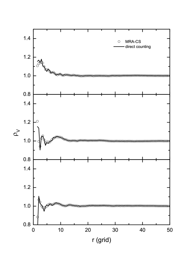
In the first numerical experiment, we randomly placed a sphere center in a poisson sample with $256^{3}$ particles in a $256^{3}$ grid, and then measure the numbers of particles within a sequence of the concentric spherical shells at different radius. Figure 1 plots the volume-average density vs. radius for three randomly placed concentric sphere shells. Clearly, the results calculated from our fast algorithm shows an excellent agreement with the exact values.

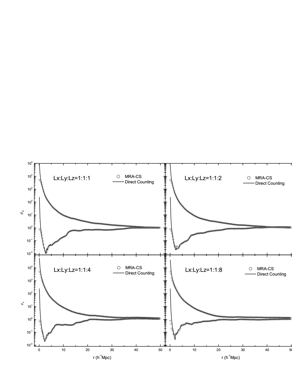
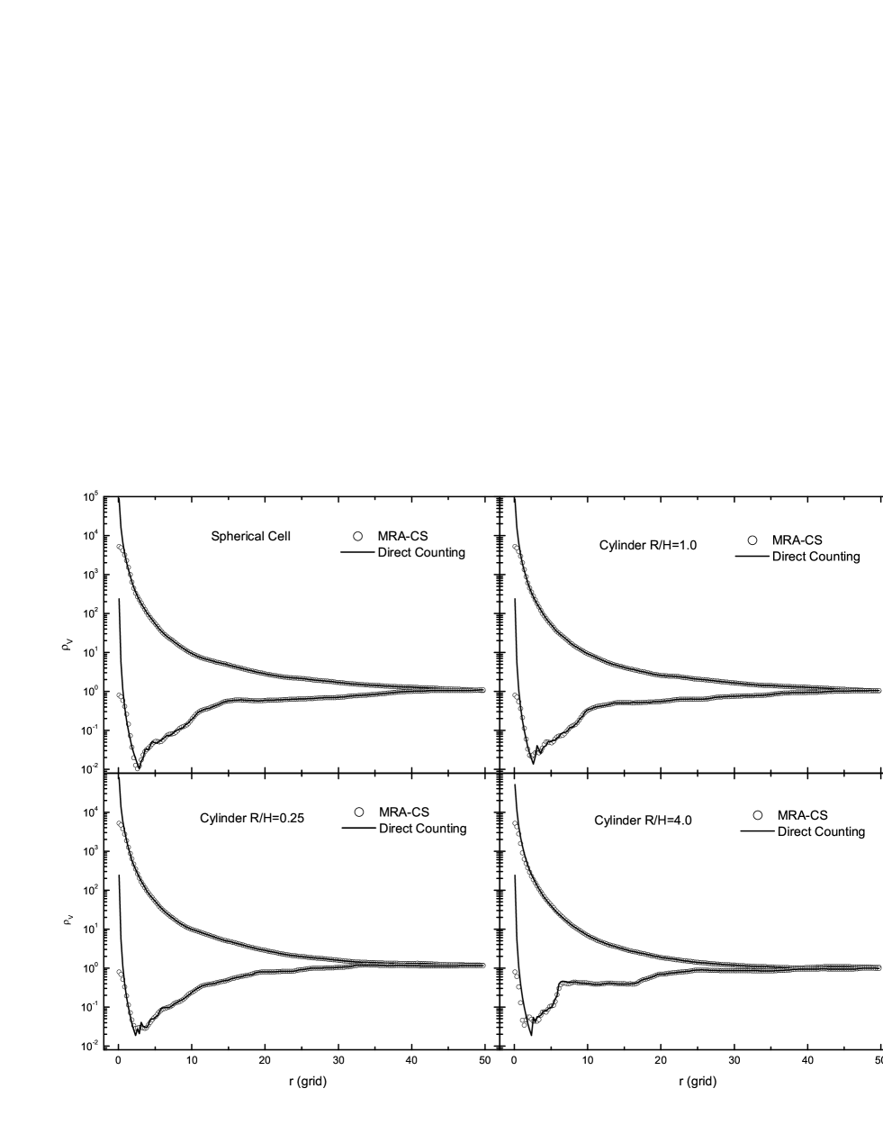
We perform further numerical experiment to test the counts-in-cells with different geometries using the Virgo simulation sample in a $512^{3}$ grid. We have done two sets of the counts-in-cells tests. One was made for fixing the center of cells in a selected particle within a massive halo, and another is for a low density region. The results for the counts in cubic cells are demonstrated in figure 2, where each panel is for cubes with a specific value of the aspect ratio. The horizonal axis is denoted by the equivalent radius of spheres with the same volumes as the cubic cells. Obviously, except for those at scales of a few grids, the MRA-CS algorithm matches with the exact counting very well. Similar results are displayed in figure 3 for the spherical and cylinder counts-in-cells.

It is worthwhile to note that, at small scales, there are visible differences between the MRA-CS and exact counting. Actually, in the MRA-CS scheme, the Fourier transformation of the B-spline of order $n$ is a low pass filter with a sharp suppression $1/k^{n+1}$ of power. Consequently, the Poisson shot noise and fluctuations at short wavelengths will be suppressed. This kind of behavior can be viewed clearly in both figure 2 and figure 3. In case for the counts-in-cells within the massive halo (the upper curve in each panel), as the effect of shot-noise is not significant at small scales, such a suppression leads to the volume-average densities calculated from the MRA-CS scheme being systematically lower than the direct counting as indicated in figure 2. While in the less dense region(the lower curve in each panel), the shot noise dominates at small scales, there are significant fluctuations in the volume-averaged density obtained by direct counting. In comparison, the MRA-CS gives slightly smooth variations of the density with radius.

To have a visual inspection of accuracy of the MRA-CS method, we measure the counts-in-cells using $256^{3}$ spherical cells randomly thrown in the simulation sample, and make a scatter plot in figure 4 to compare the volume-averaged density calculated from the MRA-CS versus those by the direct counting. In order for a good view of errors, the volume-averaged densities are plotted in logarithmic scales. The upper and lower panel display the results for the cell sizes of $R=5$h^-1Mpc and $R=10$h^-1Mpc, respectively. Figure 4 shows more clearly the effects of shot noise occurred in both cases. In the case $R=5$h^-1Mpc, the larger scatters appear in low density regions where sparse sampling makes shot noise more significant than in dense regions. Increasing the size of cell will lead to, on average, more sampling particles in cells, and consequently, the overall scatters tend to be squashed rather smaller. In other words, for a given density, large cells contain more particles than those in small cells, and the effect of Poisson noise in the large cells should be less significant than in the small cells accordingly. This kind of phenomena has been actually illustrated in figure 4 by comparing the case of $R=5$h^-1Mpc (upper panel) with $R=10$h^-1Mpc (lower panel).

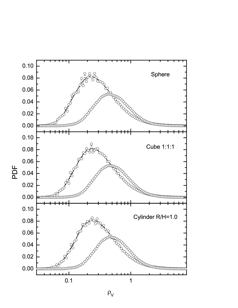
Moreover, in figure 5, we display the probability distribution functions (PDF) of the counts in cells for $R=5$h^-1Mpc and $R=10$h^-1Mpc with three different shapes. In calculations, we used 180 bins to make the PDFs. Basically, there is an excellent agreement of the MRA-CS calculation and the direct counting. In the case $R=5$h^-1Mpc, the PDFs compiled from the direct counting shows slight fluctuations in the low density regions $\rho_{V}<0.5$ due to the effect of shot noise. In comparison, such fluctuations have been smoothed out in the MRA-CS calculations. Whereas in case of $R=10$h^-1Mpc, the direct counting and MRA-CS shows a very good agreement as shown in figure 5. It indicates again that the shot noise could be reduced with increasing cell sizes. This demonstration does show how a reliable statistics could be worked out through the MRA-CS technique.

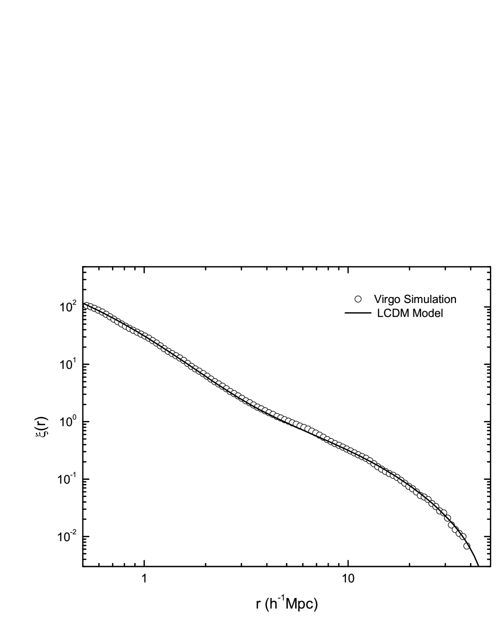
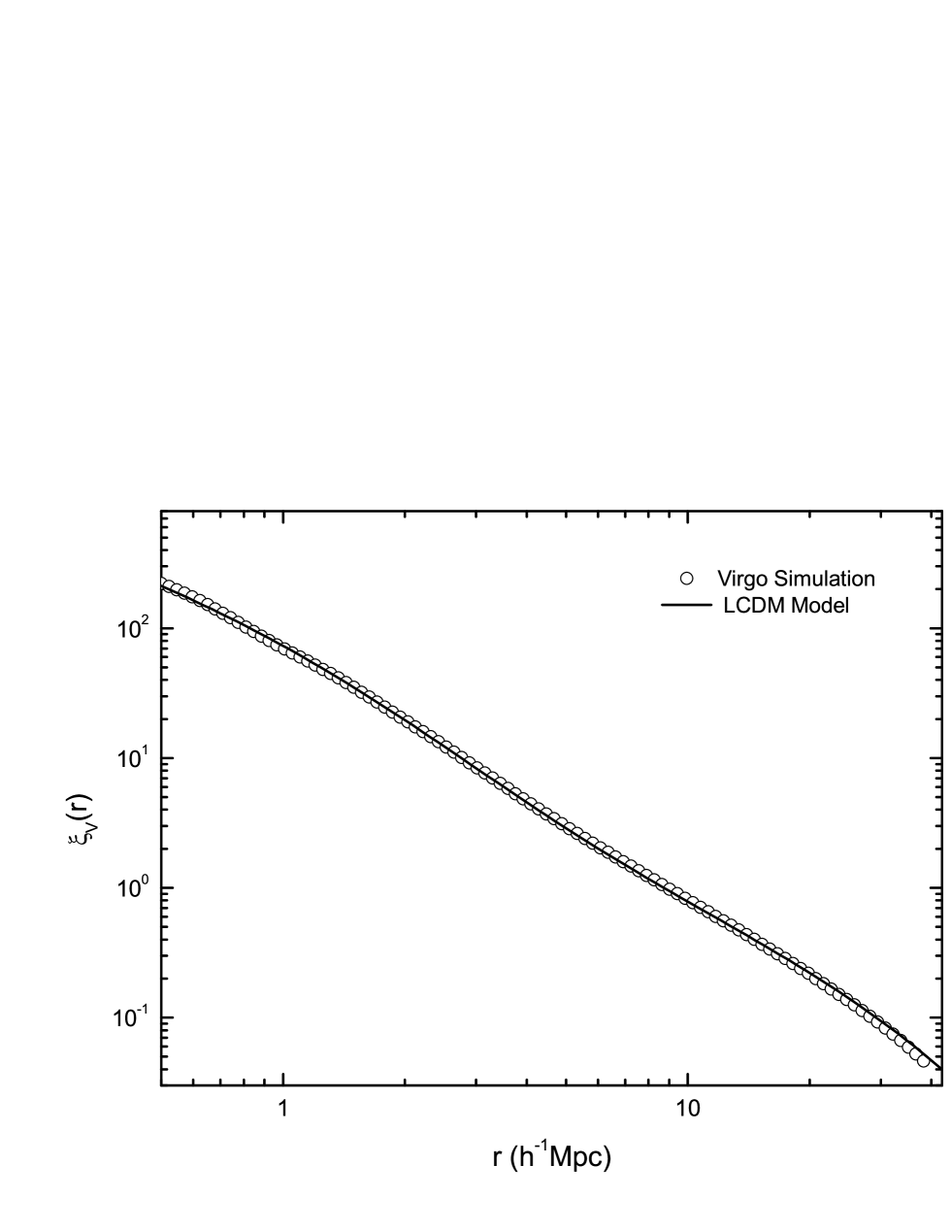
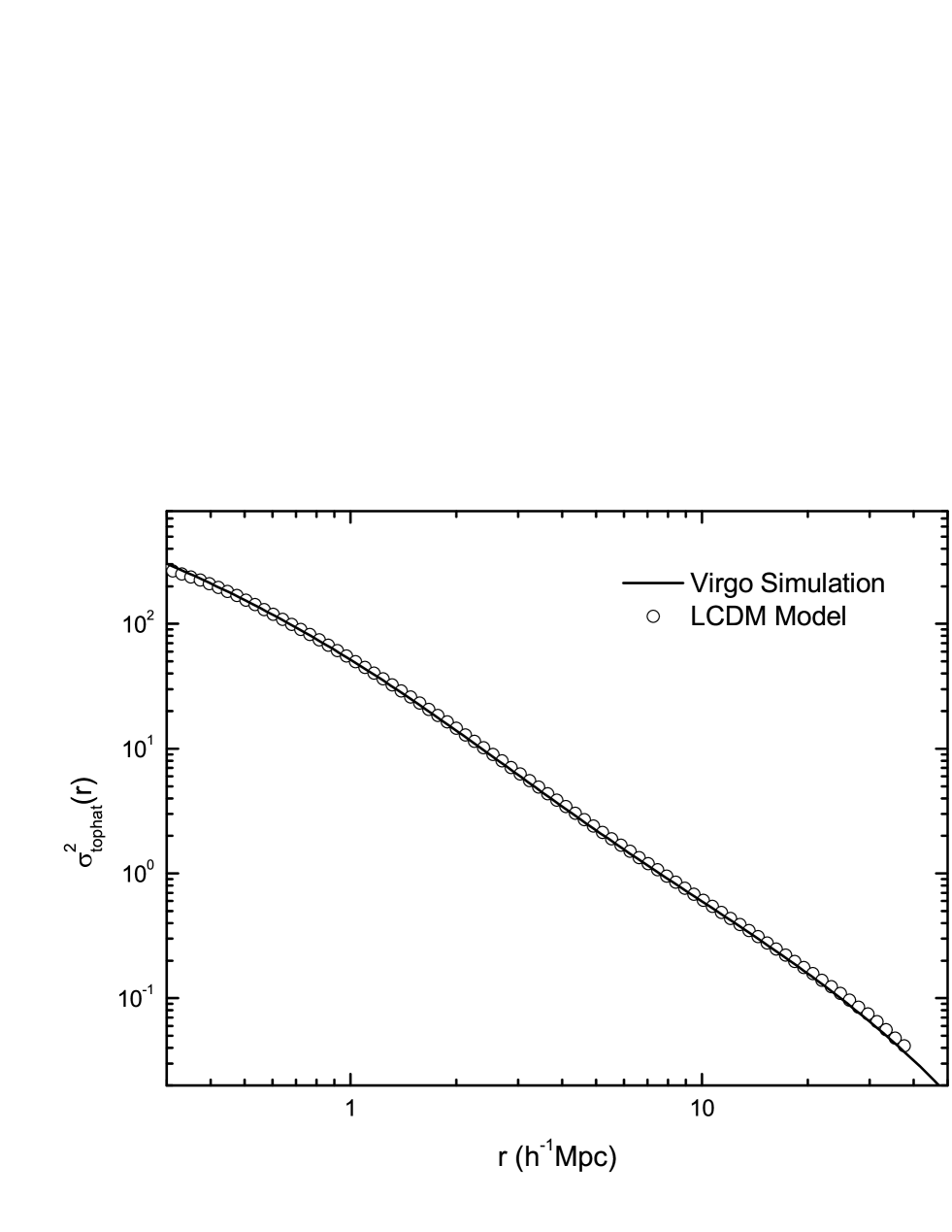
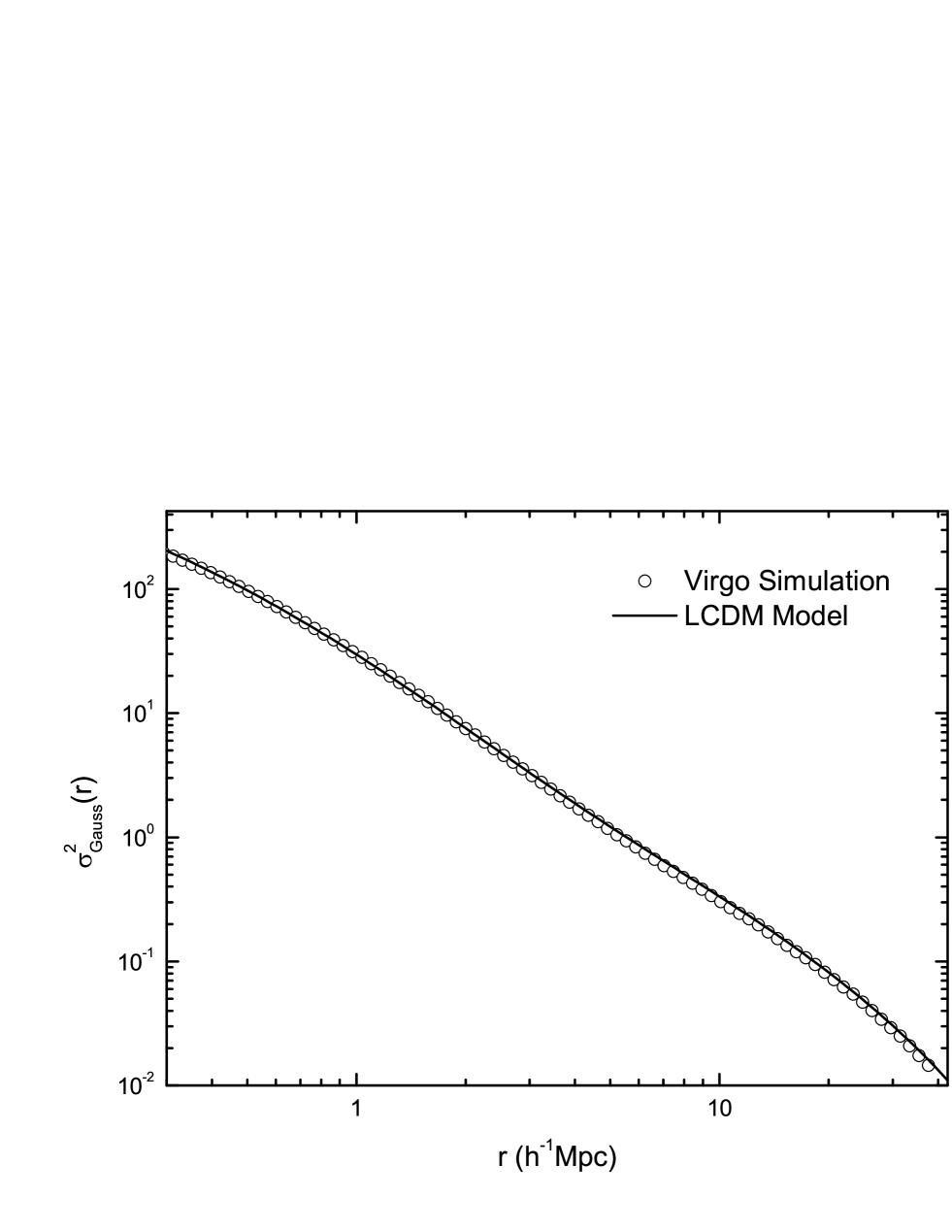
In further applications of the MRA-CS scheme, we measured the second order statistics in the Virgo sample using the fast algorithm described in §2.3. A $512^{3}$ grid has been used, and the physical grid size is thus $0.47$h^-1Mpc. The results include the spatial two-point correlation function in figure 6, the volume-averaged two-point correlation function in figure 7, the variance of density fluctuations by the top-hat filter in figure 8 and the Gaussian filter in figure 9, respectively. In all figures, we also plot the theoretical curves using the fitting formulae of nonlinear power spectrum in LCDM models (Smith et al, 2003). The agreement of our fast algorithm with the theoretical model looks quite perfect in scales down to the grid size.

The current implementation of the MRA-CS algorithm is written in Fortran-90. Compiling on a SGI Altix350 workstation of 16 Intel$\circledR$ Itanium 2 1.5G CPUs with the OPENMP parallelization, it runs at the speed of 1.6 seconds per $256^{3}$ counts-in-cells using B-splines of degree $n=5$. By the scaling, a massive counts-in-cells measurement with $10^{9}$ sampling cells could be done with 2 minutes in the same machine. In the computations, the Intel$\circledR$ Math Kernel Library (MKL) has been also applied to perform the fast Fourier transformations.

Finally, it is necessary to point out that, the central idea in the MRA-CS scheme is to find a finite and smooth representation of discrete particle distribution, which is a singular function as given by the Dirac delta function in eqn.(1). In principle, the higher is order of B-splines, the better is approximation to the Dirac function (see Appendix 3). However, as computational cost is scaled as $(n+1)^{d}$ where $n$ is the order of B-splines and $d$ is the dimension of space, the higher order B-splines may leads to less efficient in the algorithm. To set up a compromise between them, we have numerically tested the dependence of accuracy on orders of B-splines. The result indicates that for $n\geq 5$, there are no visual differences at scales larger than the grid size. Accordingly, we have used the fifth order of B-splines throughout this paper.

4 Discussions and Concluding Remarks

We have described a fast algorithm of cosmic statistics based on multiresolution analysis, in which fields or operators are decomposed in term of a set of orthonormal compactly supported bases at various levels of details. This method naturally leads to a fast summation rule, and could find wide applications in different areas. In application to cosmic statistics, we made an implementation of the MRA-CS scheme using high order B-spline biorthogonal bases and justified its efficiency and reliability by the numerical experiments. Using spherical,cubic and cylinder counts in cells, we found that the MRA technique yields good estimations of the counts-in-cells. On small scales, there appear some discrepancies in comparison with direct counting. In statistics, it is not negative. Actually, weak signals in a point process suffer from the Poisson shot noise. However, in the MRA-CS scheme, those high frequency shot noises could be suppressed by the virtue of the fast decaying behavior of sharp low pass filters.

Based on the MRA-CS scheme, we proposed further a fast algorithm to estimate the two-point spatial correlation function. Strikingly, we proved that, taking average of pair counts over a sample can be simplified to a vector product. That is, the averaged pair counts can be obtained without counting. Is is also shown that this method can be generalized to calculate other second order statistical quantities such as the variances of cosmic fields filtered with arbitrary window functions. Using the simulation sample, we demonstrate an excellent agreement between our MRA-CS method and the theoretical expectation.

The MRA-CS algorithm has several advantages,

(1) It is a grid-based algorithm making use of the FFT technique, and thus is significantly faster than the conventional counts in cells methods.

(2) In particular, the algorithm does not slow down while extending to large scales. Actually, the number of operations required using this method is independent of cell sizes. Therefore, this method enable us to perform a massive sampling to reduce statistical errors.

(3) The algorithm can be, in principle, applied to sampling cells with arbitrary shapes, so as their spatial configurations could be well defined mathematically.

When measuring the counts-in-cells in real galaxy samples, there are two observational effects needed to be taken into account. The first is volume incompleteness due to bright star masks and complicated survey geometry. In the former, holes around bright stars should be excavated, and in the latter some sampling cells beyond boundary contain some fraction of space that are not in the survey volume. The another effect is spectroscopic incompleteness. There are several schemes suggested so far to correct galaxy counts in cells for real samples ( e.g. Efstathiou et al. 1990, Croton et al. 2004). For instance, in the Croton et al.’s approach applying to the 2dFGRS catalogue, they first estimated the combined spectroscopic and volume completeness factor $f$ using the survey mask and then compensate the missed volume by expanding the cell such that the resized incomplete cell has the same volume as the ideal fully complete cell. Subjecting to the numerical tests, this method is likely to give reasonable results.

This paper makes no attempt to discuss the issue of incompleteness in detail. Here, we only brief a simple scheme to tackle this problem. Practically, we may generate a uniform particle distribution with the survey mask applied, and then compute its SFCs. When estimating galaxy count within a cell in the real data using the MRA-CS method, the same measurement is also performed in the marked uniform sample. Actually, measuring the counts-in-cells in the marked uniform sample may yield a good estimation of the completeness factor $f$ so as it is dense enough. Explicitly, the completeness factor $f$ for a cell is equal to its volume-averaged density if the mean density of the unmarked uniform sample is taken to be unity. It is basically an alternative to the current Monto-Carlo method for computing irregular spatial volumes. In the proceeding step, we may fix an acceptable minimum value of the completeness factor $f_{c}$, sampling cells with $f<f_{c}$ are excluded, otherwise, we may apply Croton et al’s volume compensation algorithm for galaxy counts in the re-scaled cells.

Statistically, the more information could be extracted by sampling in larger configuration spaces of counts-in-cells. In fact, the non-Gaussianities characterized by the high order statistics in the cosmic fields are produced by the highly non-linear mode-mode coupling, which may manifest itself in gravitational collapse or merging of dark matter halos. Therefore, examining the shape dependence of high order statistics might be helpful to understand gravitational clustering pattern, e.g., the topology and large scale structure, morphologies of voids, filaments and their networks, and the origin of biasing. It is expected that the MRA-CS technique developed in this paper could provide an efficient tool for investigating the higher order statistical features in the large scale structure of the universe.

The MRA-CS scheme has been implemented in a set of subroutines, which is publicly available upon request to the author.

Appendix A B-splines

A.1 Definition and Basic Properties

B-splines are symmetrical, bell shaped functions constructed from the $n+1$ fold convolution of a rectangular pulse $\beta^{(0)}(x)$:

$$\beta^{(0)}(x)=\left\{\begin{array}[]{r@{\quad\quad}l}1&if|x|<0.5\\ 0.5&if|x|=0.5\\ 0&otherwise\end{array}\right.$$ (A1)

$$\beta^{(n)}(x)=(\beta^{(0)}_{+1}\circ\beta^{(0)}_{+2}\circ\cdot\cdot\cdot\beta^{(0)}_{+n}\circ\beta^{(0)}_{+(n+1)})(x)$$ (A2)

where the symbol $\circ$ denotes for operation of convolution. $\beta^{(n)}(x)$ is a piecewise polynomial of degree n,

$$\beta^{(n)}(x)=\sum_{l=0}^{n+1}(-1)^{l}{n+1\choose l}\frac{(x+\frac{n+1}{2}-l)^{n}_{+}}{n!}$$ (A3)

In practical calculation, the B-splines could be obtained using recursion over the spline order,

$$\beta^{(n)}(x)=\frac{(n+1)/2+x}{n}\beta^{(n-1)}(x+1/2)+\frac{(n+1)/2-x}{n}\beta^{(n-1)}(x-1/2)$$ (A4)

The Fourier transformation of $\beta^{(n)}(x)$ is related to the $n+1$ fold convolution construction of the B-splines,

$$\hat{\beta}^{(n)}(\xi)=\Bigl{(}\frac{\sin\pi\xi}{\pi\xi}\Bigr{)}^{n+1}$$ (A5)

The $n$-th order B-spline has a compact support of $[-\frac{n+1}{2},\frac{n+1}{2}]$. As $\beta$ is not orthogonal to its translates, we apply the orthgonalizatio scheme to construct its dual base $\gamma$, such that

$$\int_{-\infty}^{\infty}\beta^{(n)}(x-k)\gamma^{(n)}(x-l)dx=\delta_{kl}$$ (A6)

It follows from above orthogonality condition that, in the wavenumber space,

$$\hat{\gamma}^{(n)}(\xi)=\frac{\hat{\beta}^{(n)}(\xi)}{a^{(n)}(\xi)}$$ (A7)

with the periodic function

$$a^{(n)}(\xi)=\sum_{l=-\infty}^{\infty}|\hat{\beta}^{(n)}(\xi+l)|^{2}=\sum_{l=-n}^{n}\beta^{(2n+1)}(l)e^{i2\pi l\xi}$$ (A8)

It is noted that the dual scaling function $\gamma$ is not compactly supported.

A.2 Kernel Representation Using B-spline Biorthogonal Bases

For a given kernel $W(x,y)$, it could be decomposed in terms of B-splines $\beta$ (Beylkin & Cramer, 2002),

$$W(x,y)=\sum_{k}\sum_{l}w_{k-l}\beta(x-k)\beta(y-l)$$ (A9)

it follows from the orthogonality eq.(A6) that the coefficients $\{w_{n}\}$ can be found formally by

$$w_{n}=\int\gamma(x-n)(W\circ\gamma)(x)dx$$ (A10)

Since $\gamma$ can be expressed as a linear combination of B-splines, we have

$$\gamma(x)=\sum_{-\infty}^{\infty}q_{k}\beta(x-k)$$ (A11)

Substituting eq.(A11) into eq.(A10), we have

$$w_{n}=\sum_{m}\tilde{q}_{n-m}\zeta_{m}$$ (A12)

in which,

$$\tilde{q}_{m}=\sum_{k}q_{k}q_{m+k}$$ (A13)

and

$$\zeta_{n}=\int\beta(x-n)(W\circ\beta)(x)dx$$ (A14)

Taking Fourier transformation on both sides of eq.(A11), we may see that the coefficients $\{q_{n}\}$ are Fourier coefficients of the function $1/a(\xi)$, and the coefficients $\{\tilde{q}_{n}\}$ in eq.(A13) are Fourier coefficients of the function $1/[a(\xi)]^{2}$. Define the trigonometric series $\hat{w}$ and $\hat{\zeta}$ by

$$\hat{w}(\xi)=\sum_{-\infty}^{\infty}w_{n}e^{i2\pi n\xi}$$ (A15)

and

$$\hat{\zeta}(\xi)=\sum_{-\infty}^{\infty}\zeta_{n}e^{i2\pi n\xi}$$ (A16)

Thus, Fourier transformation of eq.(A12) implies

$$\hat{w}(\xi)=\frac{\hat{\zeta}(\xi)}{[a(\xi)]^{2}}$$ (A17)

Obviously, eqs.(A15)(A16) and (A17) formulate an algorithm of obtaining $w_{n}$ directly from $\zeta_{n}$.

Let the central B-spline $\beta$ is of odd degree $M-1$, then support of $\beta(x)$ is $\{x:|x|\leq M/2\}$. Hence, eq(A14) can be written in form of

$$\zeta_{n}=\int^{M}_{-M}B(x)W(x+n)dx$$ (A18)

where $B(x)=\int\beta(x+y)\beta(y)dy$ is the autocorrelation of $\beta(x)$, which is supported on the interval $\{x:|x|\leq M\}$. If the kernel $W(x,y)$ does not have singularity in whole axis $\bf R$, just as either spherical or cubic kernel considered in this paper, the integral eq.(A10) is convergent, and only finite number of the coefficients $\zeta_{n}$ are nonzero. For the singular operator such as that of the power law $1/x^{\alpha}$, the regularization procedure is necessary, the integral in eq.(A10) may fail to converge for all integer $n$, because $\gamma(x-n)$ fails to vanish in a neighborhood of the singularity of the kernel $W$. The detail for regularization scheme based on the multiresolution approach could be found in Beylkin and Cramer (2002).

A.3 Approximation to the $\delta$-Function

Let $n(x)=\delta(x-x_{0})$ in eq.(17), and the scaling function is taken to be B-splines, $\phi_{j,l}(x)=\beta^{(n)}_{j,l}(x)$, using the dual of $\beta$, then we have the finite representation of $\delta$-function from eq.(18)

$$\delta(x-x_{0})\rightarrow n^{j}_{0}(x)=\sum_{k\in{\bf Z}}\beta^{(n)}_{j,k}(x_{0})\gamma^{(n)}_{j,k}(x)$$ (A19)

It could be proven that, if $w$ is a test function, $w\in C^{\infty}$ , then

$$w(x_{0})=\int_{-\infty}^{\infty}n^{j}_{0}(x)w(x)dx+O(h^{n+1})$$ (A20)

where $h=2^{-j},j>0$ (Beylkin, 1995).

Figure 1: Spherical counts in cells: volume-averaged density varies with radius measured in a sequence of concentric spherical shells placed in a random sample with $256^{3}$ particles. The MRA-CS results(circules) are compared with the direct counting (solid line). The upper, central and lower panels display the results in three numerical experiments respectively

Figure 2: The volume-averaged density measured in the Virgo simulation sample as a function of cell size for a fixed center of cells. Each panel corresponds to a given aspect ratio as indicated in the figure, and plots two sets of the counts in cells measurements. One is made in a massive dark matter halo (upper curves), and another is for a low density region (lower curves). The figure compares the results obtained from the MRA-CS algorithm (open circules) with the direct counting (solid line).

Figure 3: Same as fig.(2), but for spherical and cylinder counts in cells. For the cylinder cells, the aspect ratio is indicated in each panel.

Figure 4: Spherical counts in cells: the volume-averaged density calculated by the MRA-CS scheme versus those from the direct counting. The measurements were made in the Virgo simulation sample. The $3\times 10^{4}$ scatters (circule) randomly chosen from a total $256^{3}$ sampling are displayed. The upper panel is for the cell size $R=5$h^-1Mpc and the lower panel for $R=10$h^-1Mpc.

Figure 5: Comparison of the probability distribution function of volume-averaged density obtained from the MRA-CS algorithm (solid line) with that by direct counting (circule). The counts in cells are performed in the same simulation sample as in fig.2. The upper, middle and lower panels display the results for spherical, cubic and cylinder cells. In each panel, the right and left curves denote results for cells with the equivalent radius $R=5$h^-1Mpc and $R=10$h^-1Mpc respectively.

Figure 6: The two-point correlations function measured with the MRA-CS alogrithm (open circules) in the Virgo LCDM sample vs. the nonlinear power spectrum given by Smith et.al (2003)(solid line). In the MRA-CS calculation, a $512^{3}$ grid has been used.

Figure 7: Same as fig.6, but for the integral two-point correlation function.

Figure 8: Same as fig.6, but for the variance of the top-hat filtered density field.

Figure 9: Same as fig.6, but for the variance of the Gaussian filtered density field.