A New Multidimensional Hydrodynamics code based on Semidiscrete Central and WENO schemes.

Abstract

We present a new multidimensional classical hydrodynamics code based on Semidiscrete Central Godunov-type schemes and high order Weighted Essentially Non-oscillatory (WENO) data reconstruction. This approach is a lot simpler and easier to implement than other Riemann solver based methods. The algorithm incorporates elements of the Piecewise Parabolic Method (PPM) in the reconstruction schemes to ensure robustness and applications of high order reconstruction schemes. A number of one and two dimensional benchmark tests have been carried out to verify the code. The tests show that this new algorithm and code is comparable in accuracy, efficiency and robustness to others.

1 Introduction

Gas dynamics and their simulations are of considerable interest in many areas of astrophysics. Computational astrophysics is now one of the main branches of theoretical astrophysics that provide invaluable tools for studying complex astrophysical phenomena. The areas in which computational tools have proved absolutely necessary in astrophysics have mainly involved fluid/gas flows and N-body simulations. Such flows are described by nonlinear equations that can be expressed as hyperbolic conservation laws and may contain shock waves as solutions. These equations cannot be treated analytically in multi-dimensions and hence one must rely on numerical approximations to study them. Using standard finite difference techniques to handle shock waves, discontinuities etc., usually lead to spurious oscillations and instabilities in the solution that render these approaches useless for tackling most astrophysical scenarios of interest. Therefore non-standard approaches are necessary to deal with these problems. High resolution shock capturing schemes (HRSC) are a class of numerical methods devoted specifically to this purpose. The key feature of such methods is their ability to accurately approximate the solution in smooth regions while also handling shock waves and discontinuities away from them. Due to its wide ranging applications HRSC scheme research is one of the most active areas of research in applied mathematics. For an introduction and a pedagogical review of HRSC schemes we refer the reader to Levequque R. (1998), Toro (1999), Levequque R. (2002) and references therein.

Computational astrophysics has benefited immensely from HRSC research based on which numerous codes have been developed to study astrophysical fluid dynamics. Among the many HRSC schemes that have been developed for applications in astrophysics one of the most significant is the Piecewise Parabolic method (PPM) of Colella $\&$ Woodward (1985-1,2). Several multidimensional, multipurpose codes have been developed based on the PPM technique and it remains the most often-applied HRSC approach in computational astrophysics (for Eulerian grid based schemes). Some of the recent astrophysical legacy codes based on the PPM approach are the ZEUS (Stone & Norman (1992)), the PROMETHEUS (Fryxell et al. (1989)) and more recently the FLASH (Fryxell et al. (2000); Calder et al. (2002)) codes. Some of these codes have been in development for years and are designed to incorporate new features within their structure as progress is made in Applied Mathematics/Numerical analysis. Based on the experience gained from the development of these codes, the computational astrophysics community has learned that the path from the inception of a particular HRSC scheme to its robust application (for multidisciplinary use) usually requires years of development. The issues borne out by multidisciplinary applications are used to fine tune algorithms and make them as robust and user friendly as possible. Therefore most of the legacy codes mentioned above were designed using HRSC schemes whose inception preceded the codes by years and despite the flexibility of incorporating newer techniques, many recent advances in HRSC research have not been incorporated into these codes. For example, research in areas such as Essentially Non Oscillatory data reconstructions (ENO) (Harten et al. (1987)) methods and Central Godunov type schemes (Nessyahu & Tadmore (1990)) have made good progress and are much simpler than conventional shock capturing schemes. But to date they have not seen widespread applications in computational astrophysics. As astrophysical simulations become more complex and computationally demanding, we need to study the suitability of these newer, simpler algorithms in computational astrophysics. With these issues in mind the purpose of this work is to take the first few steps and lay the foundation toward the development of an efficient, robust, multi-purpose astrophysical hydrodynamics code using a new HRSC scheme that is simpler and relatively inexpensive (computationally) but is as accurate as some of the legacy codes.

Before we introduce the algorithm and the code, we begin by reviewing the main areas of research in HRSC schemes that are essential to understanding the code presented here. In principle, HRSC schemes deal with discontinuities by high order numerical approximations away from shock waves and low order approximations around them. Accuracy and stability are the two main issues to consider when developing HRSC algorithms. These issues are addressed by two main areas of research. These are, the HRSC formulations used to advance the solution in space and time and the non-oscillatory data reconstruction technique, which ensures that the algorithm avoids spurious oscillations when interpolating the data. Each of these are introduced in turn.

First, the formulation of HRSC schemes is considered. In general, two main approaches have been used for formulating HRSC schemes. These are the $Upwind$ (Harten A. (1983); Van Leer B. (1979)) and the $Central$ $Godunov$ type schemes (Lax P. (1954); Friedrichs K. (1954)). Their main difference is that in the central approach the solution is advanced on a staggered grid. This difference has far reaching consequences with respect to the simplicity, efficiency and accuracy of the respective methods. Most hydrodynamic codes, and in particular the multi-purpose legacy codes mentioned above in computational astrophysics are almost exclusively based on the upwind approach. The main reason for this is that upwind schemes are generally less dissipative than central schemes. And until recently, progress has been slow in developing high order, less dissipative central schemes.

Although robust, upwind methods are generally computationally expensive and complicated to implement. This is because upwind methods require computations of the eigenvalues and eigenvectors of the Jacobian of the flux matrix as well as flux splitting and other complicated computations for advancing the solution. In contrast, the central approach is much simpler. Unlike their upwind counterparts, they are computationally less expensive and do not require the computations of eigenvectors, eigenvalues, flux splitting etc. Mainly because of this, much effort has been made recently on the development of central schemes that are as accurate as their upwind counterparts. Some recent advances in central-type HRSC schemes include their high order extensions, semidiscrete, genuinely multidimensional formulations, unstructured grid formulations etc. Among these, the most significant are the semidiscrete formulations (Kurganov & Tadmore (2000)) of central schemes which are much less dissipative than all other previous central approaches. Despite this progress, surprisingly few computations have been done using the central approach in computational astrophysics. In fact, no detailed study has been done to test their suitability for astrophysical simulations besides some very recent ones that are mentioned below and which were done concurrently with this work.

The other main aspect of HRSC research is the development of non-oscillatory data reconstruction techniques. Data reconstruction is an integral aspect of any HRSC scheme and it involves the interpolation of a given set of data that may contain discontinuities over the computational domain. Two of the main techniques for non-oscillatory data reconstructions include the PPM method of Colella & Woodward (1985-2) and ENO approach of Van Leer B. (1979); Osher & Tadmor (1988); Harten A. (1983); Harten et al. (1987). Recently, a newer approach known as the Weighted Essentially Non-Oscillatory (WENO) (Liu L. et al. (1994)) reconstructions scheme, that can be considered an extension of the ENO approach, have also been developed. Each of these reconstruction methods have their own advantages and disadvantages and they have all been shown to perform well for both upwind and central schemes. Even though the PPM method has been used extensively in many legacy codes, the relatively newer WENO schemes have had a comparatively smaller number of applications despite the fact that they are generally more accurate than other reconstructions schemes. Also, they admit arbitrarily high order formulations which can be useful for computations requiring high level of accuracy.

Rapid developments in central schemes research and WENO data reconstruction methods are duly attracting the attention of the computational astrophysics community. Based on progress made in the areas mentioned above, both semidiscrete central and WENO schemes are beginning to be applied. Among these applications the following are noteworthy; Balsara D. (2001), has used the WENO and the upwind approach extensively for multidimensional Magnetohydrodynamics simulations. Recently Feng $\&$ Shu (2004), have applied the WENO technique for cosmological simulations. Del Zanna $\&$ Bucciantini (2002), and Anninos $\&$ Fragile (2003), have developed central-type relativistic hydrodynamic codes and applied it to the study of pulsar bow shock structures (Del Zanna & Bucciantini (2004)) and accretion disks close to black holes (Anninos & Fragile (2004)), respectively. Lucas-Serano et al. (2004), have investigated the suitability of using the semidiscrete central schemes in relativistic hydrodynamics. For multidisciplinary applications, extensions of the central schemes of Kurganov $\&$ Tadmore (2000), is also being considered for integration into the FLASH (Fryxell et al. (2000); Calder et al. (2002)) code. One interesting aspect about all these works is that none of them combine the central approach with the WENO data reconstruction technique that admits high order formulations. For this reason, we have considered a different formulation of the central approach for solving the multidimensional Euler equations and coupled it with a reconstruction scheme that is a combination of the WENO and the PPM reconstruction techniques. Specifically, we consider the central semidiscrete formulation of Kurganov $\&$ Levy (2000), (KL) in which the central semidiscrete scheme is coupled to a 3^rd order WENO reconstruction scheme for solving hyperbolic conservation laws. KL have demonstrated the compatibility of combining the semidiscrete central scheme with a 3^rd order WENO reconstruction algorithm for solving general hyperbolic equations. This was a step forward in HRSC research as it opened the possibility of combining arbitrarily high order accurate WENO reconstruction schemes within the semidiscrete central paradigm. Following them, we propose here a new algorithm for data reconstruction that can be used with the central scheme of KL for robust applications in computational astrophysics. Essentially, the simplicity of central schemes, the accuracy of WENO reconstruction method and the robustness of the PPM algorithm have been combined in this new algorithm. This algorithm has been tested by an extensive collection of one and two dimensional problems with the Euler equations using both 3^rd and 4^th order reconstructions. Many of the tests presented here are a first using the semidiscrete central WENO approach. In particular, the two dimensional Riemann Problems presented in this work are the first such set of computations using the WENO reconstruction scheme. In addition to testing the code, these computations address some other issues with respect to the robust application of WENO schemes for shock capturing schemes that will be discussed later. Building on the work presented here, we have also developed a multidimensional relativistic hydrodynamics code that will be presented in a forthcoming paper.

The outline of this paper is as follows. Sec. 2 presents a brief review of the semidiscrete central scheme and the WENO data reconstruction methods. The hydrodynamics algorithm is then presented in Sec. 3. Sec. 4 presents the tests of the algorithm for the Euler equations. Sec. 4.1 presents the one dimensional test and Sec. 4.2 presents the two dimensional tests. Some concluding remarks are in Sec. 5.

2 Semidiscrete Central and WENO schemes: A Review

This section begins with a brief overview of Godunov type central schemes and the motivations behind their semidiscrete formulation. WENO data reconstruction schemes are also discussed and some of their advantages over other non-oscillatory reconstruction schemes are highlighted. This is followed by a step by step account of the particular central scheme used in our algorithm. This follows a description of the WENO reconstruction scheme used in the code.

The first central scheme was developed by Lax (1954), followed by Frieidrichs $\&$ Lax (1971) (LxF). These schemes were both first order schemes. They were extended to second order by Nessyahu $\&$ Tadmore (1990) (NT). Since then, there has been a number of formulations of the central approach which can be considered extensions of the LxF and NT schemes. These newer formulations explored a number of numerical approaches and applications that improved upon their predecessors. These include high order extensions in multidimensions (Liu & Tadmore (1980); Jiang & Tadmore (1998); Levy et al. (2000, 2002); Kurganov & Petrova (2001); Kurganov & Noelle (2001); Kurganov & Levy (2000)), genuinely multidimensional formulation (that include fluxes from diagonal directions in multidimensions) (Kurganov & Petrova (2001); Kurganov & Noelle (2001)) and recently, the formulation of central schemes on unstructured grids (Kurganov A., Petrova G. (2005)). As mentioned above, the main advantage of central schemes over their upwind counterparts is their simplicity. These schemes do not require the use of computationally expensive Riemann solvers to advance the solution. However, the trade-off for their simplicity is accuracy. In general, central schemes are more dissipative than upwind schemes. To address this issue, Kurganov $\&$ Tadmore (2000) (KT), developed a newer formulation of central schemes known as the semidiscrete central schemes. Numerical tests by KT showed that for central schemes of a given order, semidiscrete central ones were far less dissipative than their predecessors. Hence, these schemes retained the advantages of the central formulation while enhancing its performance. Semidiscrete schemes are different from their predecessors mainly in two ways. First, the solution is advanced on a non-staggered grid. This means that after advancing the solution, it need not be projected back to the original grid. Second, semidiscrete schemes are more accurate because local speed of propagation of information are taken into account in their formulation. The success of the KT scheme precipitated a flurry of research in semidiscrete schemes which included their extensions to higher orders and their multidimensional formulations (Kurganov & Petrova (2001); Kurganov & Noelle (2001); Kurganov & Levy (2000)) among others that will be mentioned later.

We turn now to the WENO data reconstruction methods. WENO schemes were first proposed by Liu et al. (1994), as a natural extension to ENO schemes. The main advantage of WENO over ENO schemes is their arbitrary high order formulations. They are also more accurate then their ENO counterparts. An interesting feature of WENO schemes is that they show “super convergent” behavior not observed in other non-oscillatory data reconstruction methods. Because of these, WENO schemes were incorporated with central schemes by Levy et al. (Levy et al. (1999, 2000, 2002, 2000)) who proposed a new class of HRSC schemes called the Central Weighted Essentially Non-Oscillatory (CWENO) method. In order to take advantage of the characteristics of semidiscrete schemes mentioned earlier and WENO reconstruction methods, Kurganov $\&$ Levy (2000) (KL) combined the semidiscrete central and WENO methods and proposed a new HRSC scheme. This work proved the compatibility of WENO within the central framework. The work presented here is based on the scheme by KL. In some respects, it can even be considered as an extension of the scheme by KL.

The next section (Sec. 2.1) provides a step by step description of the development of central Godunov type schemes and presents the scheme by KL that is used in this work. For the sake of simplicity, a one dimensional scalar hyperbolic conservation law will be considered. The extension to multidimensions and that of a system of equations can be done using standard techniques such as dimensional splitting (Toro (1999)) and other methods. The description of KL will be followed by that of the 3^rd and 4^th order WENO reconstruction scheme used in this work (Sec. 2.2).

2.1 Semidiscrete Central Scheme

Consider the following equation along with the given initial condition

$$u_{t}+\frac{\partial f(u)}{\partial x}=0\quad$$

$$u(x,t=t^{n})=u^{n}(x)\quad.$$ (1)

Our objective is to numerically advance the solution of this equation from $t=t^{n}$ to $t=t^{n+1}$. In order to discretize the problem the following notations are defined. Let $x_{j}:=j\Delta x$, $x_{j\pm\frac{1}{2}}:=(j\pm\frac{1}{2})\Delta x$ and $t^{n}:=n\Delta t$, where $\Delta x$ and $\Delta t$ are unit intervals in space and time respectively. Also define the interval $I_{j}:=[x_{j-1/2},x_{j+1/2}]$ and $u_{j}^{n}$ $:=$ $\{u(x,t=t^{n});$ $x\in I_{j}\}$. The problem may now be summarized as follows; given $u(x,t=t^{n})=\{u_{j}^{n}\}$, we would like to find $\{u_{j}^{n+1}\}$. Alternatively, for finite volume methods that HRSC schemes are, cell averages instead of point values are updated. Defining

$$\overline{u}(x):=\frac{1}{\Delta x}\int_{I(x)}u(\zeta,t)d\zeta\quad,$$ (2)

$$I(x)=\Big{\{}\zeta:|\zeta-x|<\frac{\Delta x}{2}\Big{\}}\quad,$$

and integrating in space, Eq. 1 becomes

$$\overline{u}_{t}(x,t)=\frac{1}{\Delta x}\Big{\{}f(u(x+\frac{\Delta x}{2},t))-f(u(x-\frac{\Delta x}{2},t))\Big{\}}\quad.$$ (3)

Now integrating in time from $t=t^{n}$ to $t=t^{n+1}$ gives,

$$\overline{u}(x,t+\Delta t)-\overline{u}(x,t)=\frac{1}{\Delta x}\left[\int_{t^{n}}^{t^{n+1}}f(u(x+\frac{\Delta x}{2},\tau))d\tau-\int_{t^{n}}^{t^{n+1}}f(u(x-\frac{\Delta x}{2},\tau))d\tau\right]\quad.$$ (4)

This equivalent formulation is the starting point for the construction of Godunov-type schemes for numerically approximating hyperbolic conservation laws. In Eq. 4, the solution is evolved in terms of sliding averages. Setting $x=x_{j}$ leads to a formulation that is known as the upwind scheme. The upwind scheme requires the evaluation of the flux integrals on cell boundaries, where the data could be discontinuous. This is customarily done by using Riemann solvers. On the other hand setting $x=x_{j+1/2}$ leads to the central scheme formulation. Under this scheme, the flux integrals are evaluated at the center of the cell where the data is continuous and finite speed of propagation of information guarantees that Riemann solvers are not needed. Approximations of Godunov type central schemes generally involve three main steps; reconstruction, evolution and projection. The next few paragraphs describe these steps.

First consider the reconstruction step. In this step, given $\{\overline{u}_{j}^{n}\}$, an $nth.$ order, non-oscillatory piecewise polynomial interpolation $\{p_{j}^{n}(x)\}$ of the data is constructed over the computational domain. The $\{p_{j}(x)\}$’s are polynomials that can only be discontinuous at cell interfaces (if the data contains discontinuities) and they are determined from two main constraints. These are, the conservation of cell averages

$$\int_{x_{j-1/2}}^{x_{j+1/2}}p_{j}^{n}(\zeta)\quad{\rm d}\zeta=\overline{u}_{j}^{n} \quad\forall\quad j\quad,$$ (5)

and accuracy requirements

$$u(x,t^{n})=\sum_{j}p_{j}^{n}(x,t^{n})\chi_{j}(x)+O(\Delta x^{r})\quad,$$ (6)

where $\chi_{j}$ is the characteristic function of each cell defined as

$$\chi_{j}(x)=\begin{array}[]{cc}1&{\rm if}\qquad x\in\quad I_{j}\\ 0&\quad{\rm otherwise}\quad.\end{array}$$

The simplest interpolation is of course the piecewise constant case, i.e., $p_{j}^{n}(x,t^{n})=\overline{u}_{j}^{n}$, which leads to the central LxF scheme. Higher order polynomials lead to better approximations but more oscillations near discontinuities. The general strategy used to manage these oscillations is to lower the order of the interpolation near discontinuities. This is known as non-oscillatory reconstruction and ENO and WENO schemes mentioned above are examples of such interpolation.

Once the data reconstruction is done the RHS of Eq. 4 can be computed to advance the solution in time. Using this reconstruction, we may write $u(x,t^{n})\approx\sum_{j}p_{j}^{n}(x)\chi_{j}$. Substituting this in Eq. 4 and setting $x=x_{j+1/2}$ leads to the the following reformulation of Eq. 4

$$\overline{u}_{j+\frac{1}{2}}^{n+1}=\frac{1}{\Delta x}\left[\int_{x_{j}}^{x_{j+\frac{1}{2}}}p_{j}^{n}(x)dx+\int_{x_{j+\frac{1}{2}}}^{x_{j+1}}p_{j+1}^{n}(x)dx\right]-$$

$$\frac{\lambda}{\Delta t}\left[\int_{t^{n}}^{t^{n+1}}f(u(x_{j+1},t))dt-\int_{t^{n}}^{t^{n+1}}f(u(x_{j},t))dt\right]\quad,$$ (9)

where $\lambda=\frac{\Delta t}{\Delta x}$. The first two integrals in in Eq. 7 can be computed exactly given an appropriate piece-wise polynomial interpolation. The flux terms can be approximated by quadrature rules of the appropriate order. The function values needed in the quadrature formula can be computed by using Taylor expansion or the appropriate Runge-Kutta method. For example, using the second order reconstruction of Nessyahu and Tadmore (1990) (NT),

$$p_{j}^{n}(x)=\overline{u}_{j}^{n}+s_{j}^{n}(x-x_{j})\quad,$$ (10)

and using the midpoint rule for flux evaluation results in the NT staggered scheme,

$$\overline{u}_{j+\frac{1}{2}}^{n+1}=\frac{1}{2}(\overline{u}_{j}^{n}+\overline{u}_{j+1}^{n})-\frac{1}{8}(\overline{s}_{j}^{n}-\overline{s}_{j+1}^{n})-$$

$$\lambda\left[f(\overline{u}_{j+1}^{n+1/2})-f(\overline{u}_{j}^{n+1/2})\right]\quad,$$ (11)

where $s_{j}^{n}$ is constructed using $minmod$ limiters to minimize oscillations. For example,

$$s_{j}^{n}={\rm minmod}(\frac{\overline{u}_{j}^{n}-\overline{u}_{j-1}^{n}}{\Delta x},\frac{\overline{u}_{j+1}^{n}-\overline{u}_{j}^{n}}{\Delta x})\quad,$$ (12)

where the $minmod$ function is defined as,

$${\rm minmod}(a,b):=\frac{{\rm sgn(a)}+{\rm sgn(b)}}{2}{\rm min}(|a|,|b|)\quad.$$ (13)

Eq. 9 is the second order NT scheme and Eqns. 8, 10 are an example of a second order ENO data reconstruction method. All modern central schemes can be thought of as extensions of the scheme by NT including the KL scheme presented below. As mentioned earlier, numerical experiments with the NT scheme show this approach to be numerically dissipative and in order to address this issue, Kurganov $\&$ Tadmore (2000) (KT) derived the semidiscrete version of the central scheme. The derivation of this approach is complicated and for details we refer the reader to Kurganov & Tadmore (2000). The semidiscrete scheme that we have used is a further extension of the KT scheme and uses a 3^rd order WENO data reconstruction method. It was presented in KL and is given by

$$\frac{d}{dt}\overline{u}_{j}(t)=-\frac{H_{i+\frac{1}{2}}(t)-H_{i+\frac{1}{2}}(t)}{\Delta x}\quad,$$ (14)

where the flux $H_{i+\frac{1}{2}}$ is given by

$$H_{i+\frac{1}{2}}(t):=\frac{f(u^{+}_{i+\frac{1}{2}}(t))+f(u^{-}_{i+\frac{1}{2}}(t))}{2}-$$

$$\frac{a_{i+\frac{1}{2}}(t)}{2}\left[u^{+}_{i+\frac{1}{2}}-u^{-}_{i+\frac{1}{2}}\right].$$ (15)

where $u^{+}_{i+\frac{1}{2}}$, $a_{i+\frac{1}{2}}$ are given by,

$$a_{i+\frac{1}{2}}:=\max\{\rho(\frac{\partial f}{\partial u}(u_{j+1/2}^{-})),\rho(\frac{\partial f}{\partial u}(u_{j+1/2}^{+}))\}$$ (16)

$$u^{+}_{i+\frac{1}{2}}=P(x_{j+1/2})\quad.$$ (17)

In Eqns. 13 and 14, $a_{i+\frac{1}{2}}$ is the speed of propagation of $u$ at the interface of a cell that is determined from the spectral radius of the Jacobian of the flux $f$. Using Eq. 12, the solution can be updated by any high order Total Variation Diminishing (TVD) Runge-Kutta type ODE solver.

The extension of the scheme presented above to multi-dimensions can be done as follows. Eq. 12 in multidimensions contains flux contributions from every dimension that can be determined as in the one dimensional case. This leads to an unsplit scheme, which is what is used in our algorithm.

2.2 WENO Reconstruction Scheme

Since its inception, WENO (Liu L. et al. (1994)) data reconstruction schemes have been improved and incorporated into a number of HRSC schemes and have also been applied to a number of problems in computational astrophysics. WENO schemes posses most of the advantages of the ENO methods and some significant others that ENO schemes do not have. The main advantage is their arbitrarily high order formulations. In this work we have implemented a 3^rd and a 4^th order WENO reconstruction schemes given by Kurganov & Levy (2000) and Levy et al. (2002, 1999), respectively. The following reproduces the details of the 4^th order scheme presented in Levy et al. (1999). Whenever necessary, the modifications needed for the 3^rd order reconstruction scheme have also been highlighted. For simplicity, only the one dimensional reconstruction scheme is described here. Multidimensional extensions of the scheme presented here can be done using dimensional splitting in a straight forward manner.

Our task is as follows; given $\{\overline{u}_{j}^{n}\}$, we would like to construct a 4^th order piecewise parabolic interpolation of the data $u^{n}(x)$ over the computational domain. Described below is the reconstruction procedure for a single interval $I_{j}$. The same procedure can be extended to interpolate the data over the entire domain. The main idea of the WENO approach is as follows. Let $R_{j}(x)$ be the non-oscillatory interpolant over the cell $I_{j}$. It is given by a weighted convex combination of interpolation polynomials $p_{k}(x)$ (where k = j, j+1, j-1), constructed over different stencils. This weighted combination is used to ensure that the interpolant receives the most significant contribution from the smoothest stencil, thereby preserving the non-oscillatory character of the interpolation. Therefore, $R_{j}(x)$ is given by

$$R_{j}(x)=w_{j-1}^{j}p_{j-1}^{j}(x)+w_{j+1}^{j}p_{j+1}^{j}(x)+w_{j}^{j}p_{j}(x)\quad.$$ (18)

The $w_{k}^{j}$’s are weights corresponding to each polynomial and are subject to the normalization constraint

$$\sum w_{k}^{j}=1\quad.$$ (19)

The computations of the weights will be described shortly. The polynomials $p_{k}(x)$’s are constructed by using different stencils around the point $x_{k}$ where k = $\{j,j+1,j-1\}$. For example, $p_{j-1}(x)$ is the polynomial based on the left stencil $\{x_{j-3},x_{j-2},x_{j-1},x_{j},x_{j+1}\}$. Other polynomials are constructed similarly. The coefficients of the polynomials $p_{k}(x)$ are fixed by satisfying the following conservation and accuracy requirements,

$$\frac{1}{h}\int p_{j}(x)dx=\overline{u}_{k},\qquad k=j-1,j,j+1,$$ (20)

$$\frac{1}{2h}\int p_{j}(x,t^{n})\quad dx=\frac{1}{2h}\int u(x,t^{n})\quad dx+O(h^{s})\quad.$$ (21)

Therefore writing the polynomials as,

$$p_{j}(x)=\tilde{u}_{k}+\tilde{u}_{k}^{\prime}(x-x_{k})+$$

$$\frac{1}{2}\tilde{u}_{k}^{\prime\prime}(x-x_{k})^{2},\qquad k=j-1,j,j+1$$ (22)

and applying conditions set by Eqns. 18 and 19 gives,

$$\tilde{u}_{k}^{\prime\prime}=\frac{\overline{u}_{k+1}-2\overline{u}_{k}+\overline{u}_{k-1}}{h^{2}}\quad,$$ (23)

$$\tilde{u}_{k}^{\prime}=\frac{\overline{u}_{k+1}-\overline{u}_{k-1}}{2h}\quad,$$ (24)

$$\tilde{u}_{k}=\overline{u}_{k}-\frac{h^{2}}{24}\tilde{u}_{k}^{\prime\prime}\quad.$$ (25)

Note: In case of 3^rd order reconstruction Kurganov & Levy (2000), the polynomials $p_{j-1}^{j}(x)$ and $p_{j+1}^{j}(x)$ are piecewise linear. The method for computing their coefficients is the same as that shown above.

The weights $w_{k}^{j}$ $(k=j-1,j,j+1)$ are given by (for details, see Jiang G-S, Shu C-W (1996)),

$$w_{k}^{j}=\frac{\alpha_{k}^{j}}{\alpha_{j-1}^{j}+\alpha_{j}^{j}+\alpha_{j+1}^{j}}\quad,$$ (26)

where

$$\alpha_{k}^{j}=\frac{C_{k}}{(\epsilon+IS_{k}^{j})^{p}},\quad C_{k}>0\quad.$$ (27)

The constants $C_{k}$ are known as $optimal$ $weights$ and their evaluation is described in Shu & Osher (1988). The parameter $IS_{k}^{j}$ is used to compute the smoothness of the various stencils and is defined below. The parameter $\epsilon$ is needed to prevent the denominator of $\alpha_{k}^{j}$’s from going to zero. From Eqns. 24, 25 above we note that the parameters $C_{k}$, $p$ and $\epsilon$ are the only free parameters in WENO reconstruction schemes. They must be set a priori depending on the application being considered. However numerical tests have shown that some specific choice seems to work well for a number of test problems. For example when computing point values, any symmetric combination of $C_{k}$ gives the desired order of accuracy. The parameter $p$ is empirically chosen and is set to 2 for 3^rd order schemes and 3 for 4^th order schemes. The parameter $\epsilon$ is usually set to $10^{-6}$. For our computations we have kept the values corresponding to the 3^rd and 4^th order schemes fixed. This was done deliberately to test the robustness of our algorithm.

The smoothness indicators $IS_{k}^{j}$ are defined by,

$$IS_{k}^{j}=\sum_{l}\int h^{2l-1}(p_{k}^{l})^{2}\quad dx,\quad k=j-1,j,j+1\quad.$$ (28)

These represent the $L^{2}$ norms of the first and second derivatives, where $p_{k}^{(l)}$ denotes the $l^{th.}$ derivative of $p_{k}^{j}(x)$. For our 4^th order reconstruction, the smoothness indicators are given by

$$IS_{j-1}^{j}=\frac{13}{12}(\overline{u}_{j-2}-2\overline{u}_{j-1}+\overline{u}_{j})^{2}+\frac{1}{4}(\overline{u}_{j-2}-4\overline{u}_{j-1}+3\overline{u}_{j})^{2}\quad,$$

$$IS_{j}^{j}=\frac{13}{12}(\overline{u}_{j-1}-2\overline{u}_{j}+\overline{u}_{j+1})^{2}+\frac{1}{4}(\overline{u}_{j-1}-\overline{u}_{j+1})^{2}\quad,$$

$$IS_{j+1}^{j}=\frac{13}{12}(\overline{u}_{j}-2\overline{u}_{j+1}+\overline{u}_{j+2})^{2}+$$

$$\frac{1}{4}(3\overline{u}_{j}-4\overline{u}_{j+1}+\overline{u}_{j+1})^{2}\quad.$$ (29)

For a system of equations, some modifications are necessary for computing the smoothness indicators $IS_{k}$. Even though computations can be done component wise, best results are obtained by using universal smoothness indicators Kurganov & Levy (2000). They are given by,

$$IS_{k}=\frac{1}{d}\sum_{r=1}^{d}\frac{1}{\parallel\overline{u}_{r}\parallel_{2}}(\sum_{l=1}^{2}\int_{x_{j-1/2}}^{x_{j+1/2}}h^{2l-1}(p_{k,r}^{l})^{2}\quad dx)\quad,$$

$$k\in{j-1,j,j+1}\quad.$$ (30)

Where $d$ is the number of equations. The scaling factor $\parallel\overline{u}_{r}\parallel_{2}$ is defined as the $L^{2}$ norm of the cell averages of the $r^{th}$ component of $u$ defined by,

$$\parallel\overline{u}_{r}\parallel_{2}=(\sum_{j}|{\overline{u}}_{j,r}|^{2}h)^{1/2}.$$ (31)

This completes the description of the 4^th. order WENO reconstruction scheme. We now present some tests of the scheme used in our hydrodynamics code. Consider the function $f(x)$ $=\sin(x)$, where $x\in[0,2\pi]$. Tables 1 and 2 below shows the $L^{1}$ and $L^{\infty}$ errors for reconstructing $f(x)$ using the schemes described above. The free parameters of WENO reconstructions ($C_{i}$’s, $\epsilon$ and $p$) are the same as those from Kurganov & Levy (2000), Levy et al. (1999). There are several interesting features worth noting from these results. For the 4^th order reconstruction (Table 2), the order remains constant around four as the mesh spacing is decreased, as is expected. However for the 3^rd order scheme (Table 1), non-linear behavior can be noticed in the errors. In fact, the reconstruction becomes better than order three and shows the so called “super convergent” behavior noted by Liu L. et al. (1994) when they introduced WENO reconstructions. This non-linear super convergence will also be seen in some of the tests of our hydrodynamic codes.

3 The Multidimensional Hydrodynamics Algorithm

In principle, the combination of the WENO reconstruction scheme with the central semidiscrete scheme is adequate for solving general hyperbolic conservations laws. However, if one demands a robust scheme for general applications, then the scheme above would require modifications as the standard WENO prescriptions given above is still too oscillatory for cases in which shock waves are very strong. How the WENO schemes could itself be modified to handle such strong shocks is an interesting research project in numerical analysis. However, given our objective of building a robust hydrodynamic code, this is beyond the scope of this work. Instead, to ensure robustness for our applications, we have considered certain elements of the PPM scheme and incorporated these into our data reconstructions scheme. The features of the PPM scheme that makes the algorithm presented here robust are its contact steepening, flattening and monotonicity preserving algorithms. These steps are outlined in detail in Colella $\&$ Woodward (1985-2). We have incorporated them into our algorithm without any modification. We discovered that when semidiscrete central WENO schemes are combined with these extra, it is robust with respect to a large number of benchmark tests (see Sec. 4). Our hydrodynamic algorithm can be summarized as follows,

step 1: Given ${\overline{u}}_{j}^{n}$, use the $nth.$ order WENO reconstruction algorithm to construct ${p_{j}(x,t^{n})}$. Use the $p_{j}(x,t^{n})$’s to compute $u_{j}^{+}$, $u_{j}^{-}$ .

step 2: Apply the steepening (only to the density $\rho$), flattening and monotonicity preserving algorithms to $u_{j}^{+}$, $u_{j}^{-}$ (Eq. 15) .

step 3: Update ${\overline{u}}_{j}^{n}$ to ${\overline{u}}_{j}^{n+1}$ using the scheme described in Sec 3.1 (Eq. 12).

In step 3 of the algorithm above, we have used a total Variation diminishing (TVD) multi-step Runge-Kutta (RK) ODE solver roe that we give below.

$$U^{(1)}=U^{n}+\Delta TL(U^{n})$$

$$U^{(2)}=\frac{3}{4}U^{n}+\frac{1}{4}U^{(1)}+\frac{3}{4}\Delta tL(U^{(1)})$$

$$U^{n+1}=\frac{1}{3}U^{n}+\frac{2}{3}U^{(2)}+\frac{2}{3}\Delta tL(U^{(2)}).$$ (32)

All our tests have done using this RK scheme.

4 Tests of the Hydrodynamics Code

The standard approach to testing any HRSC scheme consists of simple advection tests; shock capturing using Berger’s equation followed by more complex tests. For the semidiscrete CWENO scheme used here, advection and Berger’s equation related tests have already been published Kurganov & Levy (2000), and while our codes were being developed, we have also reproduced them (without the PPM type modifications mentioned in the last section). However, we do not present the results here. Since our primary interest is in gas dynamics, we present test results of our hydrodynamic code.

In two dimensions, the Euler equations of hydrodynamics are given by

$$\frac{\partial}{\partial t}\left(\begin{array}[]{ll}\rho\\ \rho u\\ \rho v\\ E\end{array}\right)+\frac{\partial}{\partial x}\left(\begin{array}[]{ll}\rho u\\ \rho u^{2}+p\\ \rho uv\\ u(E+p)\end{array}\right)+\frac{\partial}{\partial y}\left(\begin{array}[]{ll}\rho v\\ \rho uv\\ \rho v^{2}+p\\ v(E+p)\end{array}\right)=0\quad.$$

The equations above are closed by an equation of state. For ideal gases this is given by $p=(\gamma-1)(E-\rho/2(u^{2}+v^{2}))$. Here $\rho$, $u$, $v$, $p$ and $E$ are the density, the $x$ and $y$ velocities, the pressure and the total energy respectively. For most of our tests, we have used an ideal gas equation of state for which the adiabatic index, $\gamma$ $=$ $5/3$. The tests chosen for the code follow from those chosen to test the ZEUS and FLASH codes (Stone & Norman (1992); Fryxell et al. (2000); Calder et al. (2002)). In one dimension, these include several advection tests and some standard shock tube problems. In 2D, they include an exhaustive list of Riemann problems and several blast wave tests.

4.1 One Dimensional Tests

As already mentioned, following Stone $\&$ Norman (1992), Fryxell et al. (2000) and Calder et al. (2002), several advection tests were carried out followed by some standard shock tube tests. The results are discussed below and compared to previously published results.

4.1.1 Advection Tests

Advection problems were used to check the ability of our scheme to transport and maintain the shape of a density pulse. The tests presented here were first suggested by Boris & Book (1973); Foreste (1977) and considered by both Stone & Norman (1992) and Fryxell et al. (2000). First, we considered the simple advection of a rectangular and a Gaussian pulse. For example, advecting a rectangular pulse tests the codes ability to lead and trail contact discontinuities while advecting a Gaussian pulse tests its ability to handle narrow flow features. The pulse profile we use for these two test profiles is given by

$$\rho(s)=\rho_{1}\phi(s/w)+\rho_{0}(1-\phi(s/w))\quad,$$ (33)

where $s$ is the distance from of a point from the pulse midplane and $W$ is the characteristic width of the pulse. For the square and Gaussian pulse, the $\phi(x)$ as,

$$\phi(x)=\left\{\begin{array}[]{ll}1&\textrm{if $\mid x\mid<1$}\\ 0&\textrm{if $\mid x\mid>1$}\\ \exp(-x^{2})&\textrm{if pulse is Gaussian}\\ \end{array}\right\}\quad.$$

With this definition, the Euler equation reduces to a simple advection equation.

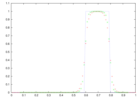
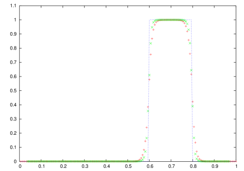
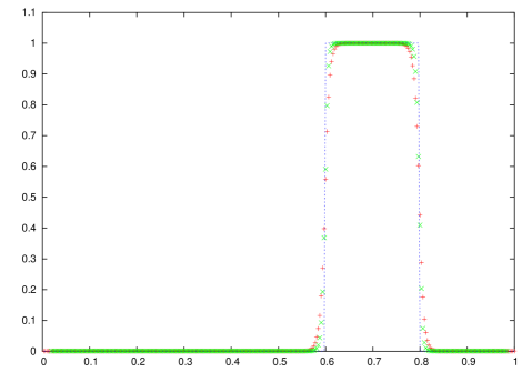
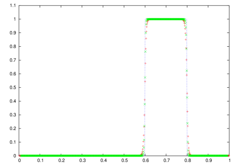
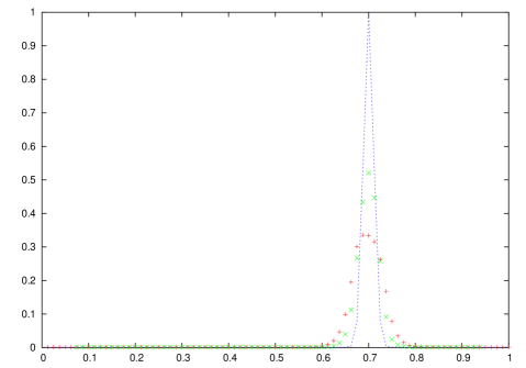
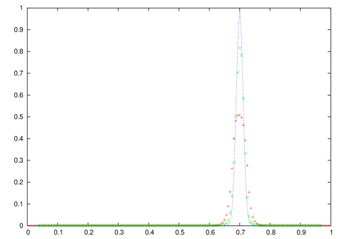
We begin with the rectangular profile. The advection of the rectangular pulse were followed to time $t=0.2$ and the positions of both the advected and the analytic solutions are shown in Figs. 1 and 2 for n=80, 160, 320 and 640. The solution has been plotted using both the 3^rd. and 4^th. order reconstruction schemes and the analytic solutions. Several features can be noted from these plots. First, there is the convergence of the solution with increasing resolution. Second, that the 4^th order reconstruction gives better results than the 3^rd order scheme for the same grid spacings. Finally, comparing our results to those of Stone & Norman (1992), Fryxell et al. (2000), there is good qualitative agreement.

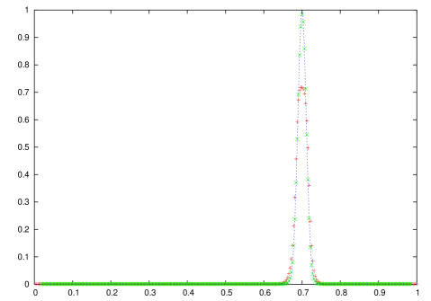
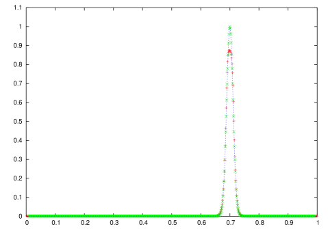
Continuing with the advection of a Gaussian pulse, we set the width of the pulse to $w=.015625$ and advected the pulse to time $t=0.2$. The results are shown in Figs. 3 and 4. Once again, as with the case of the rectangular pulse, there is convergence to the analytical solution as $n$ increases. As expected, the 4^th. order scheme converges faster than the 3^rd. order scheme. We have tabulated the $L1$-error norms of the solution in Table 3 for the 3^rd. and 4^th. order reconstructions. The results show some interesting behavior similar to tests done on this problem by both Fryxell et al. (2000) and Stone & Norman (1992). In general we would expect the schemes to be of high order accuracy away from shocks and discontinuities and of first order accuracy close to discontinuities. When a narrow Gaussian profile is discretized it behaves as neither a discontinuity nor a smooth function. Hence with decreasing mesh spacing the order of convergence is fractional and increasing before it starts to decrease for the 4th order reconstruction.

The next consideration was the propagation of a sinusoidal sound wave consisting of a density and a pressure wave perturbation propagating at the speed of sound, $C_{s}$. The initial conditions are given in Eq. 32 and periodic boundary conditions were applied while propagating the perturbation.

$$\rho=\rho_{0}+\epsilon\rho_{0}\cos(kx)\quad,$$

$$p=p_{0}+C_{s}^{2}(\rho-\rho_{0})\quad,$$

$$v=C_{s}\frac{\rho-\rho_{0}}{\rho_{0}}\quad.$$ (34)

The background density $\rho_{0}=3.0$ and pressure $p_{0}=50.0$, $\epsilon$ is set to $10^{-6}$ and $k$ is the wave number. Shown in Table 4, are the $L_{1}$ norms of density error of our solutions for the 3^rd. and 4^th. order reconstructions.

4.1.2 Shock Tube Tests

Shock tube tests are used to test a codes ability to capture shock waves. In one dimension, shock tube tests can be described as follows. A one dimensional domain of length $l$ is divided into two halves and its initial thermodynamic states specified. The thermodynamic state of the tube is then advanced in time. The initial configurations usually give rise to shock waves, contact discontinuities and rare faction waves whose amplitudes and position can be determined analytically. Any reliable HRSC scheme would be able to capture these shock waves. A collection of standard shock tube tests have been designed to verify various qualities of any given scheme. We begin here by presenting some of these results in one dimension. The flattening and monotonicity preserving sub-steps involve setting some free parameters Colella & Woodward (1985-2). For each test done here, we have indicated the values of these parameters in Table 5 Outflow boundary conditions were used for all our tests unless otherwise specified.

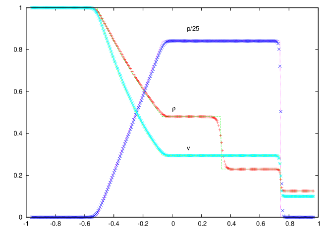
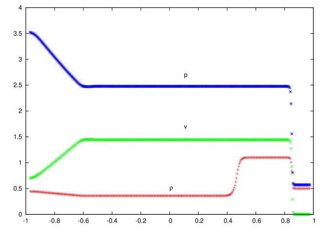
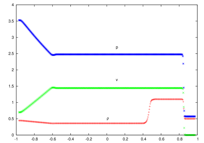
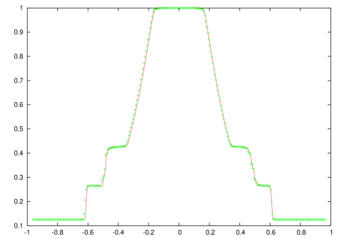
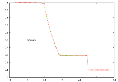
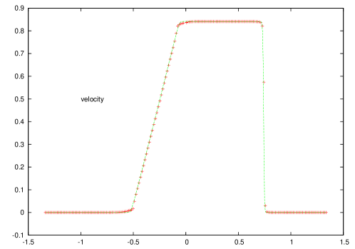
Test 1: We begin with the Sod shock tube test. The initial condition for this test is given by; $\rho_{left}=1.0$, $v_{left}=0$, $P_{left}=1.0$, $\rho_{right}=.125$, $v_{left}=0$, $P_{right}=0.1$. With this initial condition, the following happens. The left pressure being greater than the right one results in a shock wave that will propagate rightward. In addition, the central contact discontinuity that is visible in the density plot propagates rightward, while a rarefaction wave propagates left from its the origin. The results are shown in Fig. 5 where both the numerical and analytical solutions are presented for the 3^rd and 4^th order reconstructions. We note excellent agreement between the analytic and numerical approximations. To complement these results, we have also shown the $L1$ error versus grid spacing of our solutions for both the 3^rd and 4^th order reconstructions in Table 6. The results satisfy the expected first order convergence rate for both reconstructions. Finally, comparing the results to Stone & Norman (1992), Fryxell et al. (2000) and the analytic solution, we note excellent agreement.

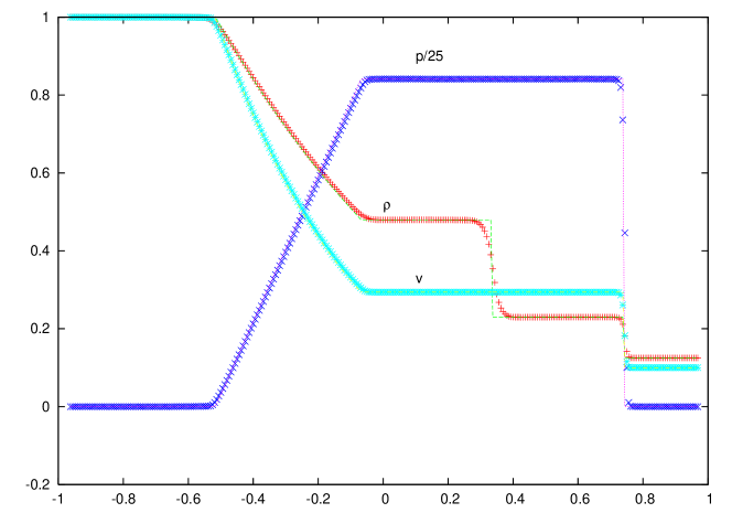
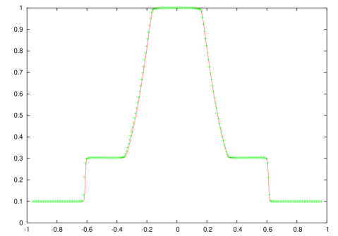
Test 2: The next test is Lax’s Problem (Lax P. (1954)). The thermodynamics state is given by, $\rho_{left}=0.445$, $u_{left}=0.698$, $P_{left}=3.528$, $\rho_{right}=0.5$, $u_{right}=0$, and $P_{right}=0.571$. The density, velocity and pressure profiles are shown in Fig. 6 for both the 3^rd. and 4^th. order reconstructions. Note that the 4^th. order results are marginally better than the 3^rd. order scheme around the shock and contact discontinuities. These results also show good qualitative agreements with those given by Suresh & Huynh (1997).

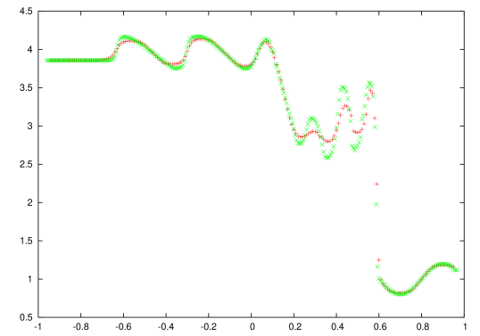
Test 3: The next test is Shu’s Problem (Shu (1990)). This problem is designed to test the ability of the scheme to resolve both a discontinuity as well as an oscillatory solution. The initial state is, $\rho_{left}=3.857143$, $u_{left}=2.629369$, $P_{left}=10.3333$, $\rho_{right}=1.0+0.2\sin(5\pi x)$, $u_{right}=0.0$, $P_{right}=1.0$. The left and right sides are defined as left$:$ $-1<$ x $<-0.8$ and right$:$ $-0.8<$ x $<1.0$. Our results are shown in Fig. 7. There is a noticeable difference between the 3^rd. and 4^th. order reconstructions in this case. We find the 4^th. order solution to be more oscillatory than that using the 3^rd. order results. Qualitatively our results match those obtained by Suresh & Huynh (1997).

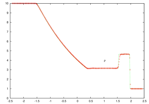
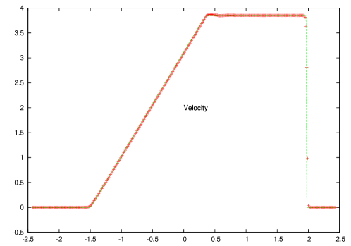
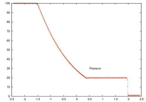
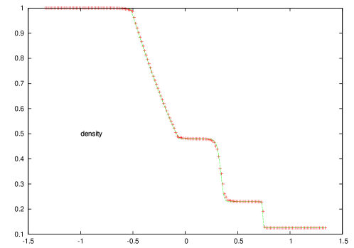
Test 4: The next test is Sod Strong Shock Problem (Fryxell et al. (2000)). This test is designed to capture stronger shocks than any of the above, and hence, is quite challenging. The initial state is, $\rho_{left}=10.0$, $P_{left}=100.0$, $\rho_{right}=1.0$ and $P_{right}=1.0$. The results are shown in Fig. 8. There is excellent agreements between our results and the analytic solution. Also, a direct comparison between our scheme and that of Fryxell et al. (2000) shows good qualitative agreement.

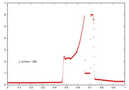
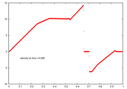
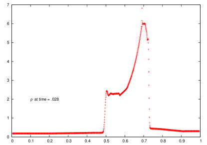
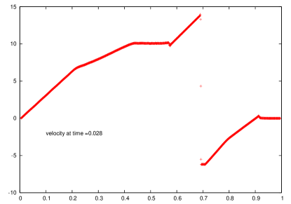
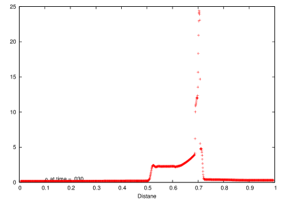
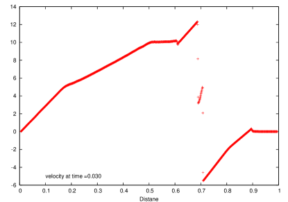
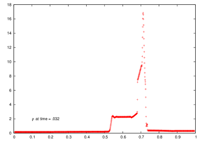
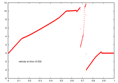
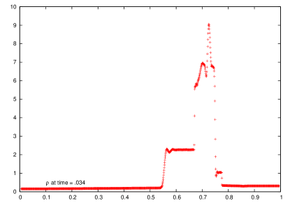
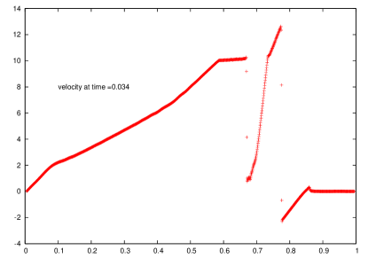
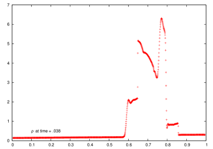
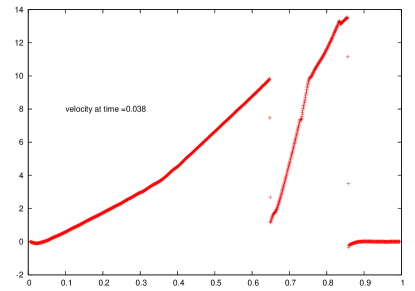
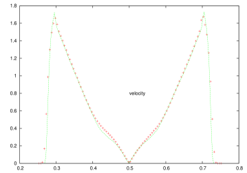
Test 5: The next test is the interaction between two blast waves described by Colella & Woodward (1985-1). The initial state consists of three constant states on the domain $x$ $\in$ $[0,1]$; $\rho_{[0,.1]}=1.0$, $u_{[0,.1]}=1.0$, $P_{[0,.1]}=1000.0$, $\rho_{[.1,.9]}=1.0$, $u_{[.1,9]}=0.0$, $P_{[.1,9]}=.01$, $\rho_{[.9,1.0]}=1.0$, $u_{[0.9,1.0]}=0.0$ and $P_{[0.9,1.0]}=100.0$. Solid reflective boundary conditions are used on the computational domain. This is one of the most demanding tests for an HRSC code. The expected solution structure is as follows; shocks are driven into the middle part of the grid while rarefaction waves propagate toward the outer boundaries. By the time the shocks collide, the rarefaction waves have caught up to them, making their post shock structure complex. For more details of the complexities involved with this test, see Fryxell et al. (2000). Our results are shown in Figs. 9, 10 and 11. The density and velocity profiles are shown from $t=0.026$ (before the shock waves begin to interact) to $t=0.038$ (after they have stopped interacting). These results are compared directly to those of Fryxell et al. (2000) and Stone & Norman (1992) and show excellent qualitative agreement with them.

4.2 2D Riemann Problems using WENO

As was the case in one dimension, the most elementary two dimensional tests of HRSC schemes are 2D shock tube (2D Riemann problem) tests. It can be described as follows. A square computational domain is divided into four quadrants and thermodynamics states specified. The initial data are constant in each quadrant and restricted so that only one elementary wave, a one dimensional shock, a one dimensional rarefaction wave or a two dimensional contact discontinuity appears at each interface. According to Lax $\&$ Liu (1998), the total number of genuinely different configurations for polytropic gases in 2D shock tube tests is nineteen. Lax $\&$ Liu (1998) solved for all nineteen configurations to demonstrate the utility of their so-called $positive$ $Scheme$ (an HRSC scheme). Kurganov $\&$ Tadmore (2002) perform exactly the same calculations to test their HRSC scheme, that was based on ENO reconstructions and a genuinely multidimensional CENO approach. Following these two works, we have performed similar computations to test our scheme. Kurganov $\&$ Tadmore (2002) have demonstrated that the central scheme in combination with an ENO reconstruction scheme does indeed satisfactorily solve the 2D Riemann problems of Lax $\&$ Liu (1998). However, they comment that because WENO reconstruction is based on smoothness indicators, a priori information of the solution structure is necessary for solving the variety of 2D Riemann problems they considered. We demonstrate here that a fixed set of parameters for computing the smoothness indicators solves the 2D Riemann problems without a priori knowledge of the solution structure. To do this, we turned off the steepening, flattening and monotonicity preserving component of our algorithm for these tests. This also allows us to make a direct qualitative comparison between our results and those of Lax $\&$ Liu (1998) and Kurganov $\&$ Tadmore (2002). Hence we have tackled two issues; the WENO related issue just mentioned above as well as testing our algorithm. To describe the initial conditions for our 2D Riemann problems and the initial patterns expected from them, we define the following notations;

$R^{\rightarrow}_{lr}:$ Forward rarefaction wave
$R^{\leftarrow}_{lr}:$ Backward rarefaction wave
$S^{\rightarrow}_{lr}:$ Forward shock wave
$S^{\leftarrow}_{lr}:$ Backward shock wave
$J^{-}_{lr}:$ Positive Slip line
$J^{+}_{lr}:$ Negative Slip line.

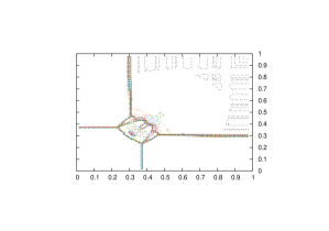
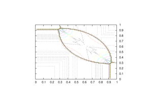
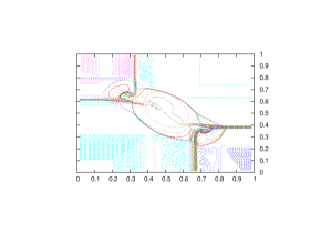
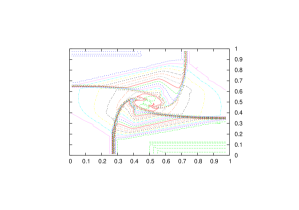
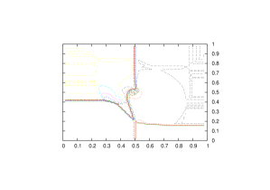
Table 7 gives the wave patterns expected for each of the nineteen configurations. In it, the subscripts represent the wave pattern expected between the quadrants, e.g., $J_{21}^{+}$ means that between the second and the first quadrant, a negative slip line will results from the initial conditions at these two quadrants. The convention used to label the quadrants are as follows. Considering a square, the North-East quadrant is labelled 1, North-East quadrant is labelled 2, South-West quadrant is labelled 3, South-East quadrant is labelled 4. Tables 8-9 presents the initial conditions that give rise to the various wave patterns which are shown in table 7. For details of the thermodynamics conditions that give rise to the various wave patterns, see Lax $\&$ Liu (1998). Each of our computations were done using $n=400$ and the adiabaticity constant $\gamma$ $=$ $1.4$. The time to integration is case dependent. An unsplit algorithm is used to advance the solution in time. We also used the 4^th order, dimensionally split WENO reconstruction in all our calculations in this and the next section. We expect to obtain comparable results with 3^rd order reconstructions.

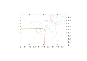
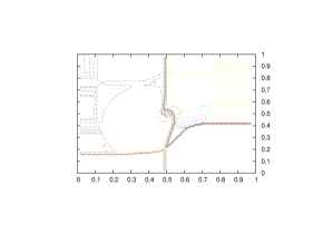
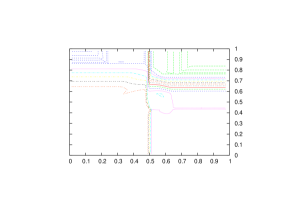
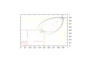
Our results are shown in Figs. 12-16. By direct qualitative comparison with Lax $\&$ Liu (1998) and Kurganov $\&$ Tadmore (2002), it is noted that all features of every configurations obtained by the previous studies have been recovered.

4.3 Some more 2D test Problems

Next we present some other standard tests for multidimensional HRSC schemes. Following Fryxell et al. (2000), and Stone $\&$ Norman (1992), we consider an explosion problem, a two dimensional Sod Shock problem and a Sedov blast wave problem. The purpose of these tests is to verify the robustness of the algorithm for stronger shock waves than the previous tests.

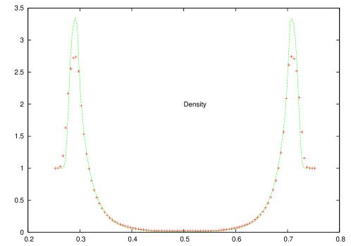
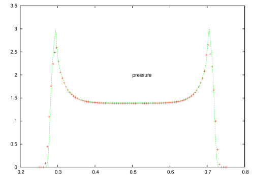
Test 1: The 2D explosion problem. The following initial condition sets off a spherically symmetric explosion; $(\rho,u,v,P)$ $=$ $(1.0,0.0,0.0,1.0)$ if $x^{2}+y^{2}<.2^{2}$, else $(\rho,u,v,P)$ $=$ $(.125,0.0,0.0,0.1)$. The computational domain is a square of length 2 units and the initial high density and pressure region is cantered around the origin. We have shown the density and pressure profiles at time t$=$.25 for n=200 in Fig. 17. The profile shown is along the x-axis of the explosion. The solid line represents the profile obtained from a one dimensional analytical computation. Note that our 2D explosion results are in good agreement with the one dimensional calculations.

Test 2: The 2D Sod shock problem. The thermodynamic state is the same as the 1D Sod shock problem except the membrane separating the two regions is chosen to be along the diagonal of the square region. Shown in Fig. 18 are the density, velocity and pressure profiles along the diagonal of the domain. Similar to the one dimensional test, there is good agreement between the analytical and numerical approximations.

Test 3: The Sedov Blast wave problem. This problem is the self-similar evolution of a cylindrical blast wave from a delta-function initial pressure perturbation in an otherwise homogeneous medium. The initial conditions are exactly those considered by Calder et al. (2002) in their test. We consider a small region of radius $\delta r$ at the canter of the grid. The pressure inside this region is given by

$$p_{0}=\frac{3(\gamma-1)\epsilon}{3\pi\delta r^{2}}\quad.$$ (35)

The ambient pressure is set to $10^{-5}$ and the density is set to $\rho$ $=$ $1.0$ throughout the domain. The gas is assumed to be stationary at time t=0 and we have taken $\delta r$ $=$ $3.5*meshspacing$. For analytical solutions to the problem we refer to Calder et al. (2002). In Fig. 19, we have shown the density, pressure and velocity profiles at time $t$ $=$ $.05$ units. In the same plot we have indicated the analytical solutions as well. We note good agreement between the analytical and computed results.

5 Conclusions and future work

We have tested a new dimensionally unsplit multidimensional hydrodynamics code using a robust, multidimensional HRSC scheme based on central semidiscrete Godunov type schemes, WENO data reconstruction algorithms and the PPM method. To our knowledge, this is the first multi-purpose hydrodynamics code based on this approach that has been developed for computational astrophysics. To ensure robustness, we have modified the standard WENO schemes and added elements of the PPM reconstruction scheme. Our new algorithm and code is tested by a collection of standard one and two dimensional tests. Whenever possible, the results have been compared to the literature and analytic solutions. Overall, both our one and two dimensional codes perform well without having to fine tune some of the user supplied input parameters for a wide range of tests. From the results we may conclude that the algorithm proposed here performs comparably to other HRSC schemes. This success in implementing WENO based codes efficiently takes us a step closer towards using arbitrarily high order data reconstruction schemes in computational astrophysics.

In this context, the present work should be considered as taking the first few steps toward the development of a robust, multipurpose, multidimensional HRSC scheme for computational astrophysics. The reliability and applicability of a given algorithm is best tested by applying it to a variety of problems. This usually exposes potential weaknesses of the algorithm that can then be rectified. It is our intention to apply this code to a number of astrophysical problems. At present, we are considering a multidimensional study of pulsar bow shock structure simulations. We are also planning to study gravitational waveforms emitted by collapsing stars. To extend the code’s capabilities, several extensions are planned for the future. Key among them are an extension to three dimensions, addition of adaptive capabilities and application of the algorithm to Magnetohydrodynamics. In addition, we are also planning to implement the algorithm using MPI for parallel architectures. As mentioned before, there have been a number of other advances of the central semidiscrete schemes that is worth investigating along the lines of this algorithm. These include the genuinely multidimensional formulation of the scheme and the scheme on an unstructured grid, etc. It is clear that there is room for a good deal of work using such algorithms. We look forward to making progress in the future.

N	$L^{1}$-error	Rate	$L^{\infty}$-error	Rate
40	0.00189	-	0.001020	-
80	0.0002815	2.76	0.000254	2.00
160	3.73E-05	2.90	6.17E-05	2.00
320	2.93E-06	3.7	6.92E-06	3.2
640	9.87E-08	4.9	1.49E-07	5.53
1280	2.71E-09	5.2	2.38E-09	6.0

Table 1: $L^{1}$ and $L^{\infty}$ errors for 3^rd. order reconstruction (Sec. 3.2)

N	$L^{1}$-error	Rate	$L^{\infty}$-error	Rate
40	2.64E-05	-	7.80E-06	-
80	1.83E-06	3.86	4.79E-07	4.06
160	1.17E-07	3.96	2.98E-08	4.0
320	7.41E-09	4.03	1.86E-09	4.03
640	4.64E-10	4.00	1.16E-10	4.00
1280	2.90E-11	4.00	7.41E-12	4.00

Table 2: $L^{1}$ and $L^{\infty}$ errors for 4^th order reconstruction (Sec. 3.2)

N	$L^{1}$-error (3rd. order)	Rate	$L^{1}$-error (4th. order)	Rate
40	3.87E-2	-	3.38E-2	-
80	2.67E-2	.53	1.61E-2	1.07
160	1.63E-2	.74	5.19E-3	1.63
320	7.12E-3	1.19	5.04E-4	3.37
640	2.09E-3	1.77	4.27E-05	3.57
1280	5.92E-4	1.82	9.29E-06	2.20
2560	1.38E-4	2.11	1.83E-06	2.35

Table 3: $L^{1}$ errors for the advection of a narrow Gaussian pulse by 3^rd. and 4^th. order WENO reconstruction.

N	$L^{1}$-error (3rd. order)	Rate	$L^{1}$-error (4th. order)	Rate
40	6.59E-07	-	7.56E-08	-
80	8.22E-08	3.01	9.07E-09	3.06
160	1.02E-08	2.93	1.19E-09	2.94
320	1.28E-09	3.00	1.76E-10	2.76

Table 4: $L^{1}$ errors for the advection of a sinusoidal perturbation by 3^rd. and 4^th. order WENO reconstruction.

Test	$K_{0}$	$\eta^{(1)}$	$\eta^{(2)}$	$\epsilon^{(1)}$	$\omega^{(1)}$	$\omega^{(2)}$	$\epsilon^{(2)}$
Test 1	0.10	20.0	0.05	0.1	0.52	10.0	0.1
Test 2	0.10	20.0	0.05	0.1	0.52	10.0	0.1
Test 3	0.10	20.0	0.05	0.1	0.52	10.0	0.1
Test 4	0.10	20.0	0.05	0.01	0.52	10.0	0.33
Test 5	0.10	20.0	0.05	0.01	0.52	10.0	0.33

Table 5: Values of the monotonicity, flattening and contact steepening parameters used for one dimensional shock tube tests presented in Sec. 5.1

N	$L^{1}$-error (3rd. order)	Rate	$L^{1}$-error (4th. order)	Rate
40	4.82E-1	-	1.75E-1	-
80	2.45E-1	0.97	9.99E-02	0.82
160	1.20E-01	1.03	5.01E-02	0.99
320	6.18E-02	0.97	2.47E-02	1.02
640	3.18E-02	0.97	1.25E-02	0.99

Table 6: $L^{1}$-errors in density for the Sod shock tube test for 3^rd. and 4^th. order WENO reconstructions.

Test	$K_{0}$	$\eta^{(1)}$	$\eta^{(2)}$	$\epsilon^{(1)}$	$\omega^{(1)}$	$\omega^{(2)}$	$\epsilon^{(2)}$
Test 1	.10	20.0	0.05	0.1	0.52	10.0	0.33
Test 2	.10	20.0	0.05	0.1	0.52	10.0	0.33
Test 3	.10	20.0	0.05	0.01	0.52	10.0	0.33

Table 7: Values of the monotonicity, flattening and contact steepening parameters used for 2D tests from Sec. 5.3

Configuration	$C_{12}$	$C_{32}$	$C_{34}$	$C_{41}$
Config. 1	$R_{21}^{\rightarrow}$	$R_{32}^{\rightarrow}$	$R_{34}^{\rightarrow}$	$R_{41}^{\rightarrow}$
Config. 2	$R_{21}^{\rightarrow}$	$R_{32}^{\leftarrow}$	$R_{34}^{\leftarrow}$	$R_{41}^{\rightarrow}$
Config. 3	$S_{21}^{\leftarrow}$	$S_{32}^{\leftarrow}$	$S_{34}^{\leftarrow}$	$S_{41}^{\leftarrow}$
Config. 4	$S_{21}{\leftarrow}$	$S_{32}{\rightarrow}$	$S_{34}^{\rightarrow}$	$R_{41}^{\leftarrow}$
Config. 5	$J_{21}^{-}$	$J_{32}^{-}$	$J_{34}^{-}$	$J_{41}^{-}$
Config. 6	$J_{21}^{-}$	$J_{32}^{+}$	$J_{34}^{-}$	$J_{41}^{+}$
Config. 7	$R_{21}^{\rightarrow}$	$J_{32}^{-}$	$J_{34}^{-}$	$R_{41}^{\rightarrow}$
Config. 8	$R_{21}^{\leftarrow}$	$J_{32}^{-}$	$J_{34}^{-}$	$R_{41}^{\leftarrow}$
Config. 9	$J_{21}^{+}$	$R_{32}^{\leftarrow}$	$J_{34}^{-}$	$S_{41}^{\leftarrow}$
Config. 10	$J_{21}^{-}$	$R_{32}^{\rightarrow}$	$J_{34}^{\rightarrow}$	$R_{41}^{\rightarrow}$
Config. 11	$S_{21}^{\leftarrow}$	$J_{32}^{+}$	$J_{34}^{+}$	$R_{41}^{\leftarrow}$
Config. 12	$S_{21}^{\rightarrow}$	$J_{32}^{+}$	$J_{34}^{+}$	$R_{41}^{\rightarrow}$
Config. 13	$J_{21}^{-}$	$S_{32}^{\leftarrow}$	$J_{-}^{\rightarrow}$	$S_{41}^{\leftarrow}$
Config. 14	$J_{21}^{+}$	$R_{32}^{\rightarrow}$	$J_{+}^{\rightarrow}$	$R_{41}^{\rightarrow}$
Config. 15	$R_{21}^{\rightarrow}$	$J_{32}^{-}$	$S_{34}^{\leftarrow}$	$R_{41}^{\leftarrow}$
Config. 16	$R_{21}^{\leftarrow}$	$J_{32}^{-}$	$R_{34}^{+}$	$S_{41}^{\rightarrow}$
Config. 17	$J_{21}^{-}$	$S_{32}^{\leftarrow}$	$J_{34}^{-}$	$R_{41}^{\rightarrow}$
Config. 18	$J_{21}^{+}$	$S_{32}^{\leftarrow}$	$J_{34}^{+}$	$R_{41}^{\rightarrow}$
Config. 19	$J_{21}^{+}$	$S_{32}^{\leftarrow}$	$J_{34}^{-}$	$R_{41}^{\rightarrow}$

Table 8: Expected wave Patterns for 2D Riemann Problem tests

Configuration	$\rho$	$u_{x}$	$u_{y}$	P
(config. 1) Quad. 1	1.0	0.	0.	1.0
Quad. 2	.5197	-.7259	0.	.4
Quad. 3	.1072	-.7259	-1.4045	.0439
Quad. 4	.2579	0.	-1.4045	.15
(config. 2) Quad. 1	1.0	0.	0.	1.0
Quad. 2	.4	-.7259	0.	.4
Quad. 3	1.	-.7259	-.7259	1.
Quad. 4	.5197	0.	-.7259	.4
(config. 3) Quad. 1	1.5	0.	0.	1.5
Quad. 2	.5323	1.206	0.	.3
Quad. 3	.138	1.206	1.206	.029
Quad. 4	.5323	0.	1.206	.3
(config. 4) Quad. 1	1.1	0.	0.	1.1
Quad. 2	.5065	.8939	0.	.35
Quad. 3	1.1	.8939	.8939	1.1
Quad. 4	.5065	0.	.8939	.35
(config. 5) Quad. 1	1.	-.75	-.5	1.
Quad. 2	2.	-.75	.5	1.
Quad. 3	1.	.75	.5	1.
Quad. 4	3.	.75	-.5	1.
(config. 6) Quad. 1	1.	.75	-.5	1.
Quad. 2	2.	.75	.5	1.
Quad. 3	1.	-.75	.5	1.
Quad. 4	3.	-.75	-.5	1.
(config. 7) Quad. 1	1.	.1	.1	1.
Quad. 2	.5197	-.6259	.1	.4
Quad. 3	.8	.1	.1	.4
Quad. 4	.5197	.1	-.6259	.4

Table 9: Initial conditions for 2D Riemann Problem tests

Configuration	$\rho$	$u_{x}$	$u_{y}$	P
(config. 8) Quad. 1	.5197	.1	.1	.4
Quad. 2	1.	-.6259	.1	1.
Quad. 3	.8	.1	.1	1.
Quad. 4	1.	.1	-.6259	1.
(config. 9) Quad. 1	2.	0.	-.5606	1.
Quad. 2	1.	0.	-1.2172	8.
Quad. 3	.4736	0.	1.2172	2.6667
Quad. 4	.9474	0.	1.1606	2.6667
(config. 10) Quad. 1	1.	0.	.4297	1.
Quad. 2	.5	0.	.6076	1.
Quad. 3	.2281	0.	-.6076	.3333
Quad. 4	.4562	0.	-.4297	.3333
(config. 11) Quad. 1	1.	.1	0.	1.
Quad. 2	.5313	.8276	0.	.4
Quad. 3	.8	.1	0.	.4
Quad. 4	.5313	.1	.7276	.4
(config. 12) Quad. 1	.5313	0.	0.	.4
Quad. 2	1.	7276.	0.	1.
Quad. 3	.8	0.	0.	1.
Quad. 4	1.	0.	.7276	1.
(config. 13) Quad. 1	1.	0.	-.3	1.
Quad. 2	2.	0.	.3	1.
Quad. 3	1.0625	0.	.8145	.4
Quad. 4	.5313	0.	.4276	.4
(config. 14) Quad. 1	1.	0.	.3	1.
Quad. 2	2.	0.	-.3	1.
Quad. 3	1.039	0.	-.8133	.4
Quad. 4	.5197	0.	-.4259	.4

Table 10: Initial conditions for 2D Riemann Problem tests (continued)

Configuration	$\rho$	$u_{x}$	$u_{y}$	P
(config. 15) Quad. 1	1.	.1	-.3	1.
Quad. 2	.5197	-.6259	-.3	.4
Quad. 3	.8	.1	-.3	.4
Quad. 4	.5313	.1	.4276	.4
(config. 16) Quad. 1	.5313	.1	.1	.4
Quad. 2	1.0222	-.6179	.1	1.
Quad. 3	.8	.1	.1	1.
Quad. 4	1.	.1	.8276	1.
(config. 17) Quad. 1	1.	0.	-.4	1.
Quad. 2	2.	0.	-.3	1.
Quad. 3	1.0625	0.	.2145	.4
Quad. 4	.5197	0.	-1.1259	.4
(config. 18) Quad. 1	1.	0.	1.	1.
Quad. 2	2.	0.	-.3	1.
Quad. 3	1.0625	0.	.2145	.4
Quad. 4	.5197	0.	.2741	.4
(config. 19) Quad. 1	1.	0.	.3	1.
Quad. 2	2.	0.	-.3	1.
Quad. 3	1.0625	0.	.2145	.4
Quad. 4	.5197	0.	-.4259	.4

Table 11: Initial conditions for 2D Riemann Problem tests (continued)

Figure 1: Advection of a rectangular pulse in Eq. 31. Shown here are the advected pulse at time t=.2 for n=80 (top) and n=160 (bottom). The blue dotted line represents the exact solution. “Green” represents 4^th. order WENO reconstruction and “Red” represents 3^rd. order WENO reconstruction

Figure 2: Same as Fig. 2, n=320(top), n=640(bottom)

Figure 3: Advection of a Gaussian pulse in Eq. 31. Shown here are the advected pulse at t=0.2 for n=80(top), and n=160(bottom). The blue dotted line represents the exact solution. “Green” represents 4^th. order WENO reconstruction and “Red” represents 3^rd. order WENO reconstruction

Figure 4: Same as Fig. 3 for n=320 (top), and n=640(bottom)

Figure 5: Sod shock Capturing test of the scheme (Test 1, Sec. 5.1). Solutions shown at t=0.4, n=320. 3^rd. order WENO reconstruction (top). 4^th. order WENO reconstruction (bottom).

Figure 6: Lax’s shock Capturing test (test 2 of Sec. 5.1). Solutions shown at t=0.4, n=320. 3^rd. order WENO reconstruction (top). 4^th. order WENO reconstruction (bottom).

Figure 7: Shu’s shock Capturing test (test 3, Sec. 5.1). Solutions shown at t=0.4. 3^rd. order WENO reconstruction (red). 4^th. order WENO reconstruction (green).

Figure 8: Strong Sod shock Capturing test (test 4, Sec. 5.1). Solutions shown at t=0.4 using 4th. order WENO.

Figure 9: Interaction between two blast waves (test 5 Sec. 5.1): Density and velocity are shown at t=0.026 and t= 0.028, for n=1200.

Figure 10: Interaction between two blast waves (test 5 Sec. 5.1): Density and velocity are shown at t=0.030 and t= 0.032, for n=1200.

Figure 11: Interaction between two blast waves (test 5 Sec. 5.1): Density and velocity are shown at t=0.034 and t= 0.038, for n=1200.

Figure 12: 2D Riemann problems (Sec. 5.2), configurations 1-4 (in ascending order from top)

Figure 13: 2D Riemann problems (Sec. 5.2). Density contours for configurations 5-8 (in ascending order from top)

Figure 14: 2D Riemann problems (Sec. 5.2), Density contours for configurations 9-12 (in ascending order from top)

Figure 15: 2D Riemann problems (Sec. 5.2), Density contours for configurations 13-16 (in ascending order from top)

Figure 16: 2D Riemann problems (Sec. 5.2), Density contours for configurations 17-19 (in ascending order from top)

Figure 17: 2D explosion test (test 1, Sec. 5.3). Shown are density and pressureat at t=.25, n=200 along the x-axis. Solid lines represent 1-D computations for n=400. Density (top), Pressure (bottom)

Figure 18: The 2D Sod Shock problem (test 2, Sec. 5.3). Shown are the density, pressure and velocity profiles.

Figure 19: Sedov Blast wave test (test 3, Sec. 5.3). Shown above are the log of density (top left), pressure (middle) and velocity (bottom) for n=150 at t=.05

References

- Anninos & Fragile (2003) Anninos P., Fragile C., ApJS, 144, 243 (2003).
- Anninos & Fragile (2004) Anninos P., Fragile C., astro-ph/0403356.
- Bailer-Jones (2004) Bailer-Jones C. A. L., A&A, 419, 703 (2004).
- Balsara D. (2001) Balsara D. , 174, 614 (2001).
- Boris & Book (1973) Boris J. P., Book D. L., , 11, 38. (1973).
- Calder et al. (2002) Calder et al., ApJS, 143, 201 (2002).
- Colella & Woodward (1985-1) Colella P., Woodward P. R., , 45 115 (1985-1).
- Colella & Woodward (1985-2) Colella P., Woodward P. R., , 45, 174 (1985-2).
- Del Zanna & Bucciantini (2002) Del Zanna L., Bucciantini N., astro-ph/0205290, astro-ph/0210618.
- Del Zanna & Bucciantini (2004) Del Zanna L., Bucciantini N., astro-ph/0412534.
- Feng L. et al. (2004) Feng L. et al. ApJ, 612, 1 (2004).
- Foreste (1977) Foreste C. K. , 23, 1 (1977).
- Friedrichs K. (1954) Friedrichs K. Comm. Pure and Applied. Mathematics, 7, 345 (1954).
- Fryxell et al. (1989) Fryxell B. A., Muller E., Arnett D., Hydrodynamics and Nuclear Burning. (MPI Astrophys. report. 449; Garching: MPI Astrophys.) 1989.
- Fryxell et al. (2000) Fryxell et al., ApJS, 131, 273 (2000).
- Harten A. (1983) Harten A. , 49, 357 (1983).
- Harten et al. (1987) Harten A., Engquist B., Osher S., Chakravarthy S.R., , 71, 231 (1987)
- Jiang & Tadmore (1998) Jiang G. S., Tadmore E., , 19, 1892 (1998).
- Jiang G-S, Shu C-W (1996) Jiang G. S., Shu C. W., , 126, 202 (1996).
- Kurganov & Levy (2000) Kurganov A., Levy D. , 22, 4, 1461 (2000).
- Kurganov & Tadmore (2000) Kurganov A., Tadmore E., , 160, 241 (2000).
- Kurganov & Tadmore (2002) Kurganov A., Tadmore E., Numerical Methods for Partial Differential Equations, 18, 608 (2002).
- Kurganov & Petrova (2001) Kurganov A., Petrova G., Numer. math., 88, 4, 683 (2001).
- Kurganov & Noelle (2001) Kurganov A., Noelle S., Petrova G., , 23, 3, 707 (2001).
- Kurganov A., Petrova G. (2005) Kurganov A., Petrova G., Numerical Methods for Partial Differential Equations, 21, 536 (2005).
- Lax & Friedrichs (1971) Friedrichs K. O., Lax P. D., Pro. Nat. Acad. Sci. U.S.A., 68, 1686 (1971).
- Lax & Liu (1998) Lax P. D., Liu X-D., , 19, 2, 319 (1998).
- Lax P. (1954) Lax P. D., Comm. Pure and Applied. Mathematics, 7, 154 (1954).
- Levequque R. (1998) Eds. O. Steiner and A. Gautschy. Computational methods for astrophysical fluid flow Berlin; New York: Springer, 1998.
- Levequque R. (2002) LeVeque R., Finite volume methods for hyperbolic problems, Cambridge Texts in Applied Mathematics, Cambridge University Press, Cambridge (2002).
- Levy et al. (1999) Levy D., Puppo G., and Russo G., Math. Model. Numer. Anal., 33, 547 (1999).
- Levy et al. (2000) Levy D., Puppo G., and Russo G., Appl. Numer. Math., 33, 415 (2000).
- Levy et al. (2000) Levy D., Puppo G., Russo G., , 22, 2, 656 (2000).
- Levy et al. (2002) Levy D., Puppo G., Russo G. , 24, 2, 480 (2002).
- Levy & Tadmore (1997) Levy D., Tadmore E., Math. Res. Lett., 4, 1 (1997).
- Liu & Tadmore (1980) Liu L., Tadmore E., Numer. Math., 79, 4, 397 (1980).
- Liu L. et al. (1994) Liu L., Osher S., Chan T., , 115, 200 (1994).
- Lucas Serano et al. (2004) Lucas Serano A., Font J. A., Ibanez J. M., Marti J. M., astro-ph/0407541.
- Masset, F. (2000) Masset F. A & A Supplenment Series, 141,165,(2000).
- Nessyahu & Tadmore (1990) Nessyahu H., Tadmore E., , 87, 408 (1990).
- Osher & Tadmor (1988) Osher S., Tadmor E., Math. Comp., 50, 19 (1988).
- Shu (1990) Shu C. W., Osher S., , 5, 127 (1990).
- Shu & Osher (1988) Shu C. W., Osher S., , 77, 439 (1988).
- Stone & Norman (1992) Stone J. M., Norman M., ApJS, , 80, 753 (1992).
- Suresh & Huynh (1997) Suresh A., Huynh H. T., 136, 83 (1997).
- Toro (1999) Toro E.F., Riemann solvers and numerical methods for fluid dynamics : A practical introduction. Berlin ; New York : Springer, 1999.
- Van Leer B. (1979) Van Leer B., , 32, 101 (1979).