Halo Model at Its Best: Constraints on Conditional Luminosity Functions from Measured Galaxy Statistics

Abstract

Using the conditional luminosity function (CLF) — the luminosity distribution of galaxies in a dark matter halo — as the fundamental building block, we present an empirical model for the galaxy distribution. The model predictions are compared with the published luminosity function and clustering statistics from Sloan Digital Sky Survey (SDSS) at low redshifts, and galaxy correlation functions from COMBO-17 survey at a redshift of 0.6, DEEP2 survey at a redshift of unity, Great Observatories Deep Origins Survey (GOODS) at a redshift around 3, and Subaru/XMM-Newton Deep Field data at a redshift of 4. The comparison with statistical measurements allows us to constrain certain parameters related to analytical descriptions on the relation between a dark matter halo and its central galaxy luminosity, its satellite galaxy luminosity, and the fraction of early- and late-type galaxies of that halo. With the SDSS r-band LF at $M_{r}<-17$, the log-normal scatter in the central galaxy luminosity at a given halo mass in the central galaxy–halo mass, $L_{c}(M)$, relation is constrained to be $0.17^{+0.02}_{-0.01}$, with 1 $\sigma$ errors here and below. For the same galaxy sample, we find no evidence for a low-mass cut off in the appearance of a single central galaxy in dark matter halos, with the 68% confidence level upper limit on the minimum mass of dark matter halos to host a central galaxy, with luminosity $M_{r}<-17$, is $2\times 10^{10}$ $h^{-1}$ M${}_{\hbox{$\odot$}}$. On the other hand, the appearance of satellites with luminosities $M_{r}<-17$ at $z<0.1$, using a total luminosity-halo mass relation of the form $L_{c}(M)(M/M_{\rm sat})^{\beta}_{s}$, is constrained with SDSS to be at a halo mass of $M_{\rm sat}=(1.2_{-1.1}^{+2.9})\times 10^{13}$ $h^{-1}$ M${}_{\hbox{$\odot$}}$ with a power-law slope $\beta_{s}$ of $(0.56^{+0.19}_{-0.17})$. At $z\sim 0.6$, COMBO-17 data allows these parameters for $M_{B}<-18$ galaxies to be constrained as $(3.3_{-3.0}^{+4.9})\times 10^{13}$ $h^{-1}$ M${}_{\hbox{$\odot$}}$ and $(0.62^{+0.33}_{-0.27})$, respectively. At $z\sim 4$, Subaru measurements constrain these parameters for $M_{B}<-18.5$ galaxies as $(4.12_{-4.08}^{+5.90})\times 10^{12}$ $h^{-1}$ M${}_{\hbox{$\odot$}}$ and $(0.55^{+0.32}_{-0.35})$, respectively. The redshift evolution associated with these parameters can be described as a combination of the evolution associated with the halo mass function and the luminosity–halo mass relation. The single parameter well constrained by clustering measurements is the average of total satellite galaxy luminosity corresponding to the dark matter halo distribution probed by the galaxy sample. For SDSS, $\langle L_{\rm sat}\rangle=(2.1^{+0.8}_{-0.4})\times 10^{10}$ h^-2 L${}_{\hbox{$\odot$}}$, while for GOODS at $z\sim 3$, $\langle L_{\rm sat}\rangle<2\times 10^{11}$ h^-2 L${}_{\hbox{$\odot$}}$. For SDSS, the fraction of galaxies that appear as satellites is $0.13^{+0.03}_{-0.03}$, $0.11^{+0.05}_{-0.02}$, $0.11^{+0.12}_{-0.03}$, and $0.12^{+0.33}_{-0.05}$ for galaxies with luminosities in the $r^{\prime}$-band between -22 to -21, -21 to -20, -20 to -19, and -19 to -18, respectively. In addition to constraints on central and satellite CLFs, we also determine model parameters of the analytical relations that describe the fraction of early- and late-type galaxies in dark matter halos. We use our CLFs to establish probability distribution of halo mass in which galaxies of a given luminosity could be found either at halo centers or as satellites. Finally, to help establish further properties of the galaxy distribution, we propose the measurement of cross-clustering between galaxies divided into two distinctly different luminosity bins. Our analysis show how CLFs provide a stronger foundation to built up analytical models of the galaxy distribution when compared to models based on the halo occupation number alone.

1 Introduction

The conditional luminosity function (CLF; Yang et al. 2003b, 2005), or the luminosity and color distribution of galaxies within a dark matter halo of mass $M$, $\Phi(L,c|M)$, captures important astrophysical information that determines how the large scale structure galaxy distribution is related to that of the dark matter. As shown in Cooray & Milosavljević (2005b; Cooray 2005a), a simple empirical model for the CLF, when combined with the halo mass function, describes the galaxy luminosity function (LF) accurately; This empirical model recovers the Schechter (1976) form of the galaxy LF given by $\Phi(L)\propto(L/L_{\star})^{\alpha}\exp(-L/L_{\star})$ with a characteristic luminosity $L_{\star}$ and a power-law slope at the faint end of $\alpha$. A basic ingredient in this model is the relation between central galaxy luminosity and the mass of the halo in which the galaxy is found — the $L_{c}(M)$ relation of Cooray & Milosavljević (2005a). The characteristic luminosity of the Schechter function is the luminosity when the scatter in the $L_{c}(M)$ relation, at a given halo mass, dominates over the increase in the luminosity with mass or when $d\ln L_{c}/d\ln M\approx\ln(10)\sigma$ where $\sigma$ is the log-normal dispersion in the $L_{c}(M)$ relation. Given the observed dispersion, we find $M_{\star}\approx 2\times 10^{13}$ M${}_{\hbox{$\odot$}}$ and $L_{\star}$, corresponding to $L_{c}(M_{\star})$, agrees with estimates from observations. The faint-end power-law slope of the LF is a combination of the power-law slope of the $L_{c}(M)$ relation at $M\ll M_{\star}$ and the slope of the dark matter halo mass function. The combination puts a strict bound that $\alpha<-1.25$, consistent with observations that indicate $\alpha\approx-1.3$ (Blanton et al. 2004; Huang et al. 2003).

The $L_{c}(M)$ relation, as appropriate for galaxies at low-redshifts and in the K-band, was established in Cooray & Milosavljević (2005a) from a combination of weak galaxy-galaxy lensing data (e.g., Sheldon et al. 2004; Yang et al. 2003a) and direct measurements of galaxy luminosity and mass in groups and clusters (e.g., Lin et al. 2004; Lin & Mohr 2004). The same relation, as appropriate for lower wavelengths, has been established with a statistical analysis of the 2dF Galaxy Redshift Survey (2dFGRS; Colless et al. 2001) $b_{J}$-band LF (e.g., Norberg et al. 2002) by Vale & Ostriker (2004) and, independently, by Yang et al. (2005) based on the 2dFGRS galaxy group catalog. The shape of the $L_{c}(M)$ relation, where luminosities grow rapidly with increasing mass but flattens at a mass scale around $\sim$ 10¹³ M${}_{\hbox{$\odot$}}$ is best explained through dissipationless merging history of central galaxies (Cooray & Milosavljević 2005a). A large fraction of these bright galaxies, in centers of groups and clusters, are early-type and observational evidences for dry mergers as a dominant process in the formation and evolution of massive, luminous early-type galaxies are now beginning to appear (Bell et al. 2005). In Cooray (2005b), the approach based on CLFs was extended to higher redshifts and a comparison with galaxy LFs observed out to redshifts 2 and higher, with surveys such as DEEP2 (Davis et al. 2003; Willmer et al. 2005; Faber et all. 2005) and COMBO-17 (Wolf et al. 2001, 2003; Bell et al. 2004), allowed constraints on the redshift evolution of the $L_{c}(M)$ relation.

Beyond the total galaxy LF, the empirical modeling approach based on CLFs can easily be extended to consider statistics of galaxy types as well. For example, in Cooray (2005a), we studied the environmental dependence of galaxy colors, broadly divided into blue- and red-galaxies given the bimodal nature of the color distribution (e.g., Baldry et al. 2004; Balogh et al. 2004). There, we described early- and late-type conditional LFs measured with 2dFGRS as a function of the galaxy overdensity (Croton et al. 2004) based on an empirical description of the fraction of late- and early-type galaxies relative to the total number of galaxies in dark matter halos as a function of the halo mass. With an increasing fraction of early-type galaxies as the halo mass is increased, the simple analytical model considered in Cooray (2005a) explains why the LF of galaxies in dense environments is dominated by red galaxies.

While LFs are well produced by this analytical model, with statistics related to early- and late-type galaxies parameterized by analytical functions, it is timely to consider how this model compares with higher order statistics of the galaxy distribution such as those related to the clustering pattern of galaxies. A comparison to data could also provide additional constraints on ingredients related to this model and especially those related to CLFs of central and satellite galaxies. While numerous predictions and limited comparisons to data exist in the literature on how well clustering measurements can constrain galaxy properties, these are mostly considered in terms of the simple halo occupation model involving the number of galaxies in a dark matter halo as a function of the halo mass, $N_{g}(M)$ (e.g., Seljak 2000; Scoccimarro et al. 2001; Berlind & Weinberg 2002; Cooray 2002; Berlind et al. 2003; Zehavi et al. 2004; Zheng et al. 2004).

The same approach of constraining the halo occupation number based on galaxy clustering data has been applied at redshifts $\sim$ 0.6 with COMBO-17 (Phleps et al. 2005) and, more frequently, at $\sim$ 3 and higher using Lyman-break galaxies (LBGs) and similar drop-out samples (e.g., Bullock et al. 2002; Lee et al. 2005). Since the halo occupation number is an integral function and treats all galaxies the same, regardless of the color or the galaxy luminosity, meaningful models that account for differences in galaxy physical parameters cannot easily be considered. It is also no surprise that the halo model, based on the halo occupation number alone, cannot be used to model the LF of galaxies. Even with clustering statistics, due to differences involving luminosities of galaxies in different samples and potential variations with redshift when defining galaxy samples, constraints on the simple halo occupation number at different redshifts cannot be compared with each other easily.

The best approach to overcome these drawbacks is to make use of the conditional occupation number or, more appropriately, CLF as the fundamental quantity when describing galaxy statistics (Yang et al. 2003b, 2005). The CLFs extend the analytical halo model (see, Cooray & Sheth 2002 for a review) by dividing the mean number of galaxies to a distribution in galaxy luminosity such that $\Phi(L|M)=dN_{g}(M)/dL$ and using $\Phi(L|M)$ to model observed statistics rather than $N_{g}(M)$ (Yang et al. 2003b, 2005). Similarly, the same approach can be extended for galaxy color or any other property as one can easily define the subsample of galaxies related to that property, but with the restriction that the whole sample be contained within the total LF. Thus, the approach based on CLFs is useful when comparing with measurements conditioned in terms of galaxy properties such as the luminosity or the color. With wide-field surveys, where statistics of a few hundred thousand galaxies or more are easily available, the division of measurable statistics to galaxy properties is now common. Given the existence of measurements already, for example clustering properties as a function of the galaxy luminosity (Zehavi et al. 2004) or galaxy-mass cross-correlation through galaxy-galaxy lensing studies as a function of the galaxy luminosity (Mandelbaum et al. 2004; Sheldon et al. 2004), the need for an improved halo model is clear.

Here, we extend our previous discussions related to CLFs (Cooray 2005a, 2005b), where we modeled the LF, to study galaxy clustering and make predictions for clustering statistics at the two-point level involving projected correlation functions as a function of the redshift. These models are then compared with existing results from surveys such as Sloan Digital Sky Survey (SDSS; York et al, 2000; Zehavi et al. 2004) at redshifts less than 0.1, COMBO-17 survey at redshifts between 0.4 and 0.8 (Wolf et al. 2001, 2003; Phleps et al. 2005), DEEP2 survey (Davis et al. 2003; Coil et al. 2004) at a redshift around unity, Great Observatories Deep Origins Survey (GOODS; Lee et al. 2005) at a redshift around 3, and Subaru/XMM-Newton Deep Field LBG clustering at a redshift of 4 (Ouchi et al. 2005) to derive general constraints on the underlying CLF.

A previous attempt related to extracting properties of the galaxy sample in 2dFGRS through CLFs is described in Yang et al. (2005). In this analysis, authors made use of a priori assumed Schechter function shape for the CLF (Yang et al. 2003b), though we make no such assumptions here. In fact, galaxy cluster or group LF data suggest that Schechter function shapes are not the appropriate form to describe their luminosity distribution, given the central galaxy. A combination of a log-normal component and a power-law fits the data best, consistent with the CLF models we have suggested. Motivated by Yang et al. (2003b), Yan et al. (2003) used the same CLF description involving Schechter function shapes to compare galaxy clustering between 2dFGRS and DEEP2 and suggested that the CLF does not strongly evolve with redshift.

While we make use of SDSS clustering measurements in our analysis here, we also note that an attempt has been made to establish $\Phi(L|M)$ based on differences in halo occupation models, as a function of luminosity, when describing clustering statistics as a function of the galaxy luminosity (Zehavi et al. 2004). The modeling approach we use here involves the CLF as the basic parameter to be extracted from the data and provides a consistent way to model both the galaxy LF and clustering statistics of the same galaxy sample and a mechanism to extend the same underlying CLF model to describe galaxy statistics at higher redshifts. Since CLFs are recovered, we can easily integrate over the luminosity to calculate halo occupation numbers allowing an easy comparison to previous analyses. Our approach also demonstrates why and how certain parameters related to CLFs are sensitive to LFs, such as those related to central galaxies, while others, especially those involving satellite galaxies, can be determined better with the non-linear 1-halo part of the correlation function. This is consistent with suggestions in the literature, that, for example, halo occupation statistics — which are dominated by satellite galaxies — are better constrained with clustering of galaxies within groups (e.g., Coil et al. 2005; Collister & Lahav 2005).

The paper is organized as follows: In the next section, we will outline basic ingredients in the empirical model for CLFs and how galaxy clustering statistics can be derived from CLFs. We refer the reader to Cooray & Milosavljević (2005b) and Cooray (2005a) for initial discussions related to this empirical modeling approach and to Cooray (2005b) for details on the extension to higher redshifts. Previous studies related to the CLF, involving mostly the 2dFGRS catalog, are described in Yang et al. (2003b, 2005). In Section 3, we present a comparison of our model with the observed LF, and LFs of galaxy types, from SDSS and in Section 4, we extract parameters related to CLFs as a function of the redshift from SDSS clustering at redshifts below 0.1 to Subaru data at redshifts $\sim$ 4. In Section 5, we conclude with a summary of our main results and implications related to the galaxy distribution and propose several new statistics that can help constrain CLFs better. Throughout the paper we assume cosmological parameters consistent with most observational analyses of measurements modeled here and take $\Omega_{m}=0.3$, $\Omega_{\Lambda}=0.7$, and a scaled Hubble constant of $h=1$ in units of 100 km s^-1 Mpc^-1, unless otherwise stated explicitly.

Figure 1: The fraction of early- (red lines) and late-type (blue lines) galaxies, both appearing as central and satellite galaxies, relative to the total number of galaxies in dark matter halos, as a function of the halo mass. For reference, we also show the fraction of total central (dotted lines) and satellite galaxies (dashed lines). These fractions assume fiducial values for various model parameters, appropriate for SDSS galaxies with $M_{r}<-17$, as discussed in the text. At halo masses below 10¹³ M${}_{\hbox{$\odot$}}$ fractions are determined by central galaxies; For low-mass halos the fraction of late-type galaxies is close to 0.8, while the same fraction for high mass halos, dominated by satellites, is $\sim$ 0.3. In addition to the halo mass, the early- and late-type fraction of satellite galaxies also depends on the galaxy luminosity. Here, we show the fractions for satellites with luminosity of $10^{10}$ L${}_{\hbox{$\odot$}}$. Later, based on parameter constraints, we will highlight the satellite galaxy fraction at a given galaxy luminosity and show that, while some parameters such as the total satellite luminosity is well constrained, the fraction is not.

Figure 2: The LF of SDSS galaxies in the $r$-band from Blanton et al. (2003; 2004). We concentrate here only on galaxies with $M_{r}<-17$ as these form the sample used by Zehavi et al. (2004) for galaxy clustering measurements. In addition to the total luminosity function — we show both the uncorrected and corrected estimates as filled symbols with error bars (see, Blanton et al. 2004 for details) — we also show the LF of early- and late-type galaxies (open symbols). For clarity, we do not plot the error bars for the LF of galaxy types, but they are at the same level as that of the total sample. The curves show the predictions based on CLFs, with fiducial best-fit parameters as described in the text. The dotted lines show contribution from central galaxies, while the dashed lines show satellites. The solid lines show the total galaxy LF as predicted in this model. As shown, and discussed in Cooray (2005a), central galaxies dominate LF statistics; as we find later, parameters related to central galaxies are better determined with LFs when compared to the information provided in clustering measurements.

2 Conditional Luminosity Functions: An Overview

In order to construct galaxy clustering statistics as a function of redshift, we follow Cooray & Milosavljević (2005b) and Cooray (2005) to define the redshift-dependent conditional luminosity function (CLF; Yang et al. 2003b, 2005), denoted by $\Phi(L|M,z)$, giving the average number of galaxies with luminosities between $L$ and $L+dL$ that resides in halos of mass $M$ at a redshift of $z$. As in our previous applications, the CLF is separated into terms associated with central and satellite galaxies, such that

$$\Phi(L|M,z) = \Phi^{\rm cen}(L|M,z)+\Phi^{\rm sat}(L|M,z)$$

$$\Phi^{\rm cen}(L|M,z) = \frac{f_{\rm cen}(M,z)}{\sqrt{2\pi}\ln(10)\sigma_{\rm cen}L}\times$$

$$\quad\quad\exp\left\{-\frac{\log_{10}[L/L_{\rm c}(M,z)]^{2}}{2\sigma_{\rm cen}}\right\}$$

$$\Phi^{\rm sat}(L|M,z) = A(M,z)L^{\gamma(M)}g_{\rm s}(L)\,.$$ (1)

Here, $f_{\rm cen}(M,z)$ is a selection function introduced to account for the efficiency for galaxy formation as a function of the halo mass given the fact that at low mass halos galaxy formation may be inefficient and not all dark matter halos may host a galaxy:

$$f_{\rm cen}(M,z)=\frac{1}{2}\left[1+{\rm erf}\left(\frac{\log(M)-\log(M_{\rm cen-cut}(z))}{\sigma}\right)\right]\,.$$ (2)

The motivation for the separation of galaxies to central and satellite galaxies is numerous: from theory, a better description of the galaxy occupation statistics is obtained when one separates to central and satellite galaxies (Kravtsov et al. 2004), while from observations, central and satellites galaxies are known to show different properties, such as color and luminosity (e.g., Berlind et al. 2004). In our fiducial description, we will take numerical values of $M_{\rm cen-cut}=10^{10}$ M_sun and $\sigma=0.5$.

We introduced the selection function $f_{\rm cen}(M,z)$ in Eq. (2) in Cooray (2005a) to explain the faint-end slope of the 2dFGRS LF with a value of $\sim$ -1.05 (Norberg et al. 2002). When considering model fits to the data with $M_{\rm cen-cut}$ as a free parameter, we find that this parameter can only be constrained as an upper limit with SDSS data. As we discuss later, the lack of a clear constraint on $M_{\rm cen-cut}$ in our model fits differs from analysis based on halo occupation numbers where a minimum mass for the presence of galaxies in halos is usually suggested. The minimum mass in halo occupation number generally corresponds to the minimum mass for halos that host galaxies at the low-end of the galaxy luminosity distribution probed with the data and such a cut-off is naturally present in models related to CLFs.

Figure 3: Conditional luminosity functions today for a variety of masses as labeled on each of the four panels. The CLFs are divided to early- (red lines) and late-type (blue lines) galaxies, while for reference, we also show the total galaxy sample (black lines) with central and satellite galaxies shown with dotted and dashed lines, respectively. The CLF of high-mass halos are in good agreement with galaxy cluster LF, such as from Coma (Trentham & Tully 2002), that are neither fitted with a single Schechter function nor a simple power-law at the faint-end of the LF (Cooray & Cen 2005), though due to the $M_{r}<-17$ cut-off in the measurements considered here, we ignore the latter complication.

Figure 4: Halo occupation numbers. Left panel: For galaxies with absolute magnitudes between -18 and -23 in the SDSS $r$-band at redshifts $<0.1$. Dotted lines show the central galaxy occupation number, dashed lines show the satellite occupation number, and the solid line show the total occupation number. Right panel: Redshift dependence of the halo occupation number, based on fiducial parameters for the $L_{c}(M,z)$ relation and $L_{\rm tot}(M,z)$ relation, as well as the redshift-dependent halo mass function, for galaxies with -18 and -22 in the $r$-band (as appropriate for SDSS at a redshift of 0.1) or B-band (for comparison with DEEP2 at a redshift of unity and GOODS at a redshift of 3.5). The occupation numbers suggest a power-law of $\sim 0.75$ for early-type galaxies and $>0.5$ for late-type galaxies at the high mass end when dominated by satellites. Note also the transition from a dominant late-type fraction in central galaxies to a dominant early-type fraction at a halo mass around $\sim 3\times 10^{12}$ M${}_{\hbox{$\odot$}}$, regardless of the redshift. When comparing halo occupation numbers determined from other data to the ones shown above, luminosity ranges of galaxies between different samples should be taken into account. Note that these occupation numbers are based on the fiducial model. When model fitting data, we find large degeneracies suggesting that the halo occupation slope is not well constrained by the observations.

Figure 5: Halo occupation numbers today as a function of the galaxy luminosity (as labeled on each of these plots). For reference, we divide the total occupation number to central (dotted lines) and satellite (dashed lines) galaxies. These are again based on our fiducial parameter description and these models are not unique to describe SDSS clustering data given large degeneracies between parameters. This is also clear from the fact that “best-fit” halo occupation models for same luminosity bins by Zehavi et al. (2004) suggest parameters that are distinctly different and involving even power-law slopes in mass greater than unity.

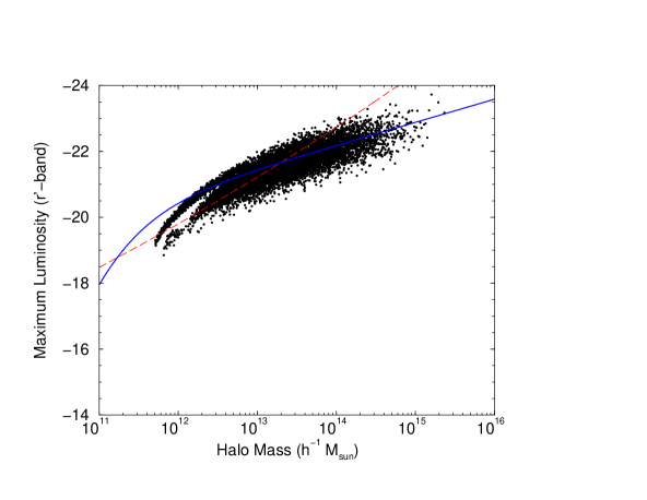
In Equation 1, $L_{c}(M,z)$ is the relation between central galaxy luminosity of a given dark matter halo and it’s halo mass, taken to be a function of the redshift, while $\sigma_{\rm cen}$, with a fiducial value of 0.17, is the log-normal dispersion in this relation. For an analytical description of the $L_{\rm c}(M,z)$ relation, we make use of the form suggested by Vale & Ostriker (2004) where this relation as appropriate for $b_{J}$-band galaxies today was established by inverting the 2dFGRS luminosity function given an analytical description for the sub-halo mass function of the Universe (e.g., De Lucia et al. 2004; Oguri & Lee 2004). The relation is described with a general fitting formula given by

$$L_{\rm c}(M,z)=L_{0}(1+z)^{\alpha}\frac{(M/M_{1})^{a}}{[b+(M/M_{1})^{cd(1+z)^{\eta}}]^{1/d}}\,.$$ (3)

For the rest B-band, the parameters have values of $L_{0}=5.7\times 10^{9}L_{\hbox{$\odot$}}$, $M_{1}=10^{11}M_{\hbox{$\odot$}}$, $a=4.0$, $b=0.57$, $c=3.72$, and $d=0.23$ (Vale & Ostriker 2004; Cooray 2005a,b), while for SDSS $r$-band, we take $M_{1}=2\times 10^{11}M_{\hbox{$\odot$}}$ and $c=3.78$ with other parameters as above. The redshift evolution of this relation, based on high-redshift LFs, is discussed in Cooray (2005b). Following the analysis described there, where we constrained values for redshift-dependent parameters $\alpha$ and $\eta$, we take fiducial values of -0.5 and -0.1; these were the best-fit parameters to the LFs of DEEP2 (Willmer et al. 2005), COMBO-17 (Bell et al. 2004), and rest B-band LFs of Gabasch et al. (2004).

Figure 6: Galaxy bias as a function of SDSS $r$-band absolute magnitude as calculated from CLFs (solid line) with SDSS bias measurements shown with data points (from Zehavi et al. 2004). We also separate contributions from central galaxies (dotted line) and satellites (dashed line) to galaxy bias. We also show the bias for galaxy types (early- and late-type galaxies). Late-type galaxies are expected to be in low-dense regions dominated by low-mass halos and their bias factor, relative to early type galaxies, would be lower. Satellite galaxies, regardless of the type, are in more massive halos and, thus, have higher bias factors relative to central galaxies. The average bias factor, shown here for the whole sample, however, is dominated by central galaxies due to the same reason that the LF is also dominated by central galaxies.

Figure 7: Projected correlation function of SDSS galaxies (from Zehavi et al. 2004). Left panel: For galaxies with $M_{r}<-20$. Here, we show the prediction based on CLFs and variations associated with a change in the power-law slope of the total luminosity–halo mass relation. For reference, we also show the projected clustering power spectrum from the linear power spectrum alone, but scaled by the large-scale bias factor for galaxies with same luminosities. Right panel: Clustering of galaxy types and cross-clustering between galaxy types for the sample with $M_{r}<-21$. For reference, we show both 2-halo and 1-halo contributions to the projected cross-correlation function between the two galaxy types.

Figure 8: Projected correlation function as a function galaxy absolute magnitude in the SDSS $r$-band (data from Zehavi et al. 2004). We show the predictions based on our fiducial model parameters. In addition to the total galaxy sample, when available, we also show the measurements, as well as predictions, for clustering of galaxy types. The CLFs associated with these predictions are shown in Fig. 3 while the halo occupation numbers, based on an integration of the CLFs, are shown in Figure 4.

For satellites, the normalization $A(M)$ of the satellite CLF can be obtained by defining $L_{\rm s}(M,z)\equiv L_{\rm tot}(M,z)-L_{\rm c}(M,z)$ and requiring that $L_{\rm s}(M,z)=\int_{L_{\rm min}}^{L_{\rm max}}\Phi^{\rm sat}(L|M,z)LdL$ with $g_{\rm s}(L)=1$, where the minimum luminosity of a satellite is $L_{\rm min}$. In the luminosity ranges of interest, and due to the numerical value chosen below for the slope $\gamma$, our CLFs are mostly independent of the exact value assumed for $L_{\rm min}$ as long as it lies in the range $(10^{6}-10^{8})L_{\hbox{$\odot$}}$. To describe the total luminosity of a halo, departing from the model used in Cooray (2005b), we make use of the following phenomenological form:

$$L_{\rm tot}(M,z)=\left\{\begin{array}[]{ll}L_{\rm c}(M,z)&M\leq M_{\rm sat}\\ L_{\rm c}(M,z)\left(\frac{M}{M_{\rm sat}}\right)^{\beta_{s}(z)}&M>M_{\rm sat}\end{array}\right.$$ (6)

Here, $M_{\rm sat}$ denotes the mass-scale at which satellites begin to appear in dark matter halos with luminosities as corresponding to those in the given sample of galaxies, while $\beta_{s}(z)$ is the correction to the power-law slope of the total luminosity–halo mass relation relative to that of the central galaxy–halo mass relation. We use this form since other parameterizations we considered resulted in unphysical situations for certain parameter values in those descriptions, e.g., $L_{\rm tot}(M)<L_{c}(M)$, while other parameterizations did not provide useful constraints on parameters used for the description due to additional degeneracies. More importantly, the above form allows us to highlight easily an interesting result, involving the single parameter best constrained by clustering data, that we will discuss later. When showing models of CLFs in Figures 3 to 8, motivated by constraints from that data that we will describe later, we take $M_{\rm sat}=10^{13}$ M${}_{\hbox{$\odot$}}$ and $\beta_{s}=0.55$ to describe $r$-band galaxies with absolute magnitudes $M_{r}<-17$. In Figures 11 and 12, same numerical values for the parameters of the satellite CLF are also used at high redshifts and in the rest B-band, though we note a redshift-dependent variation in these parameters, especially when considering $z=4$ clustering data from the Subaru Deep Field. Though we show figures with $M_{\rm sat}=10^{13}$ M${}_{\hbox{$\odot$}}$ and $\beta_{s}=0.55$, this does not mean these are the best-fit values or our preferred values for these parameters. When we model fit the data, we will show constraints on these parameters explicitly and show that a rather large range of values is allowed by the data. While these two parameters are degenerate with each other, in addition to SDSS data at $z<0.1$, certain high-redshift data, such as COMBO-17 at $z\sim 0.6$ and Subaru/XMM-Newton Deep Field with clustering measurements at $z\sim 4$, do allow constraints to be placed on these parameters.

While the above form refers to the total luminosity, when $L_{\rm tot}(M,z)>L_{\rm c}(M,z)$, this total luminosity must be distributed over a number of satellite galaxies in the halo when describing the satellite CLF. We take a power-law luminosity distribution and set $\gamma(M,z)=-1$ in Equation 1 based on previous results derived on the CLF of galaxy groups and clusters (Cooray & Milosavljević 2005b; Cooray 2005a) and direct measurement in clusters such as Coma (Driver & De Propis 2002 where $\gamma=-1.01^{+0.04}_{-0.05}$); While the choice of $\gamma\sim-1$ is motivated by the cluster LF, setting $\gamma$ to a different value between -0.7 and -1.3, over a set of parameter values we tested, did not change our results significantly. Furthermore, for the maximum luminosity of satellites in a given halo, following the result found in Cooray & Milosavljević (2005b) based on a comparison of predictions to the K-band cluster LF of Lin & Mohr (2004), we set $L_{\rm max}=L_{\rm c}/2$. A comparison to 2dFGRS CLFs as measured by Yang et al. (2005), however, suggested that such a sharp cut-off is inconsistent and that to account for scatter in the total galaxy luminosity, as a function of the halo mass, one must allow for a distribution in $L_{\rm max}$. Instead of additional numerical integrals, we allow for a luminosity dependence with the introduction of $g_{\rm s}(L)$ centered around the maximum luminosity of satellites such that $\Phi^{\rm sat}(L|M)$ does not go to zero rapidly at $L_{\rm max}$. By a comparison to the data, we again found a log-normal description with

$$g_{\rm s}(L)=\frac{1}{2}\left[1+{\rm erf}\left(\frac{\log(L_{\rm c}/2.0)-\log(L)}{\sigma_{s}}\right)\right]\,,$$ (7)

where $\sigma_{s}=0.3$. The description here is such that $f_{\rm L}=1$ when $L<L_{\rm mac}=L_{\rm c}/2$, but falls to zero at a luminosity beyond $L_{\rm c}/2$ avoiding the sharp drop-off at $L_{\rm c}/2$ with $g_{\rm s}(L)=1$. Again, our results are mostly insensitive to parameters of this description since variations here only lead to small changes to the overall CLF.

The central galaxy CLF takes a log-normal form while the satellite galaxy CLF takes a power-law form in luminosity. Such a separation describes the LF best with an overall better fit to the data in the K-band as explored by Cooray & Milosavljević (2005b) and 2dFGRS $b_{J}$-band in Cooray (2005). Our motivation for log-normal distribution also comes from measured galaxy cluster LFs that include bright central galaxies where a log-normal component, in addition to the Schechter (1976) form, is required to fit the data (e.g., Trentham & Tully 2002). Similarly, the stellar mass function as a function of halos mass in semi-analytical models is best described with a log-normal component for central galaxies (Zheng et al. 2004). As we find later the overall shape of the LF is strongly sensitive to the shape of the $L_{\rm c}$–$M$ relation, and it’s scatter, and less on details related to the $L_{\rm tot}$–$M$ relation. The non-linear part of the galaxy correlation function, or any clustering statistic, probes the satellite distribution and constraints can be put on the $L_{\rm tot}$–$M$ relation. In fact, we find that the average luminosity of satellites, defined in Section 4, is the single parameter best constrained with current data.

To describe galaxies as a function of color in this analytical description, we must further divide central and satellite galaxies as a function of their color given the luminosity. Here, motivated by the bimodality of color (e.g., Baldry et al. 2004) that extends out to high redshifts (e.g., Giallongo et al. 2005), we consider models in terms of galaxy types. The description in terms of galaxy types is also useful since measurements at high redshifts, so far, involve the division of galaxy samples to two broad categories involving early-type, or red, and late-type, or blue, galaxies. Thus, in the case of early type galaxies we write the CLF as

$$\Phi^{\rm cen}_{\rm early}(L|M,z) = \Phi^{\rm cen}(L|M,z)f_{\rm early-cen}(M,z)$$

$$\Phi^{\rm sat}_{\rm early}(L|M,z) = \Phi^{\rm sat}(L|M,z)f_{\rm early-sat}(M,L,z)\,,$$ (8)

where the two functions that divide between early- and late-types are taken to be functions of mass, in the case of central galaxies, and both mass and luminosity in the case of satellites. These functions are described analytically as

$$f_{\rm early-cen}(M,z)=$$ (9)

$$\frac{f_{\rm cen-E}(z)}{2}\left[1+{\rm erf}\left(\frac{\log(M)-\log(M_{\rm cen}(z))}{\sigma_{\rm early-cen}}\right)\right]\,,$$

with fiducial parameters of $M_{\rm cen}(z)=5\times 10^{11}$ M${}_{\hbox{$\odot$}}$, $\sigma_{\rm early-cen}=2.0$, and $f_{\rm cen-E}(z)=0.6$, and

$$f_{\rm early-sat}(M,L,z)=$$ (10)

$$g_{\rm sat-E}(z)g(M,z)+g_{\rm sat-E}(z)h(L,z)+f_{\rm sat-E}(z)\,,$$

where,

$$g(M,z) = \frac{1}{2}\left[1+{\rm erf}\left(\frac{\log(M)-\log(M_{\rm sat}(z))}{\sigma_{\rm sat}}\right)\right]$$

$$h(L,z) = \frac{1}{2}\left[1+{\rm erf}\left(\frac{\log(L)-\log(L_{\rm sat}(z))}{\sigma_{\rm sat}}\right)\right]\,,$$ (11)

with $M_{\rm sat}=10^{13}$ M${}_{\hbox{$\odot$}}$, $L_{sat}=3\times 10^{9}$ $L_{\rm sun}$, $\sigma_{\rm sat}=1$, $f_{\rm sat-E}(z)=0.4$ and $g_{\rm sat-E}(z)=0.2$; Early-type galaxies in the form of satellites varies from a fraction of $f_{\rm sat-E}(z)$ at low luminosity galaxies in low mass halos to $2g_{\rm sat-E}(z)+f_{\rm sat-E}(z)$ in halos with masses greater than $10^{13}$ M${}_{\hbox{$\odot$}}$. As fractions are defined with respect to the total galaxy number of a halo, late-type fractions are simply $[1-f_{\rm early-cen}(M,z)]$ and $[1-f_{\rm early-sat}(M,L,z)]$ for central and satellite galaxies, respectively and we do not need to specify there parameters separately.

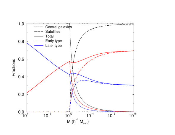
The fractions, following the fiducial values mentioned above — with some parameters estimated based on model fits to measurements described later — are shown in Fig. 1. The late-type fraction varies from $\sim$ 0.8 at halo masses of $10^{11}$ M${}_{\hbox{$\odot$}}$, in the form of central galaxies, to $\sim$ 0.3 when $M\sim 10^{15}$ M${}_{\hbox{$\odot$}}$ corresponding to galaxy cluster scales, with the fraction essentially dominated by satellite galaxies.

Figure 9: The three-dimensional cross-correlation function between galaxies and dark matter as determined by Sheldon et al. (2004) using SDSS galaxy-galaxy weak lensing measurements. The galaxy sample associated with this cross-correlation measurement a volume limited sample in redshifts between 0.1 and 0.174 and in magnitudes between $-23<M_{r}<-21.5$. The volume limited and luminosity-selected sample measurements allow an easy prediction based on the same fiducial parameters as those used to describe projected clustering measurements of galaxies. We also show the expected cross-correlation between mass and galaxy types. The dotted, dashed and dot-dashed lines show contribution from the central galaxy 1-halo term, the satellite galaxy 1-halo term and from linear theory, scaled by a bias factor, respectively.

Figure 10: Projected correlation function of galaxies at $z\sim 0.6$ as measured by the COMBO-17 survey (Phleps et al. 2005) and divided into clustering of early- and late-type galaxies. The predictions based on our fiducial model description, with appropriate parameters for redshift evolution of the $L_{\rm c}(M,z)$ relation, are also shown. In the case of early-type galaxies, we also show variations in the power-law slope of the total luminosity–halo mass relation. While not specified as part of the observations, we have assumed this sample corresponds to $M_{B}<-18$ when model fitting the data.

Figure 11: Projected correlation function of galaxies at $z\sim 1$ as measured by the DEEP2 survey (Coil et al. 2004). Left panel: Clustering of galaxies divided into two luminosity samples with $M_{B}<-19.75$ (circles) and $M_{B}>-19.75$ (squares). The predictions based on CLFs are also shown; We assume a low-end magnitude of -18 for the faint sample, while no such assumption is needed at the bright-end due to the cut-off associated with the LF. Right panel: Galaxy clustering in the total sample divided to galaxy types. In both panels, dotted lines are predictions based on the linear theory power spectrum.

Figure 12: Projected angular correlation function of galaxies at $z\sim 3$ as measured by the GOODS survey (Lee et al. 2005). The measurements are for the total sample, but for comparison, we also show the expected clustering of red- and blue-galaxies if the sample had been divided to galaxy types. For comparison, we also show the 1-halo contribution.

Figure 13: Projected angular correlation function of LBGs at $z\sim 4$ as measured in the Subaru/XMM-Newton Deep Field (Ouchi et al. 2005). Left panel: Clustering of galaxies with $i$-band magnitudes brighter than 27.5, corresponding to rest-frame $M_{B}<-18.5$. For comparison, we also show expected clustering with the same luminosity cut at $z\sim 5$ and 6; High signal-to-noise ratio clustering measurements at such high redshifts are soon expected from Subaru and other deep drop-out surveys. At high redshifts, large-scale clustering increases due to the evolution in the halo clustering bias factor, but at the same time, non-linear clustering decreases as the number of galaxies that appear as satellites at a given luminosity begins to decrease at high redshifts. The dotted line shows the prediction based on linear theory at $z\sim 4$, scaled by the large-scale bias factor for galaxies with $M_{B}<-18.5$ (see, Cooray 2005b). Right panel: Galaxy clustering at $z\sim 4$, divided to luminosity bins (measurements from Kashikawa et al. 2005 using the Subaru Deep Field data) as indicated on the figure. At each of these luminosity bins, we assume same parameters related to satellites as the ones used to describe clustering for the sample in the left panel. The differences in the one-halo non-linear term prediction and small-scale observed clustering are due most likely due to variations in the parameters related to the satellite CLF as a function of satellite luminosity. For example, with $M_{\rm sat}=5\times 10^{12}$ M${}_{\hbox{$\odot$}}$ and $\beta_{s}=0.6$, we over predict the small-scale clustering in the highest luminosity bin with $M_{B}<-20.5$, while small-scale clustering is well reproduced in the low luminosity bins. The excess in the high luminosity bin is due to the large number of satellites allowed, while a higher value for $M_{\rm sat}$ can be used to make the agreement with data better. This suggests that satellites with high luminosities appear in higher mass halos than compared to halos in which low luminosity galaxies appear; This is clearly consistent with the general expectation. A detailed analysis of luminosity dependent clustering at $z\sim 4$, using a new set of measurements from the imaging data in Ouchi et al. (2005), will be described in detail elsewhere (Cooray & Ouchi, in preparation).

3 Galaxy Luminosity Function

Given the CLF, the galaxy LF is obtained through

$$\Phi_{i}(L,z)=\int dM\,\frac{dn}{dM}(z)\,\Phi_{i}(L|M,z)\,,$$ (12)

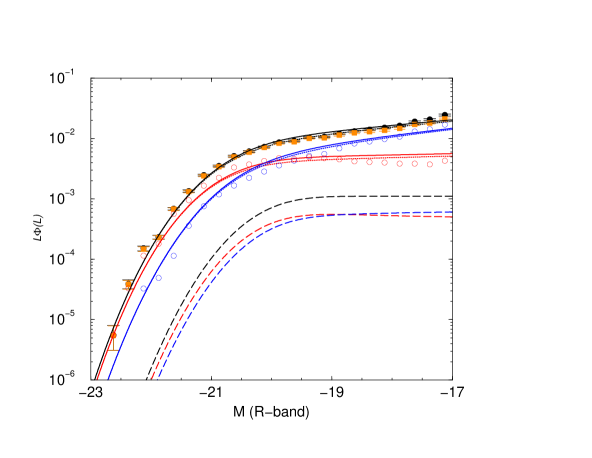
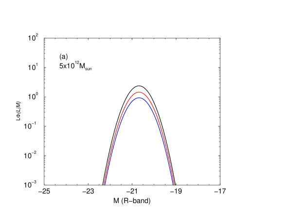
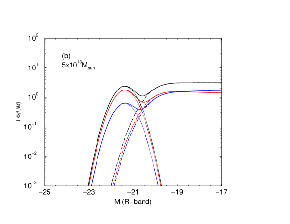
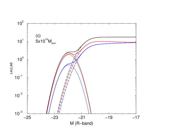
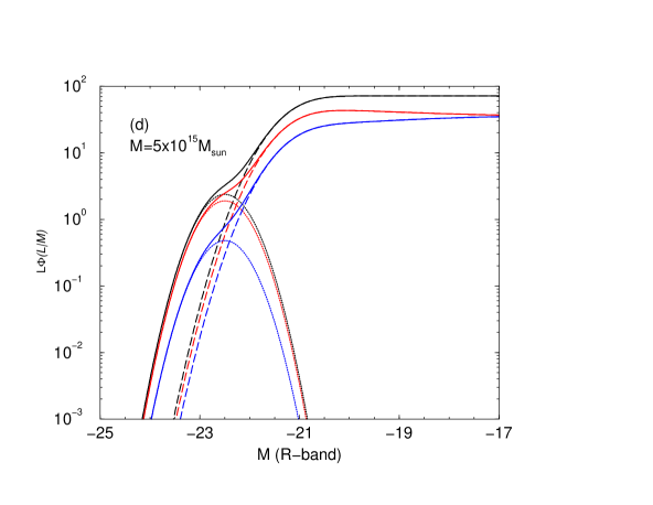
where $i$ represents the division to galaxy types. Here $dn/dM(z)$ denotes the mass function of dark matter halos and we use the formalism of Sheth & Tormen (1999) in our numerical calculations. This mass function is in better agreement with numerical simulations (Jenkins et al. 2001) when compared to the Press-Schechter mass function (Press & Schechter 1974). Using our fiducial values for CLF parameters, in Fig. 2, we show the SDSS galaxy LF (from Blanton et al. 2004) and the separation to early- and late-type galaxies. We only concentrate on galaxies with $M_{r}<-17$ since this sample overlaps with galaxies used by Zehavi et al. (2004) for clustering measurements that are also used in the present analysis. The CLFs related to this description are shown in Fig. 3. At the faint-end, these CLFs flatten due to our assumption that the power-law slope of the luminosity distribution within halos is $\gamma=-1$, which is consistent with the LF of galaxies in clusters over the magnitude range of interest to this paper. At fainter magnitudes the CLF becomes complicated due to effects associated with the luminosity distribution of dwarf galaxies (e.g., Cooray & Cen 2005). In the present analysis, we do not consider such low-luminosity galaxies with $M_{r}>-16$ and issues related to the subhalo mass function and associated substructure can therefore be easily ignored.

In previous discussions of galaxy clustering under the halo model the occupation number has been widely used as a way to relate statistics of dark matter to galaxies (e.g., Kauffmann et al. 1999; Benson et al. 2000; Berlind et al. 2003; see, review in Cooray & Sheth 2002). To compare with models of the halo occupation number, CLFs can be easily integrated such that

$$N_{\rm cen}(M,z) = \int dL\,\Phi^{\rm cen}(L|M,z)$$

$$N_{\rm sat}(M,z) = \int dL\,\Phi^{\rm sat}(L|M,z)\,.$$

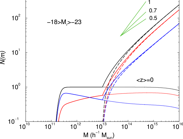
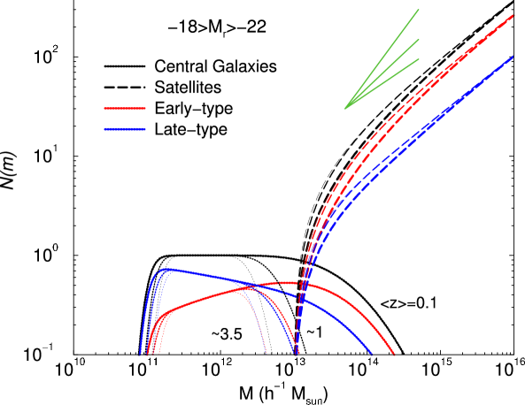
Since the halo occupation number captures no information on the luminosity distribution of galaxies, models involving the halo occupation number cannot be used to model the galaxy LF easily. We show the halo occupation number in Fig. 4 for $-23<M_{r}<-18$ galaxies in the SDSS sample (left panel) and redshift dependence of the halo occupation number (right panel). At high redshifts, the occupation numbers are at the B-band since galaxy samples in COMBO-17, DEEP2, and GOODS are defined at this wavelength. While Subaru/XMM-Newton Deep Field sample is defined in the observed $i$-band, we assume rest-frame B-band luminosities when model fitting the data.

In the case of satellites, since $N_{\rm sat}(M,z)=A(M,z)\int dL\,L^{\gamma(M)}f_{\rm s}(L)$ at the high mass limit of the halo mass with $\gamma(M)$ a constant and when $L_{\rm tot}(M,z)\gg L_{\rm c}(M,z)$ we expect $N_{\rm sat}(M)\propto L_{\rm tot}(M,z)\sim M^{\beta_{s}+\alpha}$, where $\beta_{s}$ is the slope introduced in equation 4 and $\alpha$ is the slope of the $L_{c}(M)$ relation at the same halo masses. With $\alpha_{s}\sim 0.2$, and $\beta_{s}=0.55$, the fiducial slope of occupation number is around 0.75, though this slope is mass dependent given the rapid variation of central galaxy luminosity with halo mass.

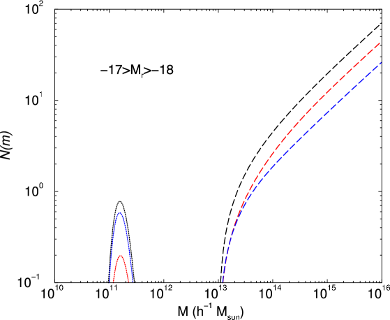
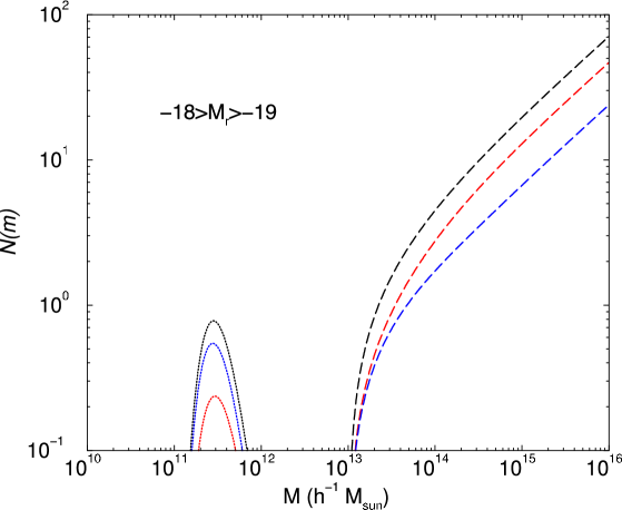
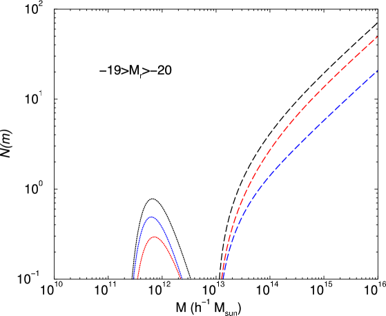
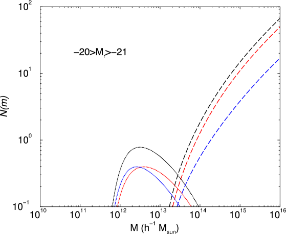
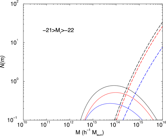
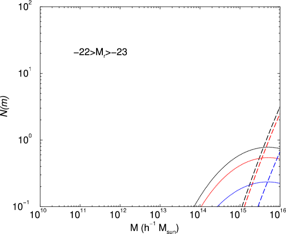
In Fig. 5, we present the halo occupation number as a function of luminosity considered by Zehavi et al. (2004) for clustering measurements. These occupation numbers, based on CLFs, can be compared with best-fit halo occupation models suggested in Zehavi et al. (2004). In our fiducial model, satellites with $M_{r}<-17$ only appear in halos with masses greater than $M_{\rm sat}=10^{13}$ M${}_{\hbox{$\odot$}}$. We see a cut-off in the halo occupation number of central galaxies at masses around $10^{11}$ M${}_{\hbox{$\odot$}}$. At $M_{r}<-20$, this cut-off is around $\sim 7\times 10^{11}$ M${}_{\hbox{$\odot$}}$. This value can be compared to the suggested minimum value of $\sim 10^{12}$ M${}_{\hbox{$\odot$}}$ for the halo occupation number down to the same magnitude in Zehavi et al. (2004). The difference can be understood based on the fact that Zehavi et al. (2004) description of the satellite halo occupation number is $(M/M_{1})^{\alpha}$ with a no cut-off at a lower mass, while the minimum halo mass cut-off only applies to the central galaxy occupation number. It could be that the degeneracy between the central and satellite galaxy occupation numbers leads to an overestimate in the minimum mass for central galaxies to appear, while that overestimate is partly accounted with an increase in the slope of the halo occupation number for satellite galaxies.

As stated in Zehavi et al. (2004), the halo occupation model parameters suggested there are not unique. The mass cut-off detected based on the halo occupation number model fits to galaxy statistics should not be treated as a general lower limit on halo mass to host galaxies. The cut-off usually one detects with occupation numbers is the minimum halo mass to host a galaxy given the minimum luminosity of galaxies in the sample under consideration (for example, the minimum mass of the central galaxy halo occupation number as a function of luminosity in Fig. 5). It could be that halos with a mass lower than the cut-off continue to host galaxies, but with a lower luminosity, and due to sample selection criteria such halos would not be included in the sample used for clustering studies. We will return to this below in the context of model fits to clustering data where we find no conclusive evidence for a general minimum halo mass to host galaxies, for galaxies with $M_{r}<-17$.

In addition to the low mass cut-off of central galaxies, we also have the freedom to select a low mass for the appearance of satellites with the parameter $M_{\rm sat}$. In Figures 4 and 5, we have set $M_{\rm sat}=10^{13}$ M${}_{\hbox{$\odot$}}$, though best-fit halo occupation numbers from Zehavi et al. (2004) suggest the presence of satellites, as appropriate for the same sample of galaxies, in halos with a lower mass than this. While this could be due to differences between the model, as stated before, the occupation models as well as our CLFs may not be unique. Later, we will use data to constrain parameters such as $M_{\rm sat}$ and find large degeneracies between $\beta_{s}$, the power-law slope, and $M_{\rm sat}$ such that as $M_{\rm sat}$ is lowered, $\beta_{s}$ is increased. The same degeneracy should also appear in model fits based on the halo occupation number. For example, with a larger value for M_min, the minimum mass for the central galaxy halo occupation number as in model descriptions of Zehavi et al. (2004), one should find a larger slope $\alpha$ for the satellite halo occupation number such that the total number of satellite galaxies remains the same; This behavior could partly explain the unusually large values for the slope suggested in Zehavi et al. (2004). The degeneracy between $M_{\rm sat}$ and $\beta_{s}$ suggests that a single parameter involving the combination of these two parameters can be best determined with the data. As we find later, this parameter is the total luminosity of satellite galaxies averaged over the halo mass distribution that hosts galaxies between $-17>M_{r}>-23$ in the SDSS sample.

Figure 14: Constraints on parameters $\sigma_{\rm cen}$, the log-normal dispersion of the central galaxy—halo mass relation, and $M-{\rm cen-cut}$, the lower halo mass to host a central galaxy, independent of luminosity, related to the central galaxy CLF description. The left panel shows the constraint based on the SDSS LF (from Blanton et al. 2004), down to $M_{r}$ of -17, and the right panel shows the constraints from SDSS galaxy clustering measurements (from Zehavi et al. 2004). While the LF strongly constrains these parameters, clustering measurements do not. The difference comes from the fact that clustering measurements are more sensitive to satellite galaxies while, as shown in Figure 2, LF measurements are sensitive to statistics of central galaxies.

Figure 15: Constraints on parameters $f_{\rm cen-E}$, the fraction of early-type central galaxies at the high mass-end and $M_{\rm cen}$ related to the analytical description of the early-type galaxy fraction of central galaxies. The left panel shows the constraint based on SDSS galaxy type LFs (from Blanton et al. 2004), down to $M_{r}$ of -17, and the right panel shows the constraints from SDSS galaxy clustering measurements divided to galaxy types between magnitudes bins from -18 to -21 (from Zehavi et al. 2004). As above, while LF strongly constrain parameters related to central galaxies clustering measurements do not.

                

Figure 16: Constraints on parameters that describe galaxy types related to the satellite CLF (see, equation 6) based on galaxy clustering data divided to galaxy types between $-18>M_{r}>-22$ in SDSS. While M_sat is not strongly constrained with clustering data, $f_{\rm sat-E}$ describing the fraction of early type galaxies as satellites in low mass halos is constrained to be between 0.5 $\pm 0.15$ at the 68% confidence level. The right-panel shows constraints on parameters $f_{\rm sat-E}$ and $g_{\rm sat-E}$.

         

         

Figure 17: Constraints on parameters $\beta_{\rm s}$, the additional power-law slope of total luminosity–halo mass relation (in addition to the slope of central galaxy–halo mass relation), and $M_{\rm sat}$, the halo mass scale at which satellites begin to appear, related to the satellite CLF. These constraints come from clustering measurements from SDSS (top left), COMBO-17 (top right), DEEP2 (middle left), GOODS (middle right), and Subaru/XMM-Newton Deep Field (bottom panel) at redshifts less than 0.1, around 0.6, around unity, between 2.5 and 3.5, and at 4, respectively. We only make use of total clustering data divided to galaxy luminosity bins here, but the constraints shown above are for the combine data set at each of the redshifts. In later figures, we will highlight differences between certain luminosity bins instead of the overall constraint shown here.

Figure 18: $\langle L_{\rm sat}\rangle$, the sample-averaged luminosity of satellites for the given sample of galaxies (equation 4), as a function of $\beta_{\rm s}$, the power-law slope of total luminosity–halo mass relation, and $M_{\rm sat}$, the halo mass scale at which satellites appears. The dashed lines show the average satellite luminosity for SDSS sample while dotted lines show the same at $z\sim 3$ as appropriate for the GOODS survey. For reference, we overlap constraints on this parameter space from SDSS (same as Figure 17, top left panel). The degeneracy in $\beta_{s}$–$M_{\rm sat}$ plane traces contours of equal average satellite luminosity and this single parameter is best constrained by current galaxy clustering measurements.

         

Figure 19: Left panel: $\langle L_{\rm sat}\rangle$, the sample-averaged luminosity of satellites as a function of $\beta_{\rm s}$ and $M_{\rm sat}$ at $z=4$ for galaxies with $M_{B}<-18.5$. For reference, we overlap constraints on this parameter space from Subaru (same as Figure 19, bottom panel). Right panel: $\bar{n}(z)$, the number density of galaxies at $z\sim 4$ with $M_{B}<-18.5$, as a function of as a function of $\beta_{\rm s}$, the power-law slope of total luminosity–halo mass relation, and $M_{\rm sat}$, the halo mass scale at which satellites appears (in units of $10^{-3}$ h${}_{70}^{3}$ Mpc^-3). For reference, we overlap constraints on this parameter space from Subaru/XMM-Newton Deep Field (same as Figure 17, bottom panel). The degeneracy in $\beta_{s}$–$M_{\rm sat}$ plane also traces essentially contours of equal number density of galaxies as well as equal values for $\langle L_{\rm sat}\rangle$.

         

Figure 20: Constraints on parameters $\beta_{\rm s}$, the additional power-law slope of total luminosity–halo mass relation (in addition to the slope of central galaxy–halo mass relation), and $M_{\rm sat}$, the halo mass scale at which satellites begi n to appear, related to the satellite CLF from Subaru/XMM-Newton Deep Field at $z=4$ compared with constraints from SDSS (left panel) and COMBO-17 (right panel). At the 1$\sigma$ confidence, a clear difference between constraints at $z\sim 4$ and at $z\sim 0.6$ is clear. In the text, we discuss this difference in the context tha t we find no difference in the redshift dependence of $\langle L_{\rm sat}\rangle$.

Figure 21: The constraints on $M_{\rm sat}$–$\beta_{s}$ plane at two different luminosity bins: dotted lines show the constraint when $-18>M_{r}>-19$ and solid lines show the case for $-21>M_{r}>-22$. We find some evidence for an increase in $M_{\rm sat}$ as the galaxy luminosity is increased, but the exact dependence between $M_{\rm sat}$ and galaxy luminosity is not well established with current data.

Figure 22: Left: The minimum mass for the appearance of satellite galaxies at a given luminosity as a function of the halo mass based on a catalog of galaxy groups and clusters in the SDSS (described in Weinmann et al. 2005). Here, each data point represents a group or a cluster where the the halo mass was determined based on the total luminosity of the halo. Each data point represents the luminosity of the faintest galaxy assigned to each halo. Here, we focus on the $r^{\prime}$-band luminosity as the sample used for galaxy clustering in Zehavi et al. (2004) is defined for that sample. The solid line shows the relation established from this catalog between the minimum luminosity in the $r^{\prime}$-band and the halo mass: $M_{r}(min)\approx-19.8(M/10^{12}\;M_{\hbox{$\odot$}})^{0.03}$. Right: The maximum luminosity of a halo as a function of the halo mass. Here, we plot the luminosity of the brightest galaxy assigned to that halo (which may or may not the central galaxy in terms of cluster/group dynamics). The long-dashed line is the same relation as that in the left panel. The solid line is the relation between central galaxy luminosity and the halo mass as described in equation (3) at $z=0$ as required to explain the SDSS luminosity function from Blanton et al. (2004). The mass estimate is highly uncertain when halo masses are below few times 10¹² M${}_{\hbox{$\odot$}}$ due to the small number of galaxies and the scatter in the luminosity of the dominant galaxy. Due to this, and the uncertain assignment of galaxies that are satellites of a bigger halo to less massive halos, we do not consider the difference at the low mass end between the brightest galaxy luminosity and the expected luminosity from the $L_{c}(M)$ relation to be any concern.

       

       

Figure 23: Fraction of satellites as a function of the luminosity bin in $r$-band, as labeled on each of the four panels, as a function of $\beta_{\rm s}$, the power-law slope of total luminosity–halo mass relation, and $M_{\rm sat}$, the halo mass scale at which satellites appears. For reference, we overlap the constraints on this parameter space from SDSS as relevant for each of the luminosity bins; Note that these constraints are worse than the overall constraint on this plane when the galaxy sample is combined. Satellite fractions range from 0.05 to 0.15, when $-22<M_{r}<-21$ to $\sim 0.1$ to 0.5 when $-19<M_{r}<-18$ at the 68% confidence level. These fractions are consistent with values suggested in Mandelbaum et al. (2004) in the three low-luminosity bins based on an analysis of galaxy-galaxy lensing data with numerical simulations.

Figure 24: Probability distribution for the fraction of satellites as a function of the luminosity bin in $r$-band, as labeled on each on the left panel. Left panel: Satellite fraction with $\beta_{s}$ taken as a uniform prior between 0 and 1. Right panel: Satellite fraction with the constraint that $0.4<\beta_{s}<1$. The lower estimate was taken to be roughly consistent with the minimum luminosity—halo mass relation suggested by the SDSS galaxy group catalog data (Fig. 22), combined with clustering constraints shown in Fig. 21 and 23.

Figure 25: The conditional probability distribution function of halo mass $P(M|L,z)$ to host a galaxy of the given luminosity and at the given redshift as a function of the halo mass. The black lines are the total galaxy sample while red and blue lines show the sample divided to early- and late-type galaxies. Left- and right-panels show these probabilities for $M_{r}$ or $M_{B}$ magnitudes between -18 and -19, and between -22 and -23, respectively at redshifts of 0.1 (in r-band), 3 and 5 (in B-band), in decreasing thickness of lines.

Figure 26: The conditional probability distribution function of halo mass $P(M|L,z)$ to host a galaxy of the given luminosity at a given redshift as a function of the halo mass. The four panels show these probabilities at different redshifts as labeled on each of the panels, while the plotted curves are for magnitudes between [-19,20], [-20,-21] and [-21,-22], in r-band at a redshift of 0.1 and B-band for other redshifts, with probabilities shown separately for central (dotted lines) and satellite (dashed lines) galaxies. These probabilities based on CLFs can be compared with the same probabilities extracted from an analysis of SDSS galaxy-galaxy lensing data in Mandelbaum et al. (2004; see, their figures 3 and 4) using numerical simulations.

Figure 27: The predicted cross-correlation between SDSS faint and bright samples of galaxies. For comparison we show the clustering of galaxies in each of the luminosity bins (from Zehavi et al. 2004), but cross-clustering between luminosity bins is yet to be measured. We propose such a measurement as a way to improve constraints on parameters related to the satellite CLF of the fainter sample. In addition to cross-clustering between galaxies in separate luminosity bins one can also consider cross-clustering between galaxy types (shown as the upper dot-dashed line for clustering between early type galaxies in the brighter sample and late-type galaxies in the fainter sample). A complete set of such measurements across several luminosity bins, in the form of a covariance matrix of cross-correlations $C(L_{a}^{i},L_{b}^{j},r)$, will provide all the information related to galaxy clustering at the two-point level and will provide additional information to constrain parameters related to the galaxy type CLFs.

4 Galaxy Clustering with CLFs

Using the CLF, instead of the halo occupation number, we can write the power spectrum of galaxies between type $i$ and type $j$ in terms of the 1- and 2-halo terms (see, review in Cooray & Sheth 2002) at a redshift $z$ as

$$P_{\rm gal}^{ij}(k|L,z)=P^{ij}_{1h}(k|L,z)+P^{ij}_{2h}(k|L,z)\,,\qquad{\rm where}$$ (14)

$$P^{ij}_{1h}(k|L,z)=\frac{1}{\bar{n}_{i}(L,z)\bar{n}_{j}(L,z)}\int dM\,\frac{dn(z)}{dM}$$

$$\times \Big{[}\Phi_{i}^{\rm sat}(L|M,z)\Phi_{j}^{\rm sat}(L|M,z)u^{2}_{\rm gal}(k|M,z)$$

$$+ \Phi_{i}^{\rm cen}(L|M,z)\Phi_{j}^{\rm sat}(L|M,z)u_{\rm gal}(k|M,z)$$

$$+ \Phi_{j}^{\rm cen}(L|M,z)\Phi_{i}^{\rm sat}(L|M,z)u_{\rm gal}(k|M,z)\Big{]}$$

$$\quad\quad{\rm and}$$

$$P^{ij}_{2h}(k|L,z)=P(k,z)\Big{[}I^{\rm cen}_{i}(k|L,z)I^{\rm cen}_{j}(k|L,z)$$

$$+ I^{\rm cen}_{i}(k|L,z)I^{\rm sat}_{j}(k|L,z)+I^{\rm sat}_{i}(k|L,z)I^{\rm cen}_{j}(k|L,z)$$

$$+ I^{\rm sat}_{i}(k|L,z)I^{\rm sat}_{j}(k|L,z)\Big{]}$$

with the integrals $I^{\rm cen}(k|L,z)$ and $I^{\rm sat}(k|L,z)$ given by

$$I^{\rm cen}_{i}(k|L,z)=\int dM\,\frac{dn(z)}{dM}b_{1}(M,z)\frac{\Phi_{i}^{\rm cen}(L|M,z)}{\bar{n}_{i}(L,z)}\quad{\rm and}$$

$$I^{\rm sat}_{i}(k|L,z)=\int dM\,\frac{dn(z)}{dM}b_{1}(M,z)\frac{\Phi_{i}^{\rm sat}(L|M,z)}{\bar{n}_{i}(L,z)}u_{\rm gal}(k|M,z)\,,$$

respectively. Here, and above,

$$\bar{n}_{i}(L,z)=\int dM\,\frac{dn(z)}{dM}\,\left[\Phi_{i}^{\rm cen}(L|M,z)+\Phi_{i}^{\rm sat}(L|M,z)\right]$$ (16)

denotes the mean number density of galaxies of type $i$ while

$$u_{\rm gal}(k|M,z)=\int_{0}^{r_{vir}}dr\ 4\pi r^{2}\,{\sin kr\over kr}\ {\rho_{\rm gal}(r|M,z)\over M}\,,$$ (17)

denotes the normalized Fourier transform of the galaxy density distribution within a halo of mass $M$ when $b_{1}(M,z)$ is the first-order bias factor of dark matter halos. Here for dark matter halo bias we use the bias factor derived by Sheth, Mo & Tormen (2001) which corrects earlier calculations by Mo et al. (1997; Efstathiou et al. 1988; Cole & Kaiser 1989) based on spherical collapse arguments.

The standard assumption in above equations is that galaxies trace dark matter within halos such that one can utilize the dark matter distribution given by analytic forms such as the NFW (Navarro et al. 1996) profile. An improved approximation will be to use the density distribution defined by sub-halos to describe galaxies and, instead of the halo mass function, use a combination of halo mass function and the subhalo mass function to describe the satellite contribution to galaxy clustering that also accounts for effects associated with substructure (e.g., Sheth & Jain 2002). Even if corrections exist for the power spectrum from the subhalo mass function, these only modify the strongly non-linear regime and leave the transitional regime from linear to non-linear clustering probed by current galaxy clustering measurements unaffected. Since relevant profiles related to substructure is still not well studied numerically we make use of the NFW dark matter density profile (Navarro et al. 1997) to describe the galaxy distribution within halos. The concentration parameter is defined following the scaling relation of Bullock et al. (2001). The relevant expressions in our calculation are summarized in Cooray & Sheth (2002). In a future paper we plan to combine galaxy-galaxy lensing measurements with galaxy clustering measurements to test the extent to which galaxies trace dark matter. For now, we will ignore any differences in the galaxy profile relative to dark matter and concentrate only on basic parameters related to the CLF rather than statistics such as profiles.

In Equation 14, when $i=j$, the expression reduces to the power spectrum of galaxies of the same galaxy type. Similarly one can ignore the index $i$ and $j$ and replace the CLF with the total CLF to calculate the power spectrum of the total galaxy sample at a given luminosity. Furthermore, one can also consider the cross power spectrum of samples between $(L_{1},i)$ with $(L_{2},j)$, where $i$ and $j$ denote the type, but instead of at a fixed luminosity, cross-correlations are considered between different luminosities. In this case, the above expressions must be generalized for the case with two different luminosity bins. Since this is straightforward, we do not reproduce the appropriate expressions here. These cross-correlation measurements between two different luminosity bins and different galaxy types across those bins are yet to be measured. These measurements provide the full set of clustering measurements related to galaxies and can be thought of as a covariance matrix of the form $C(L_{a}^{i},L_{b}^{j},r)$ where $a$ and $b$ are indices over the luminosity bins and $i$ and $j$ are indices over the galaxy types, while $r$ is the projected length at which clustering is measured. Towards the end of our discussion, we will motivate such a full set of measurements as a way to establish the satellite CLF more accurately.

For reference, to compare with lensing-lensing galaxy measurements, the cross-power spectrum between galaxies of type $i$ and the dark matter distribution is

$$P_{\delta-i}(k|L,z)=P^{\delta-i}_{1h}(k|L,z)+P^{\delta-i}_{2h}(k|L,z)\,,\qquad{\rm where}$$ (18)

$$P^{\delta-i}_{1h}(k|L,z)=\frac{1}{\bar{n}_{i}(L,z)}\int dM\,\frac{M}{\bar{\rho}}\frac{dn(z)}{dM}$$

$$\times \Big{[}\Phi_{i}^{\rm sat}(L|M,z)u^{2}_{\rm gal}(k|M,z)$$

$$+ \Phi_{i}^{\rm cen}(L|M,z)u_{\rm gal}(k|M,z)\Big{]}$$

$$\quad\quad{\rm and}$$

$$P^{\delta-i}_{2h}(k|L,z)=P(k,z)\Big{[}I^{\rm cen}_{i}(k|L,z)I^{\delta}(k,z)$$

$$+ I^{\rm sat}_{i}(k|L,z)I^{\delta}(k,z)\Big{]}$$

with the integral $I^{\delta}(k,z)$ given by

$$I^{\delta}(k,z) = \int dM\,\frac{M}{\bar{\rho}}\frac{dn(z)}{dM}b_{1}(M,z)u_{\rm gal}(k|M,z)\,,$$ (19)

and $\bar{\rho}$ is mean comoving density of dark matter.

At large scales, the galaxy power spectrum or the cross-power spectrum, reduces to that of the linear power spectrum scaled by the constant galaxy bias factor(s). One can understand this by noting that at large scales, $u_{\rm gal}(k|M,z)\to 1$ and the galaxy power spectrum simplifies to

$$P_{{\rm gal}}(k|L,z)\approx b_{i}(L,z)b_{j}(L,z)\,P(k,z),$$ (20)

where

$$b_{i}(L,z)=$$ (21)

$$\int dM\,\frac{dn(z)}{dM}\,b_{1}(M,z)\,\frac{\left[\Phi_{i}^{\rm cen}(L|M,z)+\Phi_{i}^{\rm sat}(L|M,z)\right]}{\bar{n}_{i}(L,z)}\,,$$

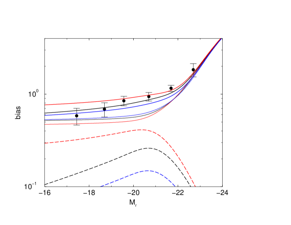
is the mean large-scale bias factor of the $i$-type galaxy population. This large-scale bias factor has already been discussed using CLFs previously (see, Cooray & Milosavljević 2005b; Cooray 2005a,b) and we summarize results based on the current analysis in Fig. 6.

Given the power spectrum, the three-dimensional correlation function of galaxies of type $i$ and $j$ with luminosity $L$ at a redshift of $z$ is

$$\xi_{ij}(r|L,z)=\int\frac{k^{2}dk}{2\pi^{2}}P_{ij}(k|L,z)\frac{\sin(kr)}{kr}\,.$$ (22)

Given limited statistics, most measurements are averaged over samples of galaxies distributed over a certain redshift range. In this case the projected correlation function follows as

$$w_{p}^{ij}(r|L,z)=\int\frac{kdk}{2\pi}P_{ij}(k|L,z)J_{0}(kr)\,.$$ (23)

In the case of a broad redshift distribution of galaxies over which clustering is projected the same correlation function is generally written in terms of angular scale, $\theta$, with the correspondence $r=\theta d_{A}$, where $d_{A}$ is the comoving angular diameter distance. To calculate such a broad correlation function in redshift space, we average over the galaxy redshift distribution associated with clustering measurements such that

$$w_{p}^{ij}(\theta|L,z)=\int drn^{2}(r)\int\frac{kdk}{2\pi}P_{ij}(k|L,z)J_{0}(kd_{A}\theta)\,,$$ (24)

where $n(r)$ is the normalized radial distribution of galaxies with $\int drn(r)=1$.

In our model predictions we calculate the projected correlation function at the mid point of the redshift distribution of galaxies used in that sample. The measurements where the exact redshift distribution plays an appreciable role is those of the GOODS survey (Lee et al. 2005) and the Subaru Deep Field (Ouchi et al. 2005) since galaxies are broadly distributed over a wide range in redshift from 2.5 to 4.5 and from 3.5 to 4.5, respectively. Fortunately, for both these surveys the expected redshift distribution of galaxies is known either through Monte Carlo simulations, in the case of GOODS (Lee et al 2005), or, in the case of Subaru Deep Field, through a combination of spectroscopic redshift measurements and Monte Carlo estimates (Ouchi, private communication). We take these distributions into account when model fitting GOODS and Subaru $w_{p}(\theta)$ measurements.

Another uncertainty in some of these measurements is the exact luminosity distribution of galaxies in the sample. For surveys such as SDSS and DEEP2 galaxy luminosities are a priori known and samples are binned in luminosity, while for surveys such as GOODS and Subaru Deep Field, the exact luminosity distribution remains uncertain, though statistics in terms of the apparent magnitude at the observed wavelength. As appropriate, given the redshift information, we converted some of the suggested apparent magnitudes of galaxies in the sample to rest-frame luminosities at the observed wavelength, usually in the rest B-band, and used that information to establish the minimum luminosity of galaxies in the sample. The minimum luminosity usually plays a larger role while the maximum luminosity of galaxies in the sample does not due to the bright-end exponential cut-off in the galaxy LF.

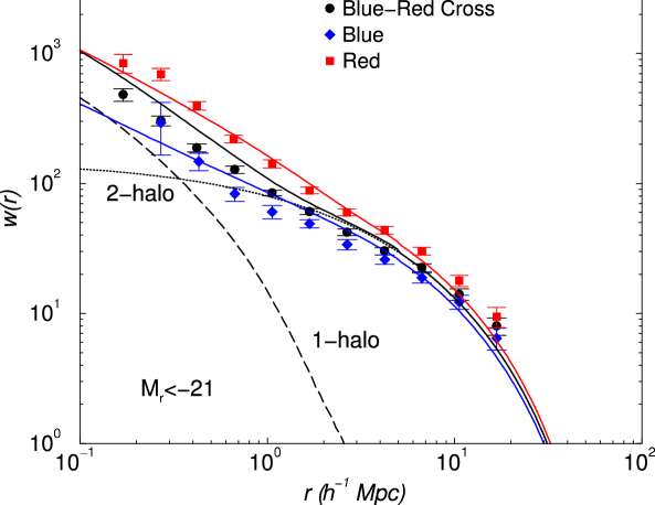
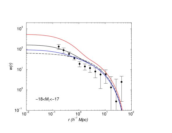
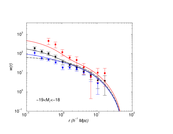
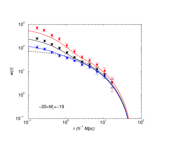
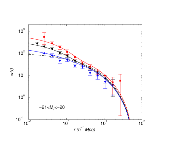
In Fig. 7, we show the projected correlation function of SDSS galaxies with $M_{r}<-20$ from Zehavi et al. (2004) and a comparison to model predictions based on the CLF using the fiducial description of model parameters. The corresponding CLFs of these model fits are in Fig. 5. For reference, Fig. 7 left panel illustrates the dependence of projected correlation function when the power-law slope of the total luminosity-halo mass relation is varied with $M_{\rm sat}$ fixed at the same fiducial value. In general, an increase in $\beta_{s}$ can be compensated by an increase in $M_{\rm sat}$. This degeneracy will become clear when we study model fits to the data later. In the right panel of Fig. 7, we illustrate the projected correlation function of galaxy types as well as the cross-correlation between two galaxy types with $M_{r}<-21$. The presence of a non-linear part for the cross-correlation between galaxy types can be easily understood based on the fact that both early- and late-type exists in similar mass halos (Zehavi et al. 2004).

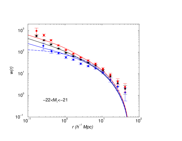
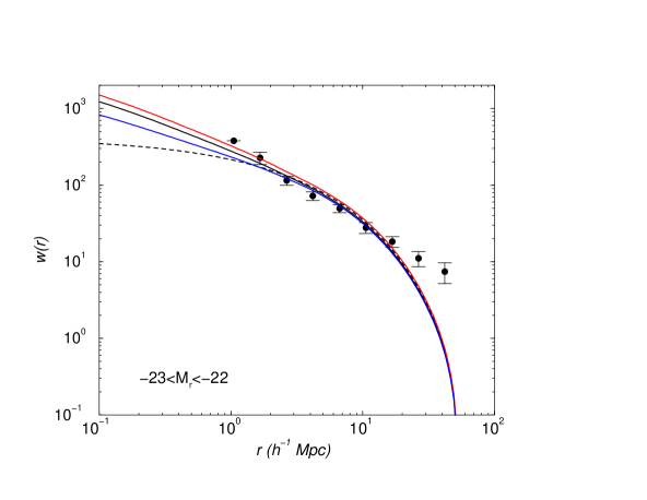
In Fig. 8, we summarize the projected correlation function as a function of luminosity bins considered by Zehavi et al. (2004); For the faintest (-17 to -18) and the brightest (-22 to -23) bin, only the total clustering correlation function is measured, though for comparison, we continue to show the clustering correlation function for both early- and late-type galaxies. Note that with our fiducial model parameters, measured projected correlation functions in magnitude bins between -19 to -20, -20 to -21, and -21 to -22 are generally well described, while fits are generally less than perfect in both the low luminosity and high luminosity bins. This is due to the fact that our fiducial model parameters are extracted from an overall fit to the whole sample assuming the same underlying description for the CLF for the whole galaxy sample. When model fitting the data, since measurements in mid magnitude bins are better determined, the fits are weighted more for these bins than ones at the two ends. We did not attempt to weight different bins equally. At this initial stage of analysis we are mostly interested in extracting a consistent model for the overall CLF of galaxies from current measurements or trying to understand the extent to which data can constrain parameters related to the CLF. The models considered in Zehavi et al. (2004) involved different occupation number descriptions for different luminosity bins. The CLF approach avoids having to describe occupation numbers separately for different luminosity bins, though it is likely and, guaranteed to be, that some parameters such as $M_{\rm sat}$ will be luminosity dependent, though parameters such as $\beta_{s}$ should not be. We will also show results where we model fitted the data separately based on divisions to luminosity bins. While the overall fits are not strong, we do find certain limited evidence for variation in $M_{\rm sat}$ as a function of the luminosity. While the CLF description leads to a certain reduction in the number of parameters to be determined from data, though we note that, due to our introduction of new parameters involving galaxy types etc, there is in fact no reduction but rather an increase in parameters. Later, in the discussion, we will propose additional measurements related to the same sample of galaxies in SDSS as Zehavi et al. (2004) and these measurements could further aid in improving model fits to determine current parameters better.

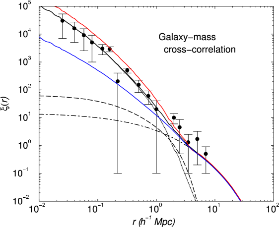
To show that our models are consistent, in Fig. 9, we compare our prediction for the galaxy-mass cross-correlation function, in real space, for a volume limited sample with $-21.5>M_{r}>-23$, and in the redshift range between 0.1 and 0.174. This galaxy sample has been used by Sheldon et al. (2004) to make a measurement of the galaxy-mass cross-correlation function via galaxy-galaxy weak lensing measurements in SDSS. We find our predictions agree well with measurements, and as a further application, in Fig. 9, we also show the expected cross-correlation if the foreground galaxy sample of Sheldon et al. (2004) had been further divided to blue- and red-galaxies, following essentially the same division to galaxy types as in Zehavi et al. (2004).

In Cooray & Milosavljević (2005a) we made use of SDSS galaxy-galaxy weak lensing measurements in the z’-band to construct $L_{c}(M)$ relation at higher wavelengths. These measurements are analyzed using the halo model in a variety of studies (e.g., Mandelbaum et al. 2004; Guzik & Seljak 2002; Yang et al. 2003a; Sheldon et al. 2004) and we do not make use of the galaxy-mass correlation function when model fitting parameters here. This is due to the fact that we are primarily interested in understanding the extent to which CLFs can be constructed from galaxy clustering measurements and to check our estimates, say, on the halo mass of galaxies at a given luminosity from estimates made by prior studies using galaxy-galaxy lensing measurements. We do this in the context of probability distribution for halo mass at a given galaxy luminosity (Mandelbaum et al. 2004).

The approach based on CLFs easily allows us to model clustering statistics at high redshifts within the same parameter description provided that redshift dependences are properly taken into account. Given the results from Cooray (2005b) on the redshift evolution of the $L_{c}(M)$ relation, here we take the redshift dependence of the central galaxy luminosity with redshift into account with parameters $\alpha$ and $\eta$ in equation 5. For parameters in the satellite CLF, such as $\beta_{s}$ and $M_{\rm sat}$, we do not attempt to include redshift variations given the lack of knowledge. On the other hand, redshift dependences can be extracted by analyzing clustering measurements as a function of redshift and by looking for differences in parameters constrained at different redshifts. This was the approach used in Cooray (2005b) to establish redshift variation in $L_{c}(M)$ relation.

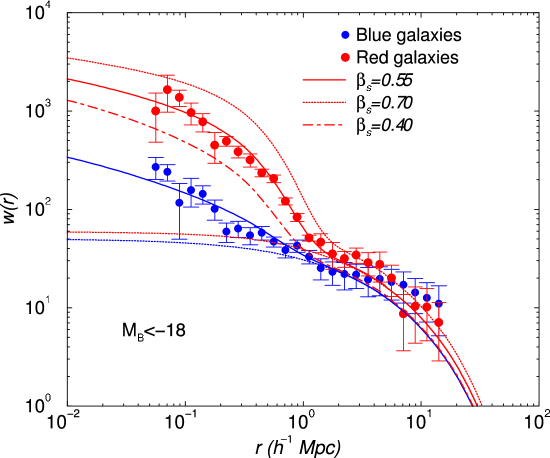
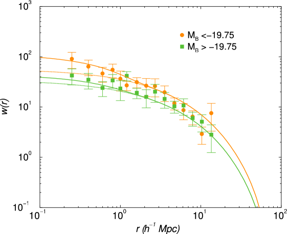
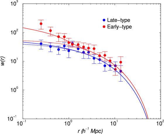
In Fig. 10, we compare our predictions for projected galaxy clustering at redshifts 0.4 to 0.8 as determined by the COMBO-17 survey (Phleps et al. 2005). These data involve rest B-band magnitudes and we make use of the $L_{c}(M)$ relation as appropriate for rest B-band from Cooray (2005b) including the redshift evolution with parameters described with respect to equation 3. While our fiducial parameters describe the non-linear clustering part of early- and late-type galaxies in this sample well, we find that large-scale clustering of late-type galaxies is not modeled by our parameters. We find the same difference between measurements and model fits based on the halo occupation number appears in the analysis by Phleps et al. (2005) as well. We use this data set to extract parameters related to the satellite CLF and find that constraints on $\beta_{s}$ and $M_{\rm sat}$ allowed by COMBO-17 at a mean redshift of 0.6 is in good agreement with SDSS suggesting that no strong evolution of parameters such as $\beta_{s}$ and $M_{\rm sat}$ out to this redshift.

In Fig. 11, we consider galaxy clustering at $z\sim 0.8$ to 1.3 from the DEEP2 survey (Coil et al. 2004). Here, clustering measurements are divided to two-luminosity bins, in the rest B-band, and the combined sample to early- and late-types. As shown in Fig. 11, our fiducial model parameters related to central and satellite CLFs describe DEEP2 clustering measurements at $z\sim 1$ reasonably well. Unfortunately, DEEP2 data mostly probe large-scale linear clustering pattern rather than the non-linear 1-halo part that is strongly sensitive to model parameters related to the satellite CLF. As we find later, because of this reason, DEEP2 data only allow upper limits to be placed on model parameters such as $\beta_{s}$ and $M_{\rm sat}$ at a redshift of unity. Since measurements considered here only come from the first subset of the total DEEP2 galaxy sample, the final clustering analysis should improve parameter estimates significantly.

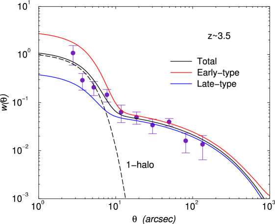
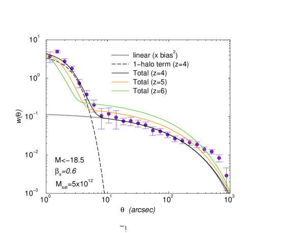
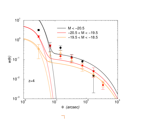
Extending to higher-redshifts, we make use of the rest B-band clustering measurements at $z\sim 3$ by Lee et al. (2005) in the GOODS survey. Due to limited number statistics, measurements only exist for the total galaxy sample though in Fig. 12 we also show the clustering of early- and late-type galaxies as well. At $z\sim 4$, the recent angular clustering measurements by Ouchi et al. (2005) in the Subaru/XMM-Newton Deep Field can also be modeled using the CLF approach. In Fig. 13 (left panel), we show the measurements with $i$-band magnitudes brighter than 27.5. This magnitude limit roughly corresponds to the rest $M_{B}<-18.5$, and this conversion is consistent with the galaxy number density expected from the rest B-band galaxy LF at a redshift of 4 (with a number density of $5\times 10^{-3}$ h${}_{70}^{3}$ Mpc^-3 from Cooray 2005b) and the suggested number density of $5.8\pm 1.4\times 10^{-3}$ h${}_{70}^{3}$ Mpc^-3 in Ouchi et al. (2005: see their Table 1) down to the same magnitude limit. To describe non-linear clustering at these redshifts, the satellite CLF must have distinctively different parameters for the slope $\beta_{s}$ and the low mass cut-off $M_{\rm sat}$ for the appearance of satellites when compared to parameters. In Figure 1, we show the expected clustering level based on best-fit parameters that we will return to below. For comparison, in the same figure, we also show expected clustering of galaxies down to the same magnitude level at redshifts 5 and 6. At large angular scales, as the redshift is increased, clustering strength is expected to increase due to redshift evolution of bias factor, which is in return associated with the decreasing number density of halos that host the galaxies with the same luminosity when compared to the number density at a lower redshift. At small scales corresponding to the 1-halo term, galaxy clustering should show a decrease in strength as the number of galaxies that appear as satellites with the same luminosity is decreasing as the redshift is increased.

In Fig. 13 (right panel), we consider clustering as a function of the galaxy luminosity at $z\sim 4$. The measurements shown here now come from Kashikawa et al. (2005) based on clustering measured with the Subaru Deep Field. To describe luminosity dependent galaxy clustering we use the same CLFs as the ones used to describe galaxy clustering at $z\sim 4$ in the right panel, but divided the absolute luminosities of galaxies following the division in Kashikawa et al. (2005) based on apparent magnitudes. While galaxy clustering in the fainter bins are adequately described, the non-linear clustering seen in the brighter bin is overestimated. This is clearly due to a wrong choice of parameters related to the satellite CLF at $z\sim 4$ for these bright galaxies. Since our models here assume the best-fit parameters with $M_{B}<-18.5$, the over prediction of non-linear clustering for galaxies with $M_{B}<-20$ clearly shows that galaxies that appear as luminous satellites are only present with a higher cut off for $M_{\rm sat}$. While the Kashikawa et al. (2005) measurements only allow one estimate of clustering in the non-linear regime, we have begun a separate analysis of luminosity dependent clustering from the same imaging data as those used in Ouchi et al. (2005). Those measurements increase the signal-to-noise of non-linear clustering estimates as a function of redshift allowing the mass scale associated with satellites, as a function of their luminosity, be established better when compared to published measurements from Kashikawa et al. (2005) shown in Figure 13 (right panel). We will present these results in an upcoming study (Cooray & Ouchi 2005).

To study the extent to which model parameters related to the CLF can be constrained, we now model fit LFs and clustering measurements by varying various parameters in our model. From these model fits, we establish likelihoods to describe the data given model parameters. In this analysis, we only make use of published variance measurements of both the LF and clustering statistics. It is likely that the measurements are affected by a covariance resulting in correlations between clustering measurements at different physical or angular scales. The presence of a substantial covariance in angular projected correlation function is well known due to non-Gaussianities and overlapping window functions (e.g., Eisenstein & Zaldarriaga 1999; Cooray & Hu 2001). While the model based on CLFs has a large number of free parameters ($\sim 20$), various experimentation with the data showed that only a handful of parameters are constrained while other parameters remain unconstrained for various reasons. Thus, we only consider a subset of parameters to model fit while other parameters are fixed based on various other arguments and observations. For example, we fix parameters of the $L_{c}(M)$ relation and do not attempt to establish them from galaxy clustering data. As discussed in Cooray & Milosavljević (2005a), such a relation is best determined with galaxy-galaxy lensing data and we have reanalyzed $r$-band galaxy-galaxy lensing data from SDSS to reestablish the $L_{c}(M)$ relation; The central galaxy mass estimates obtained agrees well with estimates in Mandelbaum et al. (2004). In the case of the central galaxy CLF we treat $\sigma_{\rm cen}$ and $M_{\rm cen-cut}$ as free parameters, while for the satellite CLF, we take $M_{\rm sat}$ and $\beta_{s}$ as free parameters, with the value of $\gamma$ fixed at $-1$ and equation 5 fixed following the description below it. For description involving galaxy types, we take $f_{\rm cen-E}$, $M_{\rm cen}$, $M_{\rm sat}$, $L_{\rm sat}$, $g_{\rm sat-E}$, and $f_{\rm sat-E}$ as free parameters.

While there are 10 free parameters, when model fitting the data we only consider a smaller subset of these parameters for different datasets due to an important reason that some statistics are more sensitive to certain parameters when compared to others. When considering the LF of the total galaxy sample, we fit parameters $\sigma_{\rm cen}$, $M_{\rm cen-cut}$, $M_{\rm sat}$, and $\beta_{s}$, though there are no useful constraints on the latter two parameters from the LF. This is clear from Fig. 2, where we show that the LF is mostly determined by statistics of central galaxies; Another way to explain this is that, at a given luminosity, the total density of galaxies is dominated by a larger fraction of central galaxies in low mass halos, which have a higher density, than satellites of the same luminosity in more massive halos.

In the case of LFs of galaxy types, with early- and late-type galaxies fitted simultaneously given that parameters describing early-type galaxies also describe late-type galaxies, we take $\sigma_{\rm cen}$, $M_{\rm cen-cut}$, $f_{\rm cen-E}$ and $M_{\rm cen}$ as free parameters. Figs. 14 and 15 right panels show constraints on two parameters from this parameter set with likelihood of other parameters marginalized over. In the case of the total correlation function, as a function of luminosity from SDSS, we fit $\sigma_{\rm cen}$, $M_{\rm cen-cut}$, $M_{\rm sat}$, and $\beta_{s}$, and show parameter constraints on the central galaxy CLF in Figure 14 to be compared with constraints for same parameters from the total galaxy LF.

We use the same set of parameters as the ones used to fit galaxy type LFs to also fit the correlation functions divided to galaxy types from SDSS. The constraints on $f_{\rm cen-E}$ and $M_{\rm cen}$ are shown in Fig. 15 can be compared with constraints for same parameters from the galaxy LF. Since parameters related to satellite CLF are better described with the correlation function, we expanded the parameter space and also fitted parameters related to satellite galaxy types. The constraints on these parameters, with ones related to central galaxies marginalized over based on LF constraints, are shown in Fig. 16. Beyond SDSS, we also consider model fits separately to the total clustering data at different redshifts separated into galaxy luminosities when available. Here, we treat $\sigma_{\rm cen}$, $M_{\rm cen-cut}$, $M_{\rm sat}$, and $\beta_{s}$ as free parameters as there is no information related to galaxy types in the high redshift data except in DEEP2, though we do not use that information explicitly since DEEP2 clustering measurements do not probe non-linear clustering in detail. Fig. 17 summarizes these results for parameters related to the satellite galaxy CLF.

As shown in Figs. 14 and 15, the total LF and LFs galaxy types in SDSS allow better estimates of parameters such as $\sigma_{\rm cen}$, the log-normal scatter in the $L_{c}(M)$ relation at a given mass, and $f_{\rm cen-E}$ the fraction of early-type galaxies that are in halo centers. From the SDSS total LF data down to $M_{r}<-17$ (from Blanton et al. 2004), $\sigma_{\rm cen}$ is constrained to be $0.17^{+0.01}_{-0.02}$ at the 68% confidence. In Cooray & Milosavljević (2005b), we found $\sigma_{\rm cen}\sim 0.22$ to describe the field-galaxy luminosity function in the K-band (Huang et al. 2003), while in Cooray (2005a), we suggested a value for the dispersion of $\sim$ 0.17 $\pm 0.1$ in the 2dFGRS $b_{J}$ band. Unfortunately, the underlying reason for a difference between the dispersion at K-band and lower wavelengths is not understood. Our estimate for $\sigma_{\rm cen}$ is in good agreement with the value of 0.168 found for the dispersion of central galaxy luminosities by Yang et al. (2003b) where these authors used a completely different parameterization for the CLF based on a priori assumed Schechter function shape. When compared with the Fig. 14 right panel clustering measurements do not allow stronger constraints to be placed on these two parameters when compared to the constraint based on the galaxy LF. This is due to the fact that the correlation function is more strongly sensitive to satellite galaxies rather then central galaxies through the non-linear 1-halo term.

While $\sigma_{\rm cen}$ is well determined, we find no evidence for a general low-mass cut-off in the central galaxy LF with a 95% confidence level on the upper limit of $M_{\rm cen-cut}<3\times 10^{10}$ M${}_{\hbox{$\odot$}}$. As discussed before this cut-off should not be interpreted as the M_min parameter in halo occupation number models of Zehavi et al. (2004). The cut-off suggested in models based on halo occupation number is present in CLFs through the $L_{c}(M)$ relation as shown for central galaxy CLFs in Fig. 5. We expect a global cut off in the LF if effects such as reionization (Benson et al. 2002; Bullock et al. 2000; Tully et al. 2002; see, review in Barkana & Loeb 2001) affect galaxy formation significantly. As discussed in Cooray & Cen (2005), the feedback effects may be more complex than considered before and could depend on the time scale of formation relative to the reionization (e.g., Tully et al. 2002) and additional heating history of IGM by supernovae from first galaxies. The galaxy group LFs, down to magnitudes below -13, show partial evidence for a cut off in the galaxy density corresponding to central galaxies at a halo mass around 10¹¹ M${}_{\hbox{$\odot$}}$ with a significant absence of dwarf galaxies. On the other hand, dwarf galaxy statistics in massive clusters, hosted in dark matter halos with masses much below the cut-off halo mass in galaxy groups, are consistent with the expectation based on the subhalo mass function. It is not clear why we do not detect an overall turn over given that such a cut-off is necessary to explain the low power-law slope of the $b_{J}$-band LF of 2dFGRS at the faint end (Cooray 2005a) and that galaxies in our sample do probe mass scales down to 10¹¹ M${}_{\hbox{$\odot$}}$. On the other hand, the phenomena leading to an absolute lower cut off the halo mass hosting galaxies may be local rather then affecting the galaxy population as a whole, though this does not explain the low-end difference between LFs of SDSS and 2dFGRS. In a future study, we plan to analyze the faint-end LF of SDSS in detail to address if there is evidence for a global cut off. We encourage extending clustering studies of galaxies to fainter magnitudes to obtain a better handle on their properties and to extend CLFs down to fainter luminosities than possible so far, though due to reasons that clustering statistics are not sensitive to central galaxies, it is unlikely such measurements alone would be helpful.

As shown in Fig. 15, the galaxy LF also provides best constraints on parameters related to galaxy types that appear in halo centers. Marginalizing over other parameters, we constrain at 68% confidence level $f_{\rm cen-E}=0.62\pm 0.19$, while the mass-scale $M_{\rm cen}$ describing the early-type fraction of central galaxies is $M_{\rm cen}=(3.1^{+8.2}_{-2.7})\times 10^{11}$ M${}_{\hbox{$\odot$}}$. As in Fig. 14, constraints from SDSS galaxy clustering statistics are lower when compared to constraints from the LF for same parameters. While parameters related to central galaxies are not well determined by clustering statistics, certain parameters related to satellite galaxies are. As shown in Fig. 16, while no useful constraint exist for $M_{\rm sat-type}$, as well as $L_{\rm sat}$ though we do not show its constraint here explicitly, $f_{\rm sat-E}=0.5\pm 0.15$ while $g_{\rm sat-E}=0.25\pm 0.15$ at the 68% confidence level from SDSS clustering data.

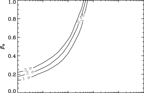
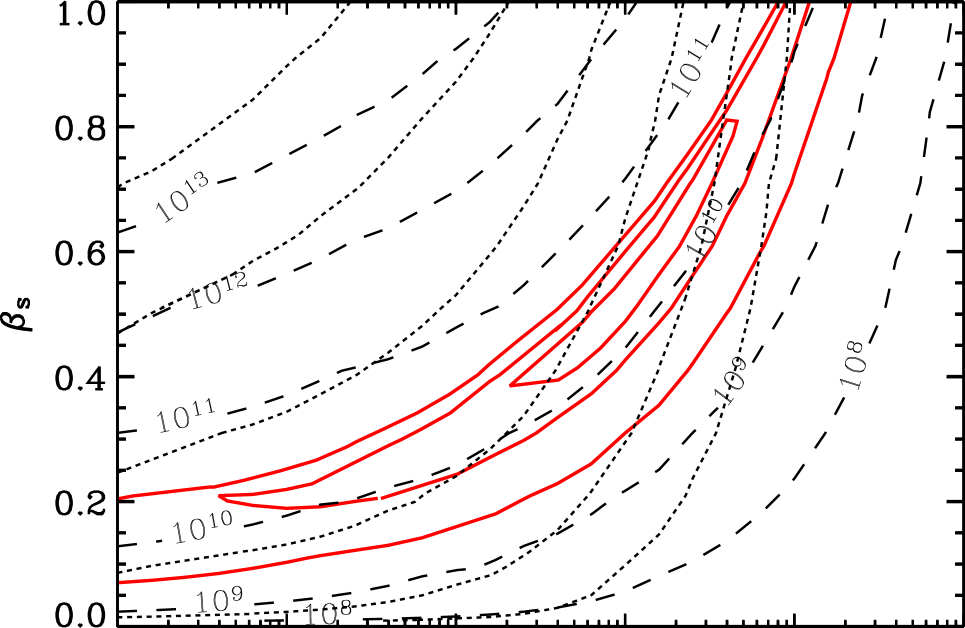
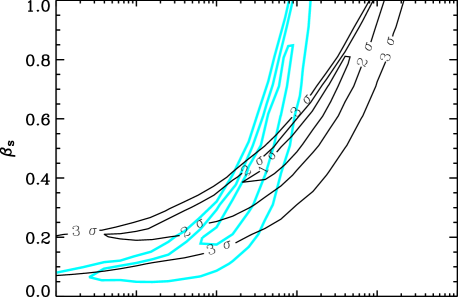
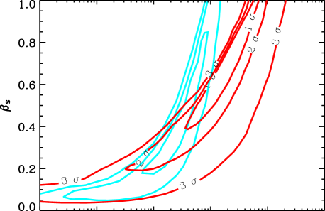
With clustering statistics, the best constraints are on parameters related to the total satellite CLF. In Fig. 17, we summarize constraints on parameters $\beta_{s}$ and $M_{\rm sat}$ as a function of redshift of the dataset. Surveys such as SDSS and COMBO-17 allow these parameters to be determined in detail. At high redshift, while Subaru data at $z\sim 4$ from Ouchi et al. (2005) allow some constraints, DEEP2 and COMBO-17 data only allow an upper limit to be placed on say $M_{\rm sat}$ at a given value of $\beta_{s}$. The contours show significant degeneracy between these two parameters even in the cases where these parameters can be separately measured from each other. For example, with SDSS, we find $M_{\rm sat}=(1.2_{-1.1}^{+2.9})\times 10^{13}$ $h^{-1}$ M${}_{\hbox{$\odot$}}$ with a power-law slope, $\beta_{s}$, of $(0.56^{+0.19}_{-0.17})$ for the total luminosity–halo mass relation, both the 68% confidence level. The mass limit can be compared to other estimates from the literature. For example, based on numerical simulations combined with semianalytic models, Zheng et al. (2004) finds that even halos of mass $10^{12.4\pm 0.1}$ M${}_{\hbox{$\odot$}}$ host satellites with $M_{r}<-19$. Note that the one-sigma lower limit of the allowed range we find from model fitting the data is $10^{12}$ M${}_{\hbox{$\odot$}}$. Our results generally applies to galaxies with $M_{r}<-17$. If we concentrate on galaxies with $M_{r}<-19$ only, we again find that the lower limit does not change significantly suggesting that the appearance of satellite galaxies with $M_{r}<-19$ in Zheng et al. (2004; see their Figure 11) in halos with mass above $10^{12.4\pm 0.1}$ M${}_{\hbox{$\odot$}}$ is not contradicted by SDSS clustering data.

At $z\sim 0.6$, COMBO-17 data allows these parameters for $M_{B}<-18$ galaxies to be constrained as $M_{\rm sat}=(3.3_{-3.0}^{+4.9})\times 10^{13}$ $h^{-1}$ M${}_{\hbox{$\odot$}}$ and $\beta_{s}=(0.62^{+0.33}_{-0.27})$ at the 68% confidence level, respectively, while at $z\sim 4$, Subaru measurements constrain these parameters for $M_{B}<-18.5$ galaxies as $(4.12_{-4.08}^{+5.90})\times 10^{12}$ $h^{-1}$ M${}_{\hbox{$\odot$}}$ and $(0.55^{+0.32}_{-0.35})$, respectively. The large range allowed for $M_{\rm sat}$, over an order of magnitude in mass at the 68% confidence level, supports the suggestion in Zehavi et al. (2004) that halo occupation models suggested there are not unique. This large range also shows that halo occupation number predicted here and the models in Zehavi et al. (2004) are likely to be consistent with each other, but given that Zehavi et al. (2004) did not present detailed fits to data, a straight forward comparison is impossible.

The degeneracy patterns in Fig. 17, however, suggest that a certain combination of $\beta_{s}$ and $M_{\rm sat}$ is better determined when compared to these two parameters separately. The degeneracy direction is such that as M_sat is decreased, $\beta_{s}$ is decreasing as well. Thus, the increase in the total number of satellite galaxies, or more appropriately in the context of CLFs, the satellite luminosity, is compensated by the decrease in $\beta_{s}$ so as to conserve the total satellite luminosity. To understand this further, we calculate the sample averaged total luminosity of satellites, over the luminosity distribution of the galaxy sample, as

$$\langle L_{\rm sat}(z)\rangle=$$ (25)

$$\frac{\int dL\int dM\Phi(L|M,z)\frac{dn(z)}{dM}\left[L_{\rm tot}(M,z)-L_{c}(M,z)\right]}{\int dL\Phi(L,z)}\,,$$

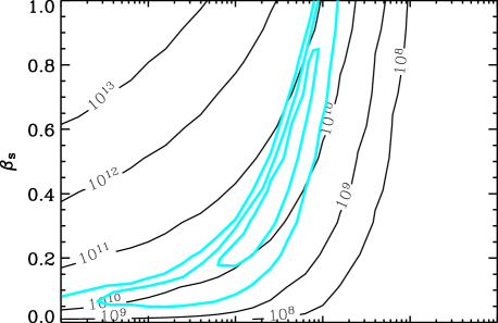
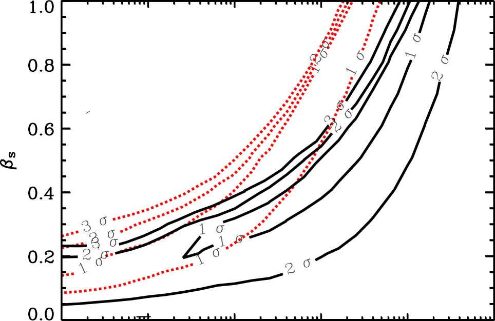
where $L_{\rm tot}(M,z)$ is given in equation (6). Since $L_{\rm tot}(M,z)$ is a function of parameters $\beta_{s}$ and $M_{\rm sat}$, we calculate $\langle L_{\rm sat}(z)\rangle$ as a function of these two parameters. In Fig. 18, we plot contours of constant $\langle L_{\rm sat}(z)\rangle$ at redshifts corresponding to SDSS and GOODS (at $z\sim 3$), and, for comparison, we also show constraints on this parameter plane from SDSS. The comparison reveals that the single parameter best constrained by the combination of $\beta_{s}$ and $M_{\rm sat}$ is $\langle L_{\rm sat}(z)\rangle$, the sample-averaged total luminosity of satellite galaxies. We find a similar behavior with other parameterization of $L_{\rm sat}(M)$ relation as well.

In Fig. 19, we plot contours of constant $\langle L_{\rm sat}(z)\rangle$ at the redshift corresponding to Subaru (at $z\sim 4$), and for comparison, in the right panel, contours of constant number density of galaxies with $M_{B}<-18.5$ at $z=4$ (in units of $10^{-3}$ h${}_{70}^{3}$ Mpc^-3) as a function of parameters related to the satellite CLF. Just as $\langle L_{\rm sat}(z)\rangle$ traces the degeneracy of the two parameters $\beta_{s}$ and $M_{\rm sat}$, the same degeneracy is traced by contours of $\bar{n}(z=4)$ as well. The range allowed by constraints on $\beta_{s}$ and $M_{\rm sat}$ is consistent with the value of $5.8\pm 1.4\times 10^{-3}$ h${}_{70}^{3}$ Mpc^-3 measured directly in the data by Ouchi et al. (2005). As shown in Fig. 19, in fact, the density is better constrained by non-linear clustering pattern when compared to a direct analysis related to the LF.

Using $\langle L_{\rm sat}(z)\rangle$ parameter instead of $\beta_{s}$ and $M_{\rm sat}$, with SDSS, we find $\langle L_{\rm sat}(z<0.1)\rangle=(2.1^{+0.8}_{-0.4})\times 10^{10}$ h^-2 L${}_{\hbox{$\odot$}}$, while with COMBO-17, $\langle L_{\rm sat}(z\sim 0.6)\rangle=(2.4^{+1.1}_{-0.6})\times 10^{10}$ h^-2 L${}_{\hbox{$\odot$}}$. Moving to higher redshifts, with DEEP2, $\langle L_{\rm sat}(z\sim 1)\rangle<3.9\times 10^{10}$ h^-2 L${}_{\hbox{$\odot$}}$, for GOODS at $z\sim 3$, $\langle L_{\rm sat}(z\sim 3)\rangle<2\times 10^{11}$ h^-2 L${}_{\hbox{$\odot$}}$, and for Subaru at $z\sim 4$, $\langle L_{\rm sat}(z\sim 4)\rangle=(4.2^{+2.3}_{-3.1})\times 10^{10}$ h^-2 L${}_{\hbox{$\odot$}}$. Based on results from SDSS and COMBO-17, if $L_{\rm sat}(z)=L_{\rm sat}(z=0)(1+z)^{\epsilon}$, then we find that $\epsilon=0.31\pm 0.52$, while between COMBO-17 and Subaru at $z\sim 4$ is $\epsilon=0.49\pm 0.74$. The difference between the two observational wavelength bands between SDSS and COMBO-17, r- and B-band respectively, and galaxy luminosities in the two samples make this comparison less useful. On the other hand, COMBO-17 sample is for galaxies with $M_{B}<-18$ while for Subaru at $z\sim 4$ is for galaxies with $M_{B}<-18.5$. While there is a small difference between the two samples, given the large redshift difference, 0.6 and 4 for COMBO-17 and Subaru data respectively, it is safe to conclude that we find no evidence for redshift evolution in the sample-averaged total luminosity of satellites.

This conclusion is in agreement with Yan et al. (2003) who compared clustering of galaxies in 2dFGRS at low redshifts and in DEEP2 and suggested no evidence for evolution between now and a redshift of unity in the total CLF as parameterized by Yang et al. (2003b). Either confirming or refuting the redshift evolution could help in understanding how satellite galaxies merge within halos to form central galaxies, whose luminosities do evolve with redshift. Given that clustering measurements by Coil et al. (2004) involved only a subset of the final DEEP2 galaxy sample, the complete analysis should improve the estimate of $\langle L_{\rm sat}\rangle$ at a redshift of 1, which when combined with SDSS and COMBO-17, should improve an estimate on the redshift evolution of $\langle L_{\rm sat}\rangle$ compared to the estimate here.

In Figure 20, we present the comparison between constraints on $\beta_{s}$ and $M_{\rm sat}$ parameters from SDSS and Subaru and COMBO-17 and Subaru respectively. While constraints on $L_{\rm sat}(z)$ show no evidence for evolution, at the 1$\sigma$ confidence level, we find that $\beta_{s}$ and $M_{\rm sat}$ parameters at $z=0.6$ and $z=4$ differ each other suggesting that these parameters in fact show some evolution. The fact that these parameters show differences (as in Figure 20), while a parameter such as $\langle L_{\rm sat}\rangle$ remain the same may, at the first instance, contradictory. The difference in parameters such as $\beta_{s}$ and $M_{\rm sat}$ between low and high redshifts comes from the difference in halo mass functions between redshifts. As the halo mass function evolves, there are no high mass halos, and satellites, if exist, should be appearing at a lower mass halo. This is the general trend we see in Figure 20. If that’s the case, one could argue that $\langle L_{\rm sat}\rangle$ should decrease as a function of increasing redshift. We do not find this behavior as halos at a high redshift gets assigned brighter central galaxies than at a low redshift due to the redshift evolution in the $L_{c}(M)$ relation. This anti-hierarchical behavior is consistent with what is generally referred to in the literature as “down-sizing” or mass-dependent luminosity evolution where brighter galaxies form first than less luminous galaxies. Since small halos are assigned brighter central galaxies at high redshift, given our description of the CLF, it is natural that such halos end up with brighter satellites as well, relative to a same mass halo at a lower redshift. Thus, while $\beta_{s}$ and $M_{\rm sat}$ change with redshift, $\langle L_{\rm sat}\rangle$ remains the same. Note that in our models of the CLF, we have not a priori assumed this behavior. In fact, CLF parameters may take any value, and we only note this behavior because of the model fitting to the data. Thus, our model fit results provide support for apparent brightening of galaxies at high redshifts both in the case of central galaxies, as discussed in Cooray 2002b, and satellites, as discussed here in terms of the clustering statistics.

In Figure 21, we show constraints on $M_{\rm sat}$ and $\beta_{s}$ as a function of the galaxy luminosity. For clarity, we only plot constraints when $-19<M_{r}<-18$ and $-22<M_{r}<-21$. These constraints reveal, though not significant, a trend in 1$\sigma$ constraint on $M_{\rm sat}$ as a function of the luminosity bin such that as galaxy luminosities are increased, $M_{\rm sat}$ is also increased. Such an increase is heavily favored in halo occupation model fits of Zehavi et al. (2004), though, we find that large uncertainties in our model parameters related to CLFs do not allow us to establish the same dependence of $M_{\rm min}$, the minimum mass for the appearance of a central galaxy in Zehavi et al. (2004), with galaxy luminosity here for the appearance of satellites through our model parameter $M_{\rm sat}$ as a function of luminosity. As stated in Zehavi et al. (2004), the halo occupation models shown there are not unique and it could be that the largely increasing values of $M_{\rm min}$ as a function of galaxy luminosity is partly accounted through unusually large power-law slopes in the halo occupation number models suggested there. It is likely that this result can be further improved with galaxy-galaxy lensing studies, and as we discuss later, more likely with cross-clustering between faint and bright galaxies.

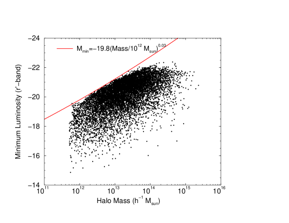
Instead of using galaxy clustering data to establish the mass scale at which satellite galaxies begins to appear, as a function of the luminosity, one can establish the same relation directly from the data if galaxy sample can be divided to a distribution of galaxy groups and clusters, with some mechanism to estimate the halo mass of that halo. Following this approach, we make use of a suggested catalog of galaxy groups in SDSS by Weinmann et al. (2005) and use the luminosity distribution to study the minimum luminosity of galaxies in these halos as a function of the halo mass. In Figure 22, we summarize our results where we consider close to $\sim 10^{4}$ groups and clusters in SDSS. The halo masses are estimated based on the total luminosity of the halo, though due to small number of galaxies when halo masses are below a few times $10^{1}2$ M${}_{\hbox{$\odot$}}$, the mass estimates may become highly uncertain. The catalog may also be affected by uncertain galaxy assignments, especially when a galaxy that is parter of a large mass halo such as cluster gets assigned systematically to a lower mass galaxy group. Ignoring these complications, which affect the low mass end, we see a trend in minimum luminosity with halo mass. This trend can be roughly described as $M_{r^{\prime}}(Min)\approx-19.8(M/10^{12}\;M_{\hbox{$\odot$}})^{0.03}$. Galaxies with luminosities greater than -21 only begin to appear in dark matter halos with mass above $10^{13}$ M${}_{\hbox{$\odot$}}$, while the mass limit for galaxies with luminosities brighter than -17 in the $r^{\prime}$-band is below 10¹² M${}_{\hbox{$\odot$}}$.

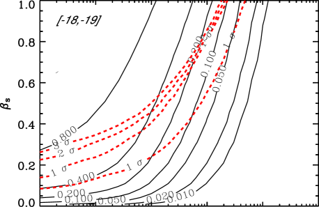
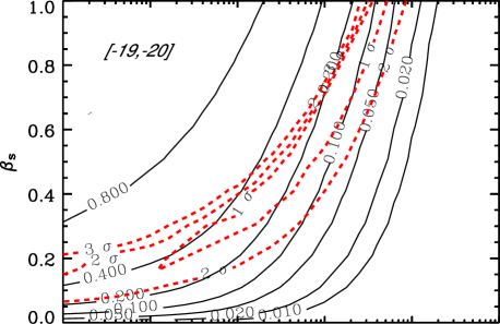
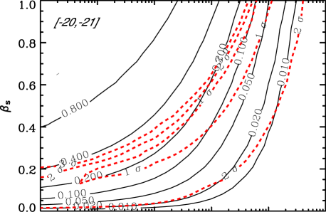
The result we derived earlier where we suggest that mass limit is $(1.2^{+2.9}_{-1.1})\times 10^{13}$ M${}_{\hbox{$\odot$}}$ is for the whole sample and is generally weighted by galaxies in magnitude bins between -19 to -21 (see, Figure 8 for example). The result based on clustering analysis is thus generally consistent with the direct estimate from the cluster catalog. In Figure 23, we plot the constraints on minimum halo mass and the power-law slope for individual bins in luminosity between -18 and -22 (dashed lines). If we make use of the general result that $M_{r^{\prime}}(Min)\approx-19.8(M/10^{12}\;M_{\hbox{$\odot$}})^{0.03}$, then we find that $\beta_{s}>0.4$ at the 3$\sigma$ confidence level. Returning to Figure 21, we then see the clear trend between minimum luminosity and the halo mass even based on galaxy clustering.

As a further application of our results, our CLFs can be easily used to estimate the average fraction of satellite galaxies in dark matter halos over a given luminosity range, $\langle f_{\rm sat}(L)\rangle$:

$$\langle f_{\rm sat}(L)\rangle=\frac{\int dM\Phi^{\rm sat}(L|M,z)\frac{dn(z)}{dM}}{\Phi(L,z)}\,.$$ (26)

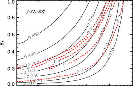
In Fig. 23, we show contours of constant $\langle f_{\rm sat}(L)\rangle$ for several luminosity bins between -18 and -22 in $M_{r}$ as appropriate for SDSS as a function of $\beta_{s}$ and M_sat. For reference, we also plot the constraint from SDSS clustering data on these two parameters as a function of the luminosity bin.

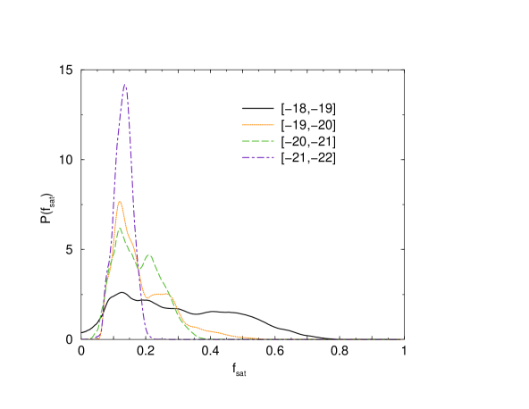
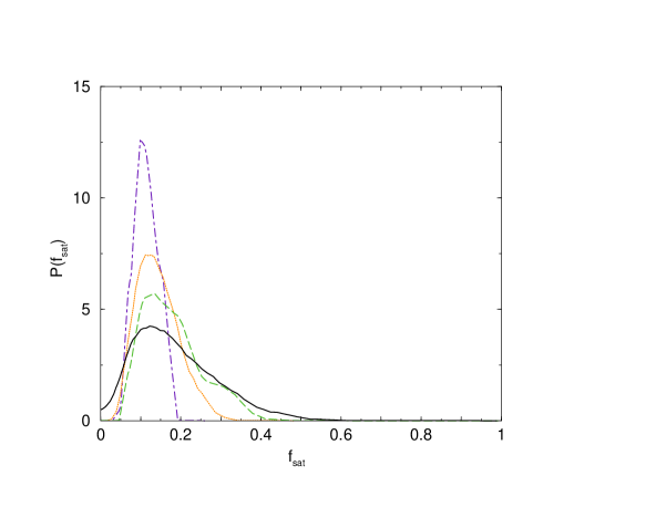
To estimate the satellite fraction as a function of the luminosity bin, instead of $M_{\rm sat}$ and $\beta_{s}$ as parameters, we determine the likelihood for the single parameter $\langle f_{\rm sat}(L)\rangle$ directly from clustering data. These results are summarized in Figure 24. The satellite fraction is in each of the bins is $0.13^{+0.03}_{-0.03}$, $0.11^{+0.05}_{-0.02}$, $0.11^{+0.12}_{-0.03}$, and $0.12^{+0.33}_{-0.05}$ for galaxies with $r^{\prime}$-band luminosities of -22 to -21, -20 to -21, -19 to -20, and -18 to -19, respectively (see, also, Figure 22). As we discussed with respect to Figure 21, there is an indication that $\beta>0.4$ to be consistent with the minimum luminosity of galaxies as a function of the halo mass. Thus, if $\beta_{s}>0.4$, the satellite fractions are $0.105^{+0.035}_{-0.025}$, $0.12^{+0.06}_{-0.05}$, $0.13^{+0.08}_{-0.05}$, and $0.13^{+0.10}_{-0.06}$, for galaxies in luminosity bins of -21 to -22, -20 to -21, -19 to -20, and -18 to -19, respectively.

Though our fractions are slightly lower, considering the errors, these fractions are fully consistent with the values suggested in Mandelbaum et al. (2004) in three luminosity bins based on an analysis of galaxy-galaxy lensing data with numerical simulations. Given that current data allow a large range of satellite fractions, for most practical purposes, one can assume that the satellite fraction is a constant with a value around 0.1 to 0.2 in luminosity bins between -18 and -21 in $M_{r}$ for general prediction calculations (e.g., Slosar et al. 2005), though when estimating cosmological parameters or other parameter constraints, it may be best to take into account suggested variations. Unlike calculations in Mandelbaum et al. (2004) or Slosar et al. (2005), in the present description of galaxy statistics with CLFs, satellite fraction is not an independent free parameter and is only determined to the extent that parameters related to the satellite CLF are known. Thus, we need not establish the satellite fraction separately.

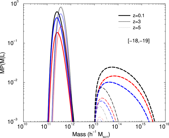
Involved with the above expression for $\langle L_{\rm sat}(z)\rangle$, in equation 4, is the probability of halo mass to a host a galaxy with luminosity $L$ at a redshift $z$ given by

$$P(M|L,z)dM=\frac{\Phi(L|M,z)}{\Phi(L,z)}\frac{dn(z)}{dM}\;dM\,.$$ (27)

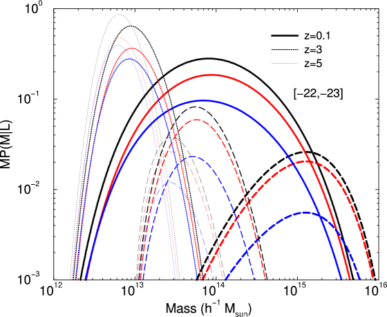
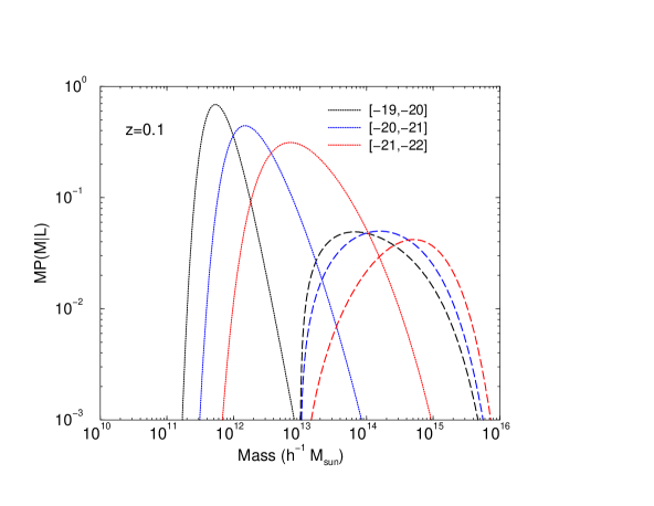
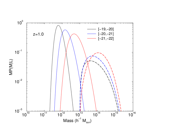
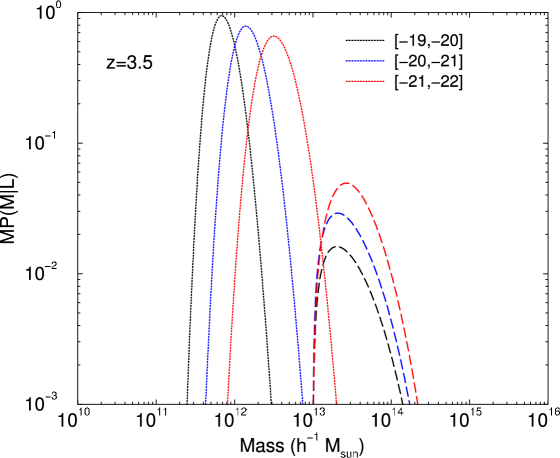
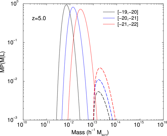
These probabilities are shown in left and right panels of Fig. 25 for a faint and a bright sample of galaxies at three different redshifts, respectively. The two panels, when combined, show the mass-dependent redshift evolution of the galaxy luminosity following Cooray (2005b). Luminous galaxies at high redshifts are found at lower mass halos than dark matter halo masses that corresponds to the same galaxy luminosity today. At the faint-end, $-18>M_{r}>-19$, regardless of the redshift, faint galaxies are essentially found in dark matter halos with a factor of 2 less range in mass, though at low redshifts, a 30% or more fraction of low-luminous galaxies could be satellites in more massive halos.

In Fig. 26, we show the same probabilities divided into three magnitude bins as a function of redshift in four panels. When $-22<M_{r}<-21$, at $z\sim 3.5$, galaxies are primarily in dark matter halos of mass $\sim 3\times 10^{12}$ M${}_{\hbox{$\odot$}}$. In comparison, such galaxies are central galaxies in groups and clusters today with masses above 10¹⁴ M${}_{\hbox{$\odot$}}$. The same probabilities have been estimated based on galaxy-galaxy weak lensing studies in SDSS by Mandelbaum et al. (2004). The mean mass estimates, at a given luminosity bin, and the dispersion of the mean mass based on probabilities shown in Fig. 26 are in agreement with estimates by Mandelbaum et al. (2004). For example, probabilities shown in Fig. 26 suggest that the mean halo mass for the bin -21 to -22 in $M_{r}$ is about $8\times 10^{12}$ h^-1 M${}_{\hbox{$\odot$}}$ which agrees with the mass estimate of $9.71\times 10^{12}$ h^-1 M${}_{\hbox{$\odot$}}$ based on NFW fits to galaxy-galaxy lensing data. Since galaxy-galaxy lensing measurements trace the galaxy–dark matter correlation function while our estimates are based solely on galaxy-galaxy clustering, these agreements suggest that to the extent probed by current data galaxy distribution traces dark matter as assumed in these halo-based models. We will, however, test this assumption in detail in an upcoming analysis.

At high redshifts, the halo masses are again consistent with various prior estimates. For example, in Conroy et al. (2004), the dark matter halo masses of $-22<M_{B}<-21$ galaxies are measured based on velocity profiles with a halo mass estimate of $5.5^{+2.5}_{-2.0}\times 10^{12}$ h^-1 M${}_{\hbox{$\odot$}}$. Our probability distribution function for halo mass in this luminosity bin and at a redshift of unity suggests a mean halo mass of $5\times 10^{12}$ h^-1 M${}_{\hbox{$\odot$}}$ in good agreement with this result. The agreement of halo masses based on galaxy LFs and prior estimates based on clustering etc at higher redshifts, in the context of LBGs, is discussed in Cooray (2005b).

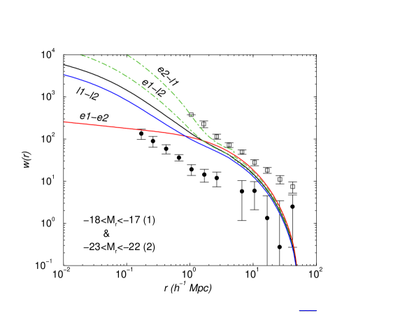
While certain parameters related to the satellite CLF are constrained well by current clustering data at low redshifts, parameters related to satellite galaxy types are not. The measurements by Zehavi et al. (2004) involve clustering of galaxies in the same luminosity bin, as well as the clustering of galaxies in the same luminosity bin and the same type (except in Figure 7, the cross-clustering between early- and late-type galaxies for $M_{r}<-21$). These measurements, while useful, do not provide all the information related to clustering for the same sample of galaxies. For example, to probe the CLF of satellites better one can consider cross-correlating galaxies that do not have a significant overlap in halo mass in terms of the central galaxy CLF. The possibility exists when considering a faint and a bright subsample of galaxies. As shown in Fig. 5, the central galaxy CLF for galaxies with $-18<M_{r}<-17$ peaks at a halo mass of few times 10¹¹ M${}_{\hbox{$\odot$}}$. The same CLF peaks at a halo mass of few times 10¹⁵ M${}_{\hbox{$\odot$}}$ when galaxies with luminosities $-23<M_{r}<-22$ are considered. While the CLF of central galaxies do not overlap, resulting in no contribution to the cross-correlation between these two samples, there is a certain overlap in the satellite CLF and to a lower extent between the central galaxy CLF of the brighter sample and the satellite CLF of the fainter sample.

The cross-correlation of galaxies between these two luminosity bins will provide an additional handle on the luminosity distribution of satellites in clusters of galaxies. In fact, one can consider cross-correlations between different luminosity bins as well as different galaxy types; For example, the cross-correlation between early type galaxies in the fainter sample and late-type galaxies in the brighter sample. We illustrate the expected cross-correlation between $-18<M_{r}<-17$ and $-23<M_{r}<-22$ galaxies in Fig. 26. For reference, in the same plot, we also show the galaxy clustering correlation function of galaxies measured by SDSS in each of the two luminosity bins. While the cross-correlation has not been measured in the data yet, we propose these additional measurements for the whole sample. Such measurements, in addition to clustering at each luminosity bin, would provide all the information related to galaxy clustering at the two-point level from any given survey. This information could in return help further constrain CLF of satellite galaxies as well as the fraction of galaxy types in the form of satellites.

While we have concentrated primarily on the use of galaxy LF and clustering measurements to constrain parameters related to central and satellite galaxy CLFs here, a primary interest of these statistical measurements is to establish global cosmological parameters. This has been achieved mostly by combining CMB data, such as from WMAP, with large-scale linear clustering with surveys such as SDSS (e.g., Tegmark et al. 2004) or with non-linear clustering part modeled based on a simple parameterization of the halo occupation number (Abazajian et al. 2005). The latter approach can be done with clustering measurements at different redshifts and the combination, as a function of redshift, would provide additional constraints on the growth evolution of density perturbations. The CLF approach suggested here may make this a possibility since CLFs provide estimates of galaxy bias, both as a function of luminosity and redshift, once the galaxy sample used for clustering measurements at various redshifts is well defined. While we have not considered cosmological parameters measurements here this is of significant interest and we hope to return to this once several high-redshift surveys provide more accurate clustering measurements for a well defined sample of galaxies.

5 Summary and Conclusions

To summarize our discussion involving model descriptions of the galaxy LF and clustering statistics with CLFs and estimates of CLF parameters directly from the data, our main results are:

(1) Instead of the halo occupation number, it may be useful to describe galaxy properties through the CLF when describing the galaxy LF and clustering statistics. As discussed in Section 2, CLFs provide a consistent way to compare, and understand, differences in measurements between different samples conditioned in terms of galaxy properties. While occupation numbers have allowed model fits to clustering statistics, their use is restricted to clustering statistics alone as LFs cannot easily be described by occupation statistics that treat all galaxies the same.

(2) We have outlined a general procedure to describe CLFs of central and satellite galaxies by improving prior descriptions of CLFs by a priori assumed Schechter function shapes (e.g., Yang et al. 2003b, 2005). The log-normal distribution for central galaxies and the power-law assumption for satellites combine to produce an overall Schechter function shape for galaxy LF (e.g., Cooray & Milosavljević 2005b), but at the same time, also explain why the cluster LF (e.g., Trentham & Tully 2002) cannot be explained with a single Schechter function.

(3) The combination of SDSS LF and clustering data at low redshifts and clustering measurements at high redshifts allow certain model parameters related to central and satellite galaxy CLFs be determined from the data. For example, the appearance of satellites with luminosities $M_{r}<-17$ at $z<0.1$, using a total luminosity–halo mass relation of the form $L_{c}(M)(M/M_{\rm sat})^{\beta}_{s}$, is constrained with SDSS to be at a halo mass of $M_{\rm sat}=(1.2_{-1.1}^{+2.9})\times 10^{13}$ $h^{-1}$ M${}_{\hbox{$\odot$}}$ with a power-law slope $\beta_{s}$ of $(0.56^{+0.19}_{-0.17})$ at the 68% confidence level. At $z\sim 0.6$, COMBO-17 data allows these parameters for galaxies with $M_{B}<-18$ to be constrained as $(3.3_{-3.0}^{+4.9})\times 10^{13}$ $h^{-1}$ M${}_{\hbox{$\odot$}}$ with a power-law slope of $(0.62^{+0.33}_{-0.27})$ at the 68% confidence level, while at higher redshifts, Subaru measurements constrain these parameters for $M_{B}<-18.5$ galaxies as $(4.12_{-4.08}^{+5.90})\times 10^{12}$ $h^{-1}$ M${}_{\hbox{$\odot$}}$ and $(0.55^{+0.32}_{-0.35})$, respectively at $z=4$. DEEP2 and GOODS measurements only allow an upper limit on the power-law slope of total luminosity at a given minimum halo mass for the appearance of satellites.

(4) The single parameter well constrained by clustering measurements is the average of total satellite galaxy luminosity corresponding to the dark matter halo distribution probed by the galaxy sample. This parameter traces the degeneracy between $M_{\rm sat}$, the minimum halo mass in which satellites appear, and $\beta_{s}$. For SDSS, $\langle L_{\rm sat}\rangle=(2.1^{+0.8}_{-0.4})\times 10^{10}$ h^-2 L${}_{\hbox{$\odot$}}$, while for GOODS at $z\sim 3$, $\langle L_{\rm sat}\rangle<2\times 10^{11}$ h^-2 L${}_{\hbox{$\odot$}}$. While current data do not suggest any redshift variation in $\langle L_{\rm sat}\rangle$, consistent with a prior suggestion (Yan et al. 2003) that CLFs do not evolve in redshift, at the 1$\sigma$ confidence level, we note that parameters related to satellite CLFs do change between $z\sim 0.6$ and $z=4$. Such a difference is expected given the redshift evolution of the halo mass function and the difference in parameters are such that the halo masses where brighter satellites appear at high redshifts host fainter satellites at low redshifts. Parameters such as the fraction of satellites at a given luminosity are not well determined by the data. Such parameters are built into the CLF description and does not need to be specified separately as in the halo models of Mandelbaum et al. (2004).

(5) In addition to constraints on central and satellite CLFs, we also determine model parameters of the analytical relations that describe the fraction of early- and late-type galaxies in dark matter halos. We use our CLFs to establish probability distribution of halo mass in which galaxies of a given luminosity could be found either at halo centers or as satellites and find good agreement with prior estimates based on an analysis of galaxy-galaxy lensing and direct mass estimates based on velocity profiles, among others.

(6) Finally, to help establish further properties of the galaxy distribution, we propose the measurement of cross-clustering between galaxies divided into different luminosity bins.

Acknowledgments: The author thanks Alison Coil, Kyoungsoo Lee, Masami Ouchi, Stefanie Phleps, and Idit Zehavi for information and electronic data files of measurements from DEEP2, GOODS, Subaru/XMM-Newton Deep Field, COMBO-17, and SDSS surveys, respectively, Uros Seljak for suggesting the inclusion of Figures 23 and 24, and an anonymous referee for suggesting the analysis based on the group catalog to determine minimum halo mass for a given luminosity (shown in Figure 22). Author also thanks members of Cosmology and Theoretical Astrophysics groups at Caltech and UC Irvine for useful discussions, and comments from the community and anonymous referees on author’s recent papers related to the CLF. This study was initiated while the author was at the Aspen Center for Physics in Summer of 2005.

References

- [Abazajian et al.¡2005¿] Abazajian, K. et al. 2005, Astrophys. J., 625, 613
- [Baldry et al.¡2004¿] Baldry, I. K., Glazebrook, K., Brinkmann, J., Ivezic, Z., Lupton, R. H., Nichol, R. C. & Sza;ary, A. S. 2004, Astrophys. J., 600, 681
- [Balogh et al.¡2004¿] Balogh, M. L., Baldry, I. K., Nichol, R., Miller, C., Bower, R., Glazebrook, K. 2004, Astrophys. J., 615, L101
- [Barkana & Loeb ¡2001¿] Barkana, R. & Loeb, A. 2001, Physics Reports, 349, 125
- [Bell et al.¡2004¿] Bell, E. F., et al. 2004, ApJ, 609, 752
- [Bell et al.¡2005¿] Bell, E. F., et al. 2005, astro-ph/0506425
- [Benson et al. ¡2000¿] Benson A. J., Cole S., Frenk C. S., Baugh C. M., Lacey C. G., 2000, MNRAS, 311, 793
- [Benson et al.¡2002¿] Benson, A. J., Lacey, C. G., Baugh, C. M., Cole, S., & Frenk, C. S. 2002, Mon. Not. R. Astron. Soc., 333, 156
- [Berlind et al.¡2004¿] Berlind, A. A., Blanton, M. R., Hogg, D. W., et al. 2004, astro-ph/0406633
- [Berlind & Weinberg ¡2002¿] Berlind A. A., Weinberg D. H., 2002, ApJ, 575, 587
- [Berlind et al.¡2003¿] Berlind, A. A., Weinberg, D. H., Benson, A. J. et al. 2003, Astrophys. J., 593, 1
- [Blanton et al.¡2003¿] Blanton, M. R. et al. 2003, Astrophys. J., 819
- [Blanton et al.¡2004¿] Blanton, M. R., et al. 2004, astro-ph/0410164
- [Bullock et al.¡2000¿] Bullock, J. S., Kravtsov, A. V., & Weinberg, D. H. 2000, Astrophys. J., 539, 517
- [Bullock et al.¡2001¿] Bullock, J. S., Kolatt, T. S., Sigad, Y. et al. 2001, Mon. Not. R. Astron. Soc., 321, 559
- [Bullock et al.¡2002¿] Bullock, J. S., Wechsler, R.S., & Somerville, R. S. 2002, Mon. Not. R. Astron. Soc., 329, 246
- [Coil et al.¡2004¿] Coil, A. L. et al. 2004, Astrophys. J., 609, 525
- [Coil et al.¡2005¿] Coil, A. L. et al. 2005, astro-ph/0507647
- [Cole & Kaiser¡1989¿] Cole, S. & Kaiser, N. 1989, Mon. Not. R. Astron. Soc., 237, 1127
- [Colless et al. ¡2001¿] Colless, M. et al. 2001, MNRAS, 328, 1039
- [Collister & Lahav ¡2005¿] Collister, A. A., Lahav O., 2005, MNRAS in press (astro-ph/0412516)
- [Conroy et al.¡2004¿] Conroy, C., et al. 2004, astro-ph/0409305
- [Cooray & Hu ¡2001¿] Cooray A., Hu W., 2001, ApJ, 554, 56
- [Cooray ¡2002¿] Cooray A. 2002, Astrophys. J., 576, L105
- [Cooray & Sheth¡2002¿] Cooray, A., & Sheth, R. 2002, Phys. Rep., 372, 1 (astro-ph/0206508)
- [Cooray & Milosavljević¡2005a¿] Cooray, A., & Milosavljević, M. 2005a, ApJ, 627, L85
- [Cooray & Milosavljević¡2005b¿] Cooray, A., & Milosavljević, M. 2005b, ApJ, 627, L89
- [Cooray ¡2005¿] Cooray, A. 2005a, Mon. Not. R. Astron. Soc., in press (astro-ph/0505421)
- [Cooray ¡2005¿] Cooray, A. 2005b, Mon. Not. R. Astron. Soc.in press (astro-ph/0506087)
- [Cooray & Cen¡2005¿] Cooray, A., & Cen, R., 2005, ApJ submitted (astro-ph/0506423)
- [Croton et al.¡2004¿] Croton, D. J. et al. 2004 Mon. Not. R. Astron. Soc.in press (astro-ph/0407537)
- [Davis et al.¡2003¿] Davis, M. et al. 2003, SPIE, 4834, 161
- [De Lucia et al.¡2004¿] De Lucia, G., Kauffmann, G., Springel, V., White, S. D. M., Lanzoni, B., Stoehr, F., Tormen, G., & Yoshida, N. 2004, Mon. Not. R. Astron. Soc., 348, 333
- [Driver & De Propis¡2002¿] Driver, S., De Propis, R. 2002, astro-ph/0212520
- [Eisenstein & Zaldarriaga¡1999¿] Eisenstein, D., Zaldarriaga, M., 1999, preprint, astro-ph/9912149
- [Efstathiou et al.¡1988¿] Efstathiou, G., Frenk, C. S., White, S. D. M. & Davis, M. 1988, Mon. Not. R. Astron. Soc., 235, 715
- [Faber et al.¡2005¿] Faber, S. M. et al. 2005, ApJ submitted, astro-ph/0506044
- [Gabasch et al.¡2004¿] Gabasch, A. et al. 2004, A&A, 421, 41
- [Giallongo et al.¡2005¿] Giallongo, E., Salimbeni, S., Menci, N. et al. 2005, Astrophys. J., 622, 116
- [Guzik & Seljak¡2002¿] Guzik, J. & Seljak, U. 2002, MNRAS, 335, 311
- [Huang et al.¡2003¿] Huang, J.-S., Glazebrook, K., Cowie, L. L, & Tinney, C. 2003, Astrophys. J., 584, 203
- [Jenkins et al.¡2001¿] Jenkins, A., Frenk, C. S., White, S. D. M., Colberg, J. M., Cole, S., Evrard, A. E., Couchman, H. M. P., & Yoshida, N. 2001, Mon. Not. R. Astron. Soc., 321, 372
- [Kashikawa et al.¡2005¿] Kashikawa, N., Yoshida, M., Shimasaku, K. et al. 2005, ApJ submitted, astro-ph/0509564
- [Kauffmann et al. ¡1999¿] Kauffmann G., Colberg J. M., Diaferio A., White S. D. M., 1999, MNRAS, 303, 188
- [Kravtsov et al.¡2004¿] Kravtsov, A. V., Berlind, A. A., Wechsler, R. H., Klypin, A. A., Gottlöber, S., Allgood, B., & Primack, J. R. 2004, Astrophys. J., 609, 35
- [Lee et al.¡2005¿] Lee, K. et al. 2005, astro-ph/0508090
- [Lin & Mohr¡2004¿] Lin, Y., & Mohr, J. J. 2004, Astrophys. J., 617, 879
- [Lin, Mohr, & Stanford¡2004¿] Lin, Y., Mohr, J. J., & Stanford, A. 2004, Astrophys. J., 610, 745
- [Mandelbaum et al.¡2004¿] Mandelbaum, R., Tasitsiomi, A., Seljak, U., Kravtsov, A. V., Wechsler, R. H. 2004, astro-ph/0410711
- [Mo et al. ¡1997¿] Mo, H. J., Jing, Y. P., White, S. D. M. 1997, Mon. Not. R. Astron. Soc., 284, 189
- [Navarro et al. ¡1997¿] Navarro, J. F., Frenk, C. S., White, S. D. M., 1997, ApJ, 490, 493
- [Norberg et al.¡2002¿] Norberg, P., et al. 2002a, Mon. Not. R. Astron. Soc., 336, 907
- [Oguri & Lee¡2004¿] Oguri, M. & Lee, J. 2004, Mon. Not. R. Astron. Soc., astro-ph/0401628
- [Ouchi et al.¡2005¿] Ouchi, M., Hamana, T., Shimasaku, K. et al. 2005, ApJ submitted, astro-ph/0508083
- [Phleps et al.¡2005¿] Phleps, S., Peacock, J. A., Meisenheimer, K., Wolf, C., 2005, astro-ph/0506320
- [Press & Schechter¡1974¿] Press, W. H., & Schechter, P. 1974, Astrophys. J., 187, 425
- [Schechter¡1976¿] Schechter, P. 1976, Astrophys. J., 203, 297
- [Scoccimarro et al. ¡2001¿] Scoccimarro R., Sheth R., Hui L., Jain B., 2001, ApJ, 546, 20
- [Seljak¡2000¿] Seljak, U. 2000, Mon. Not. R. Astron. Soc., 318, 203
- [Sheth & Tormen¡1999¿] Sheth, R. K., & Tormen, G. 1999, Mon. Not. R. Astron. Soc., 308, 191
- [Sheth, Mo, & Tormen¡2001¿] Sheth, R. K., Mo, H. J., & Tormen, G. 2001, Mon. Not. R. Astron. Soc., 323, 1
- [Sheth & Jain¡2002¿] Sheth, R. K., & Jain, B. 2002, Mon. Not. R. Astron. Soc., 345, 529
- [Slosar et al.¡2005¿] Slosar, A., Seljak, U., Tasitsiomi, A. 2005, astro-ph/0507203
- [Spergel et al.¡2003¿] Spergel, D. N., et al. 2003, Astrophys. J. Supp., 148, 175
- [Tegmark et al.¡2004¿] Tegmark, M. et al. 2004, PRD, 69, 103501
- [Trentham & Tully¡2002¿] Trentham, N., & Tully, R. B. 2002, Mon. Not. R. Astron. Soc., 335, 712
- [Tully et al.¡2002¿] Tully, R. B., Somerville, R. S., Trentham, N., Verheijen, M. A. W. 2002, Astrophys. J., 569, 573
- [Vale & Ostriker¡2004¿] Vale, A., & Ostriker, J. P. 2004, Mon. Not. R. Astron. Soc., 353, 189
- [Weinmann et al.¡2005¿] Weinmann, S. M., van den Bosch, F. C., Yang, X. & Mo, H. J. 2005, astro-ph/0509147
- [Willmer et al.¡2005¿] Willmer, C. N. A., et al. ApJ submitted, astro-ph/0506041
- [Wolf et al.¡2003¿] Wolf, C., Meisenheimer, K, Rix, H.-W., Borch, A., Dye, S. & Kleinheinrich, M. 2003, A&A, 401, 73
- [Wolf et al.¡2001¿] Wolf, C., Meisenheimer, K & Röser, H.-J. 2001, A&A, 365, 660
- [Yan et al. ¡2003¿] Yan, R., Madgwick, D. S. & White, M. 2003, Astrophys. J., 598, 848
- [Yang et al.¡2003a¿] Yang, X., Mo, H. J., Kauffmann, G., & Chu, Y. Q. 2003a, Mon. Not. R. Astron. Soc., 339, 387
- [Yang, Mo, & van den Bosch¡2003¿] Yang, X., Mo, H. J., & van den Bosch, F. C. 2003b, Mon. Not. R. Astron. Soc., 339, 1057
- [Yang et al.¡2005¿] Yang, X., Mo, H. J., Jing, Y. P., & van den Bosch, F. C. 2005, Mon. Not. R. Astron. Soc., 358, 217
- [York et al.¡2000¿] York, D. G., et al. 2000, Astron. J., 120, 1579
- [Zehavi et al.¡2004¿] Zehavi, I., et al. 2004, preprint (astro-ph/0408569)
- [Zheng et al.¡2004¿] Zheng, Z., et al. 2004, preprint (astro-ph/0408564)