Curved Space or Curved Vacuum?

Abstract

While the simple picture of a spatially flat, matter plus cosmological constant universe fits current observation of the accelerated expansion, strong consideration has also been given to models with dynamical vacuum energy. We examine the tradeoff of “curving” the vacuum but retaining spatial flatness, vs. curving space but retaining the cosmological constant. These different breakdowns in the simple picture could readily be distinguished by combined high accuracy supernovae and cosmic microwave background distance measurements. If we allow the uneasy situation of both breakdowns, the curvature can still be measured to 1%, but at the price of degrading estimation of the equation of state time variation by 60% or more, unless additional information (such as weak lensing data or a tight matter density prior) is included.

I Introduction

The acceleration of the cosmic expansion implies that in addition to the matter component of our universe there must be another energy density component (or a modification of theory that produces an effective component). The first observations of acceleration perl99 ; riess98 evoked this through plots of the amount of this dark energy density vs. matter density, based on supernova distance-redshift data. To obtain acceleration one needs both a sufficiently negative equation of state $w=p/\rho<-1/3$, and enough of this dark energy to overwhelm the deceleration due to matter. The sum of these components could add up to the critical density, and hence give spatial flatness, or not. Similarly, while the early plots considered the dark energy to be the cosmological constant, $\Lambda$ (with $w=-1$), it had long been realized that this was not the only possible accelerating component.

In looking for concordance between different types of observations, we must realize that a point in the cosmological constant density-matter density plane, $\Omega_{\Lambda}$-$\Omega_{m}$, can actually represent many models, and an apparent violation of concordance may simply indicate a breakdown in the parameter space. For example, a confidence contour disjoint from the flatness line could be a nonflat, $\Lambda$ universe, or could truly be a flat universe, but with dark energy different from the cosmological constant. That is, it could represent a breakdown of flatness of space, or of flatness of the vacuum potential energy.

In this article we analyze distance-redshift relations to distinguish these two different classes of breaking the simple cosmological model. Section II briefly discusses motivations for spatial curvature and dynamical dark energy. In §III we investigate matching the expansion rate and distances in cosmological models as a function of redshift. The qualitative difference upon allowing time variation in the dark energy equation of state is emphasized in §IV, and future observational constraints simultaneously upon spatial curvature and dark energy properties are discussed. Section V concludes.

II Spatial curvature and vacuum curvature

Even before the discovery of the accelerating expansion, models with spatial curvature or dark energy distinct from a cosmological constant were considered. Indeed, motivated by particle physics, in 1985 the cosmological relations for distance, volume, and age tests, and for some effects on primordial nucleosynthesis and the cosmic microwave background, had been developed for models with curvature and dark energy equation of state, by Wagoner (in unpublished summer school lectures, with results plotted by Linder; also see lin88a ; lin88b ). In 1986 a dark energy model with a tilted potential was invented by Linde linde86 , and that year Loh & Spillar lohspillar presented the results of observational tests, using galaxy abundances.

With the success of the inflation picture, spatial curvature came to seem repugnant. However, recent work on inflation has renewed interest in the possibility of spatial curvature (see inflacurv ; inflacurv2 and references therein). While constraints from the cosmic microwave background (CMB) and large scale structure show a consistency with flatness to 2% (68% confidence level spergel ), this assumes dark energy is the cosmological constant, and further combines several CMB and large scale structure experiments.

Flatness of the potential energy in the cosmological constant model of dark energy leads to the unhappy property that the energy density is unchanging over the history of the universe; hence the value today should be the same as in the Planck era. These eras’ energy scales are so different, however, that this requires an extraordinary coincidence in either initial conditions or the presence of us observing today.

(In fact, this phrasing of flatness vs. curvature in the potential is not wholly true. One can have a “skating” model with a flat potential but a velocity of the scalar field, $\dot{\phi}$. This will give rise to an equation of state $w^{\prime}=-3(1-w^{2})$, where $w^{\prime}=\dot{w}/H=dw/d\ln a$. The dark energy density does evolve, as $\rho_{de}\sim(1-w_{0})+(1+w_{0})a^{-6}$, but this does not avoid fine tuning problems (see also caldlin ; liddle ; joyce ). Similarly, the linear or tilted potential, while not flat, has no curvature, so we have stretched a semantic point in the title.)

The possibility of breakdown of flat space or static vacuum should therefore be considered seriously. Looking toward future precision of observational data, it is worthwhile examining in some detail the generalization to non-flat space or non-$\Lambda$ dark energy. In the next section we focus on distinguishing the two cases of breakdown of the simple model, either with both together or one at a time. §IV treats the “double trouble” case where we actually fit for spatial curvature and equation of state properties simultaneously.

III Non-flat $\Lambda$ vs. Flat non-$\Lambda$

The expansion history of the universe is basically the Hubble parameter $H(z)=\dot{a}/a$. An effective equation of state can be defined directly from this, and in particular one can consider the effective equation of state due to multiple dark energies, or to dark energy plus spatial curvature. Linder lingrav showed for an expansion history $(H/H_{0})^{2}=\Omega_{m}(1+z)^{3}+\delta H_{1}^{2}+\delta H_{2}^{2}$, where $\delta H_{1}^{2}$, $\delta H_{2}^{2}$ are two arbitrary modifications of the Friedmann equation, that

$$w_{i}\equiv-1+\frac{1}{3}\frac{d\ln\delta H_{i}^{2}}{d\ln(1+z)},$$ (1)

and moreover the effective equation of state of the non-matter part of the universe is

$$w_{\rm eff}=w_{1}\frac{\delta H_{1}^{2}}{\delta H_{1}^{2}+\delta H_{2}^{2}}+w_{2}\frac{\delta H_{2}^{2}}{\delta H_{1}^{2}+\delta H_{2}^{2}}\,.$$ (2)

That paper helped pioneer investigation of dark energy models that crossed from $w>-1$ to $w<-1$ or vice versa, the so-called phantom divide. One can readily see from Eq. (2) that the sum of a model with $w<-1$ and a model with $w>-1$ gives just such a crossing.

For the particular focus of this paper, we can consider $\delta H_{1}^{2}=\Omega_{w}e^{3\int d\ln(1+z)\,[1+w]}$, $w_{1}=w$ and $\delta H_{2}^{2}=(1-\Omega_{T})a^{-2}$, $w_{2}=-1/3$, where $\Omega_{T}$ is the dimensionless total energy density, matter plus dark energy. The second component then represents spatial curvature, $\Omega_{T}-1$, which acts like a component with $w=-1/3$ in the expansion. While Eq. (2) holds for a dark energy with time varying $w$ – the generic case – and hence we can define an effective equation of state with both arbitrary dark energy and spatial curvature, for simplicity we here show the formula when $w$ is constant:

$$w_{\rm eff}(a)=w [ \Omega_{w}a^{-3(1+w)}+(-3w)^{-1}(1-\Omega_{T})a^{-2}]$$ (3)

$$/ [\Omega_{w}a^{-3(1+w)}+(1-\Omega_{T})a^{-2}].$$

If the spatial curvature is negative, $\Omega_{T}<1$, then $w_{\rm eff}$ will lie between $w$ and $-1/3$ for all $a$ (even if $w$ is not constant). However, if the spatial curvature is positive, $\Omega_{T}>1$, and dark energy dominates curvature then $w_{\rm eff}$ will be more negative than $w$; conversely, if curvature dominates dark energy then $w_{\rm eff}$ will be more positive than $-1/3$. The transition, where $w_{\rm eff}$ goes from $-\infty$ at $z$ just less than $z_{t}$, to $+\infty$ just above, occurs at $z_{t}=-1+[(\Omega_{T}-1)/\Omega_{w}]^{1/(1+3w)}$. This behavior is illustrated in Fig. 1.

Figure 1: Combining the cosmological constant and spatial curvature, $\Omega_{T}\neq 1$, leads to an expansion history $H(z)$ of a flat, possibly phantom, dark energy model with $w_{\rm eff}(z)$. Spatial curvature can thus be mimicked by dark energy in $H(z)$, but will enter differently in distance measurements.

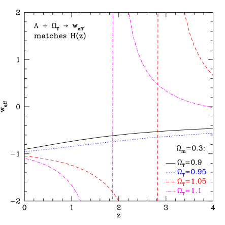
Note that we readily obtain not only models crossing $w=-1$, but can obtain a phantom equation of state, $w<-1$, using only components with $w>-1$.

Few types of observations detect the expansion history independent of the geometry of spatial curvature, i.e. the bare Hubble parameter $H(z)$, with the notable exception of the radial modes of baryon acoustic oscillation measurements linbo ; gb03 ; seoeis03 . Far more common are distance measurements, involving not only an integral of the Hubble parameter but a functional dependence on the spatial curvature. One can write the comoving distance as

$$d(z)=(1-\Omega_{T})^{-1/2}\sinh[(1-\Omega_{T})^{1/2}\int_{0}^{z}dz^{\prime}/H(z^{\prime})],$$ (4)

remembering that $\sinh$ is a complete function (i.e. the expression is valid for all $\Omega_{T}$).

Now let us consider how models with spatial curvature, but simple $\Lambda$, can mock up universes with different dark energy but retaining spatial flatness, or vice versa. To focus on the tradeoff between non-flat space and dynamic vacuum, we only consider these one at a time for the rest of this section. That is, we want to know when the distance to some redshift $z$ in a $\Lambda$ universe but with spatial curvature matches the distance to the same redshift in a spatially flat universe with constant $w$ (initially, for simplicity). So we set $d(\Omega_{m},\Omega_{T},w=-1;z)=d(\Omega_{m}^{\prime},\Omega_{T}=1,w;z)$ for some $z$. We take $\Omega_{m}^{\prime}=\Omega_{m}$ to concentrate on the effects of $\Omega_{T}$ and $w$ (also see §IV.2).

We find a complex, many-to-one, relationship between the spatial curvature in terms of $\Omega_{T}$, the dark energy equation of state $w$, and the redshift of the observations. Figure 2 shows the spatial curvature needed at each redshift in a $\Lambda$ model to match distance observations to flat universes with given values of $w$.

Figure 2: Matching distances in a non-flat, $\Lambda$ model and a flat, dark energy model indicates the interplay between the total energy density $\Omega_{T}$ needed for each redshift ($\Omega_{T}$ of course is constant in any one model) and the dark energy equation of state $w$. Both cases keep $\Omega_{m}=0.3$. This interplay varies greatly over redshift (see the text for detailed discussion), pointing out the need for distance observations over a range of redshifts to distinguish curvature from dark energy. These can be provided by, e.g., supernova measurements to $z\lesssim 2$ plus CMB measurements to $z=1089$.

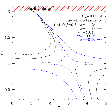
At low redshift, there is a one-to-one mapping (basically given by the deceleration parameter $q_{0}$) between $\Omega_{T}$ and $w$. In the $\Omega_{T}>1$ case, $\Omega_{\Lambda}$ has been increased so in the flat model, with $\Omega_{w}$ fixed to $1-\Omega_{m}$, $w$ must become more negative to obtain the same acceleration. However at high redshift the positive curvature becomes important, decreasing the distance to a given redshift, and so is matched by having less acceleration or a less negative $w$. Thus the matching model must cross from $w<-1$ at low redshift to $w>-1$ at high redshift. The reverse occurs for $\Omega_{T}<1$. At some point in between of course the two effects in the $\Omega_{T}\neq 1$ model cancel out and the distance is insensitive to the spatial curvature. The redshift dependence of interpreting $\Omega_{T}$ vs. $w$ in distance measurements was pointed out in lin01 , and the nulling redshift explicitly discussed in linbo5 .

In addition, at redshifts above and below the nulling redshift the matching becomes double-valued. For example a flat model with $w=-1.1$ matches the distance to $z=1.5$ of a $\Lambda$ model with either $\Omega_{T}=1.11$ or 1.88. Likewise a flat model with $w=-0.9$ matches a $\Lambda$ model with $\Omega_{T}=0.875$ or 1.895. This double valued behavior is cut off at high $\Omega_{T}$ (and low redshift) by requiring a Big Bang; larger values of $\Omega_{\Lambda}$ would cause a bounce in the past. Note that there is an attractor on the upper branch, where different values of $w$ match the same $\Omega_{T}$ as they approach the “no Big Bang” state. At low $\Omega_{T}$ the cut off is due to requiring positive $\Lambda$. At asymptotically high $z$, there is an attractor at $\Omega_{T}=1$, since in the flat model the dark energy fades away and the expansion sees a pure matter dominated state.

The implications of this distance matching are: 1) At low redshifts, $z\lesssim 1$, curvature is roughly degenerate with a shift in $w$ from $-1$. Distance observations at somewhat higher redshifts can break this. 2) Distance observations at the nulling redshift ($z=3.1$ for a fiducial flat, $\Omega_{m}=0.3$ model) are quite insensitive to curvature. This is a favored redshift range for ground based baryon acoustic oscillation measurements, meaning that such alone will not be able to provide tight constraints on spatial curvature. On the plus side, at this nulling redshift the variance of other parameters will be lessened because of zero covariance with curvature. 3) Distance measurements at very high redshift again have some sensitivity to curvature, and as this redshift increases one gets the best of points 1 and 2: the curvature influences the distance, but has reduced degeneracy with the dark energy properties.

A nice extension of lin01 quantifying the tradeoff of $\Omega_{T}$ vs. $w$ is given by Polarski & Ranquet polarski . Their Fig. 1, valid for $z=1.5$ (see also their Fig. 3 which has some $z=4$ information), clearly shows some of the degeneracies discussed. To see the progression of degeneracies and covariances with redshift, see Fig. 3 below. For illustration, this has been highly idealized, with other parameters fixed and distance measurements of 0.02%, constant in redshift. As expected, we see the degeneracy direction is the same at $z\approx 0-1$, agreeing with that of $q_{0}$; at the nulling redshift $z=3.1$ the parameters are decorrelated and $w$ is determined much better than $\Omega_{T}$; high redshift measurements are orthogonal to low redshift ones, and asymptotically the parameters decorrelate again, this time in favor of $\Omega_{T}$.

Figure 3: Covariances between total energy density $\Omega_{T}$ and constant equation of state $w$ are illustrated for idealized distance data at various redshifts (as labeled). Other parameters are fixed. The nulling redshift for curvature information is at $z\approx 3$ and high redshift distances (such as to the CMB last scattering surface) are more sensitive to curvature than to $w$.

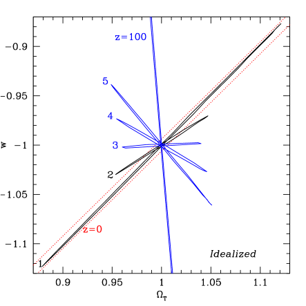
Several immediate cautions are in order. This diagram was highly idealized to bring out the degeneracy behavior. Realistic statistics, systematics (in particular gravitational lensing for high redshift measurements holzlin ), and marginalizing over the other parameters, such as the matter density and absolute source luminosity, will greatly affect the measurements and their orthogonality at different redshifts. As one example, see linsl where the orthogonality in the case of a strong lensing probe is completely undone on consideration of the realistic case. Furthermore, constant equation of state is a very specialized assumption and does not give the generic degeneracy behavior of models with time varying equation of state. We address these issues later with Fisher analysis.

Another issue is the dependence on the fiducial value of the matter density $\Omega_{m}$. For a given value of $w$ and redshift, the matching $\Omega_{T}$ changes by 1% on varying $\Omega_{m}$ between 0.2 and 0.4, except at higher redshifts or on the anomalous branch it can change by $\sim 0.2$. For a given value of $\Omega_{T}$ and redshift, the matching $w$ changes by about 1% over the same $\Omega_{m}$ range, or up to 2.5% at high $z$.

Finally, we can ask conversely what value of constant $w$ would be needed in a flat universe to match distance measurements from a nonflat, $\Lambda$ universe, as a function of redshift. This is shown in Fig. 4. Note that this is not an evolving $w(z)$ but rather a different constant $w$ to match the distance to each separate redshift. It merely provides a measure of how discrepant a single constant $w$ would be, just as in Fig. 2 the spatial curvature was not evolving but we wanted to see how the derived matching $\Omega_{T}$ from each redshift would look.

Figure 4: Matching distances in a non-flat, $\Lambda$ model and a flat, dark energy model allows derivation of the constant equation of state value, $w_{\rm const}$, that fits at any one redshift. The variation of these values from a constant indicates how strong the degeneracy is between curvature and constant $w$. Both models keep $\Omega_{m}=0.3$.

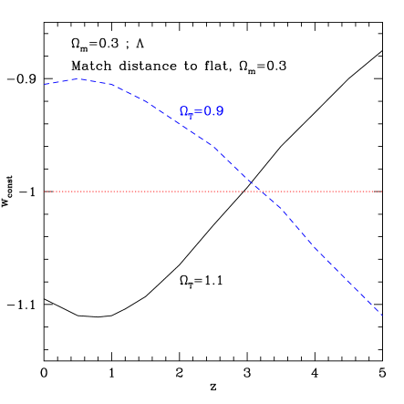
Again we see that at low redshift, $z<1$, a constant $w$ is a reasonable fit to match spatial curvature. At higher redshifts this degeneracy is broken. The nulling near $z\approx 3$ where the curves cross is clear, where very different values of spatial curvature, positive or negative, match. In the next section we extend the analysis to models with time varying equation of state, as this figure clearly indicates we must.

IV Fitting Non-flat Space and Non-static Vacuum

An orthogonal question to those we have asked so far is what if the measurements imply the simple flat, $\Lambda$ model. While simplicity would then argue for this being the favored solution, one could consider the “double trouble” case of allowing both non-flatness of space and dynamics in the vacuum to mock up the simple model. Through Fisher analysis we can see the degeneracies that would allow this and estimate the parameter constraints in a fit simultaneously accounting for $\Omega_{T}$ and $w$.

IV.1 Fitting $w_{\rm const}$ and $\Omega_{T}$

From the Fisher sensitivities of the parameters, $\partial d/\partial{\rm par}$, we can derive trade-off rules for one parameter to mock up the effects of another. For a fiducial model near the flat, $\Omega_{m}=0.3$ plus $\Lambda$ model, the trade is

$$\Delta\Omega_{T} \approx \Delta w,\quad(z\ll 1)$$ (5)

$$\approx 17\Delta w,\quad(z=3)$$ (6)

$$\approx -0.06\Delta w,\quad(z\approx z_{lss}),$$ (7)

where $z_{lss}=1089$ is the redshift of the CMB last scattering surface. These relations exhibit the sign change from low to high redshift and change in sensitivity discussed earlier. CMB results are seen to be more sensitive to spatial curvature than to the value of $w$, as is well known (e.g. hu ).

One also needs to take account of the covariances among the entire parameter set. For supernova (SN) distance measurements one has a parameter set of $\{{\cal M},\Omega_{m},\Omega_{T},w\}$, where ${\cal M}$ is a nuisance parameter combining the supernova absolute luminosity and the Hubble constant. Relaxing spatial flatness has a significant effect on parameter estimation. Even with constant $w$, data strongly constraining ${\cal M}$ (e.g. low redshift SN such as from the Nearby Supernova Factory snf ) and a tight prior on $\Omega_{m}$ (of order 0.01) are required for reasonable estimations. With both of these, and distance data from $z=0-1.7$ of the quality expected from SNAP snap , the marginalized errors are $\sigma(\Omega_{T})=0.19$ and $\sigma(w_{\rm const})=0.20$. Contrast this with the constraints $\sigma(\Omega_{T})=0.065$ when we fix $w=-1$ or $\sigma(w_{\rm const})=0.065$ when we fix $\Omega_{T}=1$ – without an $\Omega_{m}$ prior. The covariances greatly increase uncertainties over naïve expectations.

Complementarity with high redshift distances ($z\gtrsim 4$) is expected to be useful, but these distances must be known with strong statistical and systematic accuracy – a challenging task. However we found in §III that distances to $z\gg 1$ would be most useful, and the CMB data provides accurate distance measurements to $z=1089$. Adding CMB data of 0.7% precision in the reduced distance to last scattering and 0.9% on $\Omega_{m}h^{2}$ (as from the next generation Planck Surveyor experiment planck ) to SN data, and including marginalization over the reduced Hubble constant $h$, yields a simultaneous estimation with $\sigma(\Omega_{T})=0.011$ and $\sigma(w_{\rm const})=0.079$ without any additional priors. By contrast, adding even a very optimistic 1% measurement of the distance to $z=5$, which in Fig. 3 looks so orthogonal to $z\approx 1$ measurements, only gives $\sigma(\Omega_{T})=0.075$ and $\sigma(w_{\rm const})=0.19$. Thus, SN+CMB data provide good constraints in the “double trouble” scenario of breaking spatial flatness and vacuum staticness.

IV.2 Matching Time Varying Equation of State

Note that while we have marginalized over the matter density parameter, we have required that $\Omega_{m}$ in the flat model be the same as the $\Omega_{m}$ in the nonflat matching model, so far in this paper. The reason is that at high redshift matching the distances in the matter dominated era requires that $w\to 0$ to offset the difference between models with different $\Omega_{m}$ (cf. Eq. 1). However, since acceleration today implies $w<-1/3$ then matching between models with different $\Omega_{m}$ cannot be accomplished with constant $w$. Due to this, and the results of Fig. 4, we now consider models with spatial curvature and time varying equation of state.

As a first step, let us go back and look at matching the expansion history $H(z)$. As stated in the beginning of §III, Eq. (2) holds for time varying $w$ and Eq. (3) can be easily generalized by changing $a^{-3(1+w)}$ to $exp\{3\int_{a}^{1}d\ln a\,[1+w(z)]\}$. Matching the expansion $H$ is not appropriate for measurements of distance, because of the extra impact of spatial curvature as seen in Eq. (4). Suppose we wanted to match the distance in a nonflat, $\Lambda$ model to that in a flat, $w(z)\neq-1$ model, at every redshift. Upon differentiating the respective distances with respect to redshift, we find the requirement

$$H(w,\Omega_{T}=1,\Omega_{m}^{\prime};z) = H(w=-1,\Omega_{T},\Omega_{m};z)$$

$$/\cosh\left(\sqrt{1-\Omega_{T}}\int_{0}^{z}dz^{\prime}/H_{\Lambda}\right).$$

Clearly, matching $H$ will not lead to matching distances, and vice versa.

In fact, in general one cannot derive a well behaved $w(z)$ that matches the behavior of a nonflat, $\Lambda$ model. Recall that Fig. 4 showed a sequence of constant $w$ models, where the distance to redshift $z$ was given in terms of $w$ constant from 0 to $z$, and not a true $w(z)$. One might think that one could form a function $w(z)$ by interpolating between the constant $w$’s but this is fruitless.

An analogy is attempting to match the position of a car on a highway at all times. Say that a car behind our car is traveling at a constant 80 kph and a car ahead of our car travels at a constant 100 kph. Our car’s behavior is not bounded between 80 and 100 kph; it can go at 120 kph, and then 50 kph, say, and its position will still remain between the other two cars. Mathematically, the mean value theorem does not guarantee that derivatives of the function are bounded within the derivatives of the bounding functions.

If one attempts to derive a function $w(z)$ by defining it in terms of the derivative of the Hubble parameter, i.e. Eq. (1) applied to Eq. (IV.2), then one runs into pathologies. This is due to the cosh factor which reduces $H_{\Lambda}$. Eventually the cosh grows large enough that the right hand side is driven below $\Omega_{m}(1+z)^{3}$, effectively requiring a negative energy density for the dark energy, and no value of $w$ can handle the crossover to negative energies. Instead, one must be content with a derived $H(z)$, given by Eq. (IV.2). For $\Omega_{T}>1$, and $\Omega_{m}^{\prime}\leq\Omega_{m}$, one can define a $w(z)$, though its behavior is somewhat baroque.

At low redshift, however, there is no problem in deriving the distance-matching $w$. To lowest order in $z$, this is given as before by matching the deceleration parameter $q_{0}$. Then

$$w_{0}=-\frac{1}{3}+\frac{1}{3}\frac{1}{1-\Omega_{m}^{\prime}}[\Omega_{m}-\Omega_{m}^{\prime}-2(\Omega_{T}-\Omega_{m})],$$ (9)

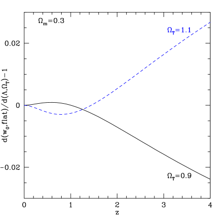
where we can now allow the matter density $\Omega_{m}^{\prime}$ of the flat, $w\neq-1$ model to differ from $\Omega_{m}$ of the nonflat, $\Lambda$ model. As discussed above, there is no point in deriving higher order terms in $w(z)$ because we know they will fail as $w$ blows up. However, we are primarily interested in the measured quantities, distances, rather than $w$ in this application. We can find the distance given by this $w_{0}$ and, although it cannot provide a perfect match to the nonflat model, ask how good an approximation it is.

Figure 5 illustrates that in fact it works well. Even though the derived $w_{0}$ is only valid for low redshift, this model approximates the nonflat, $\Lambda$ distances to better than 0.5%, or 0.01 mag, out to $z=1.8$.

Figure 5: Matching distances at several redshifts in a nonflat, $\Lambda$ model and a flat, dark energy model cannot be done with an equation of state constant with redshift. However, the fractional distance errors between these cases, shown here, are not severe out to $z\approx 2$ if the constant $w$ is chosen so as to match the deceleration parameters today (i.e. give matching distances at low redshift). For $\Omega_{T}=0.9$ (1.1), this means $w_{0}=-0.905$ (-1.095). Thus curvature could be confused with dark energy possessing constant equation of state, but not general, varying $w(z)$. Combining $z<2$ distances with the CMB last scattering distance can break the constant $w$ degeneracy.

IV.3 Fitting $w_{0}$, $w_{a}$, and $\Omega_{T}$

Finally, we consider the “triple trouble” scenario. We can examine future distance data and ask how stringent the simultaneous constraints on all the parameters are, including spatial curvature through $\Omega_{T}$ and vacuum dynamics through the dark energy equation of state characteristics $w_{0}$ and $w_{a}$, with $w(a)=w_{0}+w_{a}(1-a)$. Again, the combination of SN+CMB data is crucial to provide reasonable constraints. Furthermore, because of the extra degree of freedom in $w(a)$, without additional constraints the errors on the equation of state blow up, especially on the time variation $w_{a}$. The uncertainties in parameter estimation are $\sigma(\Omega_{T},w_{0},w_{a})=0.047$, 0.12, 1.75.

Figure 6: Allowing “triple trouble” of a non-flat, non-$\Lambda$, time varying equation of state universe strongly increases the uncertainties in the cosmological parameters, even for the combination of future supernovae and CMB data. Additional information, e.g. constraining the matter density through weak gravitational lensing data, could break the degeneracy. Combining all probes, however, removes the important element of crosschecks.

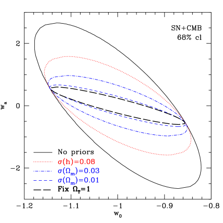
Figure 6 illustrates the severe degradation upon simultaneously estimating $\Omega_{T}$, $w_{0}$, and $w_{a}$, in contrast to assuming spatial flatness. Other parameters are marginalized over. To retain leverage on dark energy, an additional constraint is needed, for example in the form of a prior on the matter density, or other data such as weak gravitational lensing information. With a 0.03 prior on $\Omega_{m}$, the constraints improve to 0.014, 0.098, 0.64. A prior of 0.01 is required to bring the degradation in uncertainties below 10% relative to the fixed spatial flatness case, which has $\sigma(w_{0})=0.095$, $\sigma(w_{a})=0.39$. Combining with weak lensing or other large scale structure data would serve well instead, but then no room is left for crosschecks. Alternatively, the matter density can be constrained through the CMB – if the Hubble constant $h$ is accurately determined, as Hu hutucson has clearly emphasized.

V Conclusion

The exciting and fundamental property of the accelerating expansion of our universe is currently consistent with an explanation in terms of a simple cosmology flat in space and static in vacuum energy. Breakdown of one or the other of these properties can be discerned, and distinguished, with accurate distance measurements over a wide range of redshifts. Distances to the nulling redshift $z\approx 3$ are fairly insensitive to spatial curvature, and measurements at $z>3$ face severe statistical and systematic challenges – except for the CMB. For both theoretical and practical reasons, the best tools for the purpose of learning about curved space and dynamic vacuum are the combination of supernovae and cosmic microwave background distance data.

Other probes could contribute, such as baryon acoustic oscillations measurements of reduced distances and the reduced Hubble parameter, though in the $z\approx 3$ region this will mostly be in the form of breaking parameter degeneracies because of the null in sensitivity to spatial curvature. We have not considered the role of weak lensing or other large scale structure data here, though it can be quite helpful in constraining curvature bernstein ; snap ; knox , since if all probes are combined together then the important ability to crosscheck the results vanishes.

While a nonflat, $\Lambda$ universe can be distinguished from a flat, $w\neq-1$ universe, and SN+CMB data offer good constraints in the “double trouble” scenario of breaking both spatial flatness and vacuum staticness with a constant dark energy equation of state, this treatment of dark energy is highly nongeneric. Once we allow triple trouble – the possibility that $\Omega_{T}\neq 1$, $w\neq-1$, and $w\neq$ const (e.g. $w_{a}\neq 0$) – there is indeed trouble. With a realistic treatment of dark energy in terms of a time varying equation of state, removing the theoretical prejudice for spatial flatness greatly weakens our ability to probe the cosmology, even with next generation measurements.

Since in this case the dimensionless total energy density of the universe, the dark energy density, and the dark energy equation of state all evolve, theoretical prejudice is actually also motivated by multiple coincidence problems – why are we living at a time when we can see a nearly flat universe, one with roughly equal densities in dark energy and matter, and one accelerating with a behavior close to that from a cosmological constant. Perhaps as a first step we can use Occam’s razor, that entities should not be multiplied beyond necessity, backed up by inflation and the instability of $\Omega_{T}\neq 1$, to take spatial flatness as an assumption until contradicted by data. More satisfactory would be precision determination of $\Omega_{m}$ or $h$, to provide consistent constraints breaking the degeneracies.