Cosmological Parameters from the 2003 flight of BOOMERANG

Abstract

We present the cosmological parameters from the CMB intensity and polarization power spectra of the 2003 Antarctic flight of the BOOMERANG telescope. The BOOMERANG data alone constrains the parameters of the $\Lambda$CDM model remarkably well and is consistent with constraints from a multi-experiment combined CMB data set. We add LSS data from the 2dF and SDSS redshift surveys to the combined CMB data set and test several extensions to the standard model including: running of the spectral index, curvature, tensor modes, the effect of massive neutrinos, and an effective equation of state for dark energy. We also include an analysis of constraints to a model which allows a CDM isocurvature admixture.

1 Introduction

The angular power spectra of the Cosmic Microwave Background (CMB) have become invaluable observables for constraining cosmological models. The position and amplitude of the peaks and dips of the CMB spectra are sensitive to such parameters as the geometry of the Universe, the cosmological constant and the energy densities associated with baryons and cold dark matter (Bond et al., 1997). The CMB intensity spectrum has been measured with high precision on large angular scales ($\ell<600$) by the WMAP experiment (Hinshaw et al., 2003), while smaller angular scales have been probed by ground and balloon-based CMB experiments (Ruhl et al., 2003; Readhead et al., 2004a; Dickinson et al., 2004; Kuo et al., 2004; Halverson et al., 2002). These data are broadly consistent with a $\Lambda$CDM model in which the Universe is spatially flat and is composed of radiation, baryons, neutrinos and the ever mysterious duo, cold dark matter and dark energy.

One of the firm predictions of this standard model is that the CMB is intrinsically polarized. Observations of the polarization power spectra, and the correlation with the total intensity spectra can therefore be used as a powerful consistency check, as well as potentially providing additional cosmological information. On large angular scales the polarization is sensitive to the details of the reionization history and the curl component is a unique signature of tensor perturbations. On smaller angular scales the polarization spectra can verify some of the basic assumptions made in the standard model. For instance, peaks in the polarization spectra arise from the same acoustic oscillations at last scattering as those in the total intensity spectra. However, the peaks in the polarization spectra are predicted to be out of phase with the intensity peaks since the former are sourced by the velocity term of the photon-baryon fluid as opposed to its density. This effect provides the strongest constraint on the origin of the structure observed in the spectra and breaks the severe degeneracy that is introduced in models with radically broken scale invariance. These are models in which non-trivial structure may already exist in the spectrum of initial perturbations.

The recent polarization measurements of the DASI (Kovac et al., 2002), CAPMAP (Hedman et al., 2002), WMAP (Kogut et al., 2003), and CBI (Readhead et al., 2004b) experiments have confirmed that the CMB is indeed polarized, providing an independent means for testing the underlying model. Many of the standard model cosmological parameters are becoming highly constrained, especially in combination with complementary data sets (e.g. Seljak et al., 2004).

In this paper we test the standard model against the data from the 2003 long-duration balloon (LDB) flight of the BOOMERANG experiment (hereafter B03). This mission marks the instrument’s second successful trip over the Antarctic continent. The first LDB flight in December of 1998 (hereafter B98), resulted in landmark, high signal-to-noise maps of the CMB intensity anisotropy and the detection of the first few peaks of the intensity angular power spectrum (de Bernardis et al., 2000; Netterfield et al., 2002; Ruhl et al., 2003). For the 2003 flight the instrument receiver was redesigned to be polarization sensitive and the pointing system was upgraded to enable better attitude reconstruction. The B03 sky coverage is comprised of $\sim$195 hours of data over $\sim$1.8% of the sky, with an effective beam 11.5 $\pm$ 0.23 arcminutes. Instrument calibration is based on the 90 GHz and 60 GHz WMAP data and the resulting amplitude uncertainty in calibration is $\sim 2$%. A complete instrument description, and the B03 CMB and Galactic maps are given in Masi et al. (2005). The final data set from the flight is comprised of four power spectra: the intensity power spectrum, TT; the EE (curl-free) and BB (curl-like) polarization power spectra; and the TE cross-power spectrum. These spectral data are presented in Jones et al. (2005b), Montroy et al. (2005) and Piacentini et al. (2005).

This analysis examines in detail the cosmological implications of the B03 data set. We begin by outlining our required data products and methodology in Section 2. We describe in Section 3 the various data combinations that are used in this analysis. In Section 4.1 we focus on the standard $\Lambda$CDM model and, applying only weakly restrictive priors, we find that the simple parameter fits to B03 data alone are fully consistent with those derived from other existing CMB data. To this CMB data, including the B03 data, we add in recent Large Scale Structure (LSS) redshift survey data, consisting of matter power spectra from the Sloan Digital Sky Survey (SDSS) (Tegmark et al., 2003) and the 2 Degree Field Galaxy Redshift Survey (2dFGRS) (Percival et al., 2001), and determine the marginalized parameter constraints from this combined cosmological data set. In Section 4.2 we extend our analysis to include tests of several modifications of the standard model with the combined data sets.

All of the models in Section 4 share the assumption that the initial perturbations of the primordial plasma are adiabatic: in the early radiation dominated era the matter and radiation densities are all identically perturbed, giving an overall total density and hence curvature perturbation. This is not, however, the only possibility. Isocurvature modes describe the other linear combinations of matter and radiation perturbations that do not contribute a curvature perturbation initially. Models with isocurvature contributions to the perturbations give rise to distinct signatures in the total intensity and polarization spectra. The latter can be used to further constrain the possible contributions by isocurvature modes that are not ruled out by measurements of the total intensity spectrum alone. In Section 5 we explore the constraints of the B03 and other data on a model with a mixture of a dominant adiabatic mode and a sub-dominant isocurvature mode.

2 Data Products and Methodology

2.1 Summary of B03 Results

We have developed two parallel and independent pipelines that we use to reduce the B03 observations from the time-ordered data to polarization and intensity anisotropy maps, through to angular power spectra. One pipeline was developed predominantly in North America (NA pipeline) (Contaldi et al., 2005; Jones et al., 2005a) and the other predominantly in Italy (IT pipeline)(Masi et al., 2005). The purpose of constructing two separate end-to-end pipelines is to check for self-consistency at various stages during the reduction and to check for robustness in the final spectra. We have carried out an extensive comparison of the output of the NA and IT pipelines. We find excellent agreement for both the TT spectrum (Jones et al., 2005b), representing the high signal-to-noise limit, and the polarization spectra (Montroy et al., 2005; Piacentini et al., 2005) which are the most sensitive to the treatment of the experiment’s noise characteristics and systematics. B03 spectra obtained from the IT pipeline were tested with the same weak priors for the standard model case. The resulting parameter determinations are in good agreement with those reported here.

The parameter constraints presented in this analysis are based on the output of the Xfaster hybrid Monte Carlo–maximum likelihood estimator (Contaldi et al., 2005). The estimator uses a close to optimal, quadratic, Fisher matrix based estimator which is calibrated using signal only and noise only simulations of the entire data set, from time stream to final maps. It determines true polarization and total intensity angular power spectra (averaged over pre-determined $\ell$ bands) on the sky. After an arbitrary initial guess, the quadratic estimator iterates onto the maximum likelihood solution (Bond et al., 2000), $C_{B}^{\rm dat}$, with errors determined by an estimate of the Fisher matrix for all band powers self-consistently. This ensures that the variance for each band power includes contributions from all cross terms and from all spectra. This is particularly important in the case of the cross spectra, as for example with the TE sample variance which is susceptible to the TT and EE power in addition to the TE power itself.

The calculation of the full Fisher matrix also allows us to exclude band powers self consistently by cutting rows and columns from the inverse Fisher matrix. The effect of reduced sky coverage and/or pixel weighting is accounted for by computing all coupling kernels following Hivon et al. (2001) and Chon et al. (2004). The analysis typically includes a simultaneous determination of a complete set of TT, EE, BB, TE, TB, and EB band powers. The EB and TB spectra are consistent with zero (as expected) and are excluded from the parameter determination by cutting out the bands in the inverse Fisher matrix (equivalent to marginalizing over their contribution).

The spectra used in this analysis are shown in Figure 1. The data have been divided into bands which are generally $\Delta\ell$ = 50 wide for TT and $\Delta\ell$ = 100 wide for the three remaining spectra. The multipole ranges for the B03 spectra which are used in this analysis are presented in Table 1. All band-to-band correlations are included in the Fisher information matrix and are at most $\sim$20%. The band spacing was chosen in part to ensure that these correlations were not large.

Table 1: B03 bandpowers. The lowest bandpowers of the TT spectrum ($\ell<375$) are excluded when combining the B03 data with the WMAP results since the two spectra are signal dominated and therefore correlated.

B03 Spectrum	Multipole Range	Number of Bands	Reference
TT	75 (375) $\leq\ell\leq 1400$	24 (18)	Jones et al. (2005b)
TE	$150\leq\ell\leq 950$	9	Piacentini et al. (2005)
EE & BB	$150\leq\ell\leq 1000$	7	Montroy et al. (2005)

Figure 1: The B03 bandpowers used in this analysis. We have included the total intensity TT, polarization EE and BB, and cross correlation TE spectra. The EB and TB spectra are excluded from this parameter analysis. The solid/black curve is the previous concordance model, a best fit to WMAP(first-year)+CBI+ACBAR data from http://lambda.gsfc.nasa.gov/product/map/, with ($\Omega_{b}h^{2},\Omega_{c}h^{2},n_{\rm s}(k=0.05),\exp(-2\tau),A(k=0.05),h$) = (0.0224, 0.111, 0.958, 0.802, 0.739, 0.720). The yellow/dotted curve is the CMBall (Table 3)+B03 maximum likelihood $\Lambda$CDM model from this analysis with (slightly different parameterization–see text), ($\Omega_{b}h^{2},\Omega_{c}h^{2},n_{\rm s}(k=0.05),\tau,\ln(10^{10}A_{\rm s}(k=0.05)),\theta$) = (0.0228, 0.108, 0.959, 0.138, 3.12, 1.04).

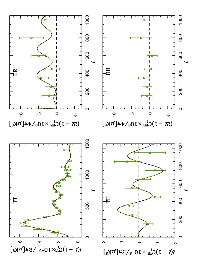
The Xfaster code also calculates the required band window functions, $W_{\ell}^{B}$, which are used to convert the model power spectra, $C^{\rm mod}_{\ell}$, into theoretical bandpowers via

$$\langle C^{\rm mod}_{B}\rangle=\frac{{\cal I}[W^{B}_{\ell}{\cal C}^{\rm mod}_{\ell}]}{{\cal I}[W^{B}_{\ell}]}$$ (1)

Here ${\cal C}^{\rm mod}_{\ell}=\ell(\ell+1)C^{\rm mod}_{\ell}/2\pi$ and we have introduced the notation for the “logarithmic integral” of a spectrum (Bond et al., 2000), ${\cal I}[f_{\ell}]\equiv\sum_{\ell}\frac{\ell+\frac{1}{2}}{\ell(\ell+1)}f_{\ell}$. The above operation permits direct comparison of theory $C^{\rm mod}_{B}$ with data $C_{B}^{\rm dat}$.

A final issue is the potential bias introduced by the non-Gaussian distribution of the bandpowers in the signal dominated regime. It has been shown (Bond et al., 2000) that the variable $Z_{B}=\ln(C_{B}^{\rm dat}+C_{B}^{N})$ is more normally distributed than the bandpowers $C_{B}$. The noise offsets, $C_{B}^{N}$, are a measure of the deconvolved noise spectrum on the sky and are calculated with the same quadratic estimator using Xfaster on the average of simulated noise-only observations.

The distribution of the bandpowers tends to a Gaussian in the noise dominated regime and log-normal in the sample variance dominated regime. Both limits are significant for the TT bandpowers, hence we transform all the TT bands to offset log-normal variables and treat the likelihood function in the new variables as Gaussian for parameter estimation. For the polarization spectra EE and BB, which are noise-dominated, we use $Z_{B}=C_{B}^{\rm dat}$, with no non-Gaussian correction. For TE we also use $Z_{B}=C_{B}^{\rm dat}$ since negative values of $C_{B}^{\rm dat}$ occur. The Fisher matrix of the bandpowers is transformed as ${\widetilde{F}}_{BB^{\prime}}=Z_{B}^{\prime}F_{BB^{\prime}}Z_{B^{\prime}}^{\prime}$ with $Z_{B}^{\prime}\equiv dZ_{B}/dC_{B}^{\rm dat}=(C^{\rm dat}_{B}+C_{B}^{N})^{-1}$ if $B$ is a TT bandpower and $Z_{B}^{\prime}=1$ otherwise.

In summary the Xfaster data products include the bandpowers, Fisher matrix, window functions and noise offsets.

2.2 Parameter Estimation Methodology

The Monte Carlo Markov Chain (MCMC) sampling technique we use for parameter estimation is described in detail in Neal (1993); Christensen et al. (2001); Lewis & Bridle (2002) and implemented in the publicly available CosmoMC package. Here we give a brief summary of the relevant details. The technique uses a Bayesian approach, generating samples of the posterior probability density function (PDF) of the parameters ${\bf y}$ given the data ${\bf z}$:

$$P(\mbox{\boldmath$y$}|{\bf z})\propto P(\mbox{\boldmath$y$})P({\bf z}|\mbox{\boldmath$y$}),$$ (2)

where $P({\bf z}|\mbox{\boldmath$y$})$ is the likelihood PDF and $P(\mbox{\boldmath$y$})$ is the prior PDF of $y$. The posterior is sampled by running a number of Markov Chains. The chains are constructed via the Metropolis-Hastings (MH) algorithm whereby a candidate parameter vector, $y^{\prime}$ is determined from an arbitrary proposal density distribution $q(\mbox{\boldmath$y^{\prime}$}|\mbox{\boldmath$y_{n}$})$ where $y_{n}$ is the current state of the chain. The candidate $y^{\prime}$ is accepted with acceptance probability given by

$$\alpha(\mbox{\boldmath$y$}|\mbox{\boldmath$y_{n}$})=\mbox{min}\left\{\frac{P(\mbox{\boldmath$y^{\prime}$}|{\bf z})q(\mbox{\boldmath$y_{n}$}|\mbox{\boldmath$y^{\prime}$})}{P(\mbox{\boldmath$y_{n}$}|{\bf z})q(\mbox{\boldmath$y^{\prime}$}|\mbox{\boldmath$y_{n}$})},1\right\}.$$ (3)

At each point in the chain the acceptance probability for a candidate point is compared to a random number $u$ drawn uniformly in the 0 to 1 range. If $u\leq\alpha(\mbox{\boldmath$y^{\prime}$}|\mbox{\boldmath$y_{n}$})$ then the proposed vector is accepted and the next point in the chain is $y_{n+1}$ = $y^{\prime}$. If $u>\alpha(\mbox{\boldmath$y^{\prime}$}|\mbox{\boldmath$y_{n}$})$ then the proposed vector is rejected and $y_{n+1}$ = $y_{n}$.

For the B03 CMB data the likelihood evaluation at each point in the chain requires the calculation of

$$\chi^{2}=\sum_{BB^{\prime}}(Z_{B}^{\rm mod}(\mbox{\boldmath$y$})-Z_{B}^{\rm dat}){\widetilde{F}}_{BB^{\prime}}(Z_{B^{\prime}}^{\rm mod}(\mbox{\boldmath$y$})-Z_{B^{\prime}}^{\rm dat}).$$ (4)

The WMAP data likelihood is computed using the likelihood code supplied by the WMAP team (Verde et al., 2003; Kogut et al., 2003), but with two modifications. The first modification is a change to the TE likelihood function to account for the correlation between the intensity and TE power spectrum estimators (we neglect the small correlations between the $C_{l}$ estimators at different $l$) (Dore et al., 2004). After the chains have been run we use importance sampling (e.g. see Lewis & Bridle (2002)) to correct the WMAP likelihood on large scales using the more computationally intensive likelihood code from Slosar et al. (2004). This Slosar-Seljak modification uses a more accurate calculation of the WMAP likelihood at low multipoles ($\ell\leq 11$) and considers in more detail the errors associated with foreground removal.

The theoretical CMB spectra (as well as the matter power spectra) are computed using CAMB (Lewis et al., 2000), a fast parallel Boltzmann code based on CMBFAST (Seljak & Zaldarriaga, 1996). We calculate statistics of interest, such as the marginalized posterior distribution of individual parameters, from the MCMC samples after removing burn in. We run six chains for each combination of data and parameters that cannot be importance sampled. We marginalize numerically over each data point’s calibration and beam uncertainties at each sample in the chain. The calibration errors are assumed to be independent between data sets. We check convergence by ensuring that the standard deviation between chains of the $95\%$-percentile estimated from each chain is less than 0.2 in units of the all-chain parameter standard deviation. This should ensure that sampling errors on quoted limits are minimal.

Parameter estimates from MCMC have been shown to be in very good agreement with those derived using an adaptive ${\cal C}_{\ell}$-grid (Bond et al., 2003) that was previously applied to the B98 analysis (Ruhl et al., 2003). MCMC results for CMBall+B98 (Bond et al., 2004) are also in good agreement with those we obtain for CMBall+B03 for the baseline model defined below with the same priors applied.

3 Data Combinations

3.1 The CMB data

We consider a number of combinations of data. We break the B03 data set into one subset consisting of the TT spectrum alone (B03TT), and another subset consisting of the EE, BB and TE spectra (B03pol) alone. We also consider fits to the entire B03 data set, WMAP data alone and a combined B03 + WMAP data set. We next combine B03 with available data from a collection of CMB experiments. We outline in Table 3 the experiments and multipole ranges which make up that collection, which we call CMBall. We note that because of the overlap in $\ell$ range of the ARCHEOPS (Tristram et al., 2005) data with the WMAP data, the former cannot be included in the CBMall data set, unless a joint analysis is done. The B03 multipole range is given in Table 1. The cosmic variance of the WMAP and B03 data sets is correlated in the low multipole range (essentially over the first peak of the TT power spectrum). To account for this, we cut the lower multipoles of the B03 TT spectrum ($\ell<375$) when combining B03 data with WMAP data.

3.2 The LSS Data

For our final data combination we also include LSS observations from 2dFGRS and the SDSS. The two redshift surveys are treated in a conservative fashion. For example, although the SDSS bandpowers have been corrected for differing galaxy bias factors associated with different types of galaxies, there is still an overall galaxy bias factor, $b_{g}$, the ratio of the square root of the galaxy-galaxy power spectrum for $L_{*}$ galaxies to that of the mass density power spectrum today. Although the indications are that this is a number near unity (Percival et al., 2001; Tegmark et al., 2003), in our standard results we allow it to take on arbitrary values by marginalizing it over a very broad distribution. This means that our LSS information is only constraining models through the shape of the power spectrum, but not the overall amplitude. Constraining the overall amplitude is akin to imposing a prior on $\sigma_{8}$. To test sensitivity to this, we have adopted varied Gaussian errors on $b_{g}^{2}$ about a mean. We have taken the mean to be unity and adopted errors on $\delta b_{g}^{2}$ appropriate for $\delta b_{g}=0,0.1,0.5$ and $10$, then marginalized over $b_{g}^{2}$. A uniform prior in $b_{g}^{2}$ leads to the same results as for $\delta b_{g}=10$ . Most parameter averages we obtain are relatively insensitive to $\delta b_{g}$. We comment on its effect below: it has impact on the massive neutrino and dark energy equation of state constraints. We only use SDSS data for wavenumbers $k<0.1h{\rm Mpc}^{-1}$ to avoid nonlinear corrections and to avoid possible non-uniform $b_{g}$ complications. (See Tegmark et al. (2003) for a discussion of these and other issues.) A similar $\delta b_{g}$ marginalization strategy was used for the 2dFGRS redshift survey data.

An estimate using galaxy-galaxy lensing from SDSS (Seljak et al., 2005) is $b_{g}=0.99\pm 0.07$. (These authors also used WMAP data to obtain this value, so it is not a completely independent determination of the bias.) An estimate using the 3-point function and redshift space clustering distortions for 2dFGRS gives $b_{g}=1.04\pm 0.04$ (Verde et al., 2002). Based on these two analyses, adopting $b_{g}=1.0\pm 0.10$ to illustrate the effect of knowing the bias better, which translates into a $\sigma_{8}$ prior, seems reasonable.

For the purposes of this paper, in which our focus is on the B03 CMB data, we have limited the LSS information we include. For example, we have not incorporated the SDSS results on luminous red galaxies (Eisenstein et al., 2005). The recent final power spectrum and window functions of the 2dFGRS survey Cole et al. (2005) is not yet available.

3.3 Other Data Sets

We have applied the supernova data (SNIa) in Section 4.2.5 to the determine the dark energy equation of state. For this we use the gold set, as described in Riess et al. (2004). Also, for a few cases we include the $H_{0}$ prior value from the HST Key Project  (Freedman et al., 2001).

We do not explicitly include weak lensing results. These generally determine the parameter combination $\sigma_{8}\Omega_{m}^{0.8}$ providing additional independent constraints (Contaldi et al., 2003; Bond et al., 2005; Readhead et al., 2004b). We also do not include information on the Lyman alpha forest, even though it probes the power spectrum to smaller scales. Although adding this data does result in some more stringent constraints than those we derive here (McDonald et al., 2004), the forest information is more susceptible to scale dependent biasing effects associated with gasdynamical and radiation processes.

4 Adiabatic Models

4.1 Baseline Model

4.1.1 Parameterization and Priors

For our baseline model we consider a flat universe with photons, baryons, massless neutrinos, cold dark matter and a cosmological constant. Initial conditions will be taken to be purely adiabatic (no isocurvature modes). We assume a power law form for the power spectrum of the primordial comoving curvature perturbation, described by ${\cal P}_{\rm s}=A_{\rm s}(k/k_{\star})^{(n_{\rm s}-1)}$, where the $n_{s}$ is the scalar spectral spectral index and $A_{s}$ is the scalar amplitude (we choose a pivot point $k_{\star}=0.05\text{Mpc}^{-1}$). The physical baryon density and dark matter density are parameterized by $\Omega_{b}h^{2}$ and $\Omega_{c}h^{2}$, where $h=H_{0}/100{\rm km}$ ${\rm s}^{-1}\text{Mpc}^{-1}$ is the Hubble parameter. We use the parameter $\theta$ to characterize the positions of the peaks in the angular power spectra, defined as one hundred times the ratio of the sound horizon to the angular diameter distance at last scattering (Kosowsky et al., 2002). Finally, the parameter $\tau$ is used to describe the Thomson scattering optical depth to decoupling. Thus our baseline model is a function of 6 cosmological parameters to which we impose the following flat weak priors: $0.5\leq n_{s}\leq 1.5$; $2.7\leq\ln(10^{10}A_{s})\leq 4.0$; $0.005\leq\Omega_{b}h^{2}\leq 0.1$; $0.01\leq\Omega_{c}h^{2}\leq 0.99$; $0.5\leq\theta\leq 10.0$; and $0.01\leq\tau\leq 0.8$. Additional weak priors restrict the age of the universe to $10\text{Gyr}\leq\text{age}\leq 20\text{Gyr}$ and the expansion rate to $0.45\leq h\leq 0.9$. All priors are summarized in Table 2. Besides being generally agreed upon by cosmologists, our weak priors are consistent with those used in much of the CMB literature, e.g., Lange et al. (2001), Bond et al. (2003) and Readhead et al. (2004b). We choose not to impose the restrictive prior $\tau<0.3$ applied in Spergel et al. (2003). We note that some of our results are sensitive to our choice of prior on $H_{0}$ and we explore the effect of strengthening our $H_{0}$ prior in Sections  4.2.1 and  4.2.2.

Table 2: List of weak priors imposed on baseline parameter set. Priors are uniform in the variable shown.

Parameter	Limits	Parameter	Limits
$\Omega_{b}h^{2}$	0.005 - 0.1	$n_{\rm s}$	0.5 - 1.5
$\Omega_{c}h^{2}$	0.01 - 0.99	$\ln[10^{10}A_{\rm s}]$	2.7 - 4.0
$\theta$	0.5 - 10.0	${\rm Age(Gyr)}$	10 - 20
$\tau$	0.01 - 0.8	$H_{0}$	45 - 90

In addition to the base parameter values, the results also include marginalized constraints for several derived parameters including: $\Omega_{\Lambda}$, the relative dark energy density; the age of the Universe; $\Omega_{m}$, the relative total matter density; $\sigma_{8}$, the root mean square linear mass perturbation in $8h^{-1}$ Mpc spheres; $z_{re}$, the redshift of reionization assuming it is a sharp transition; and the Hubble constant, $H_{0}$.

4.1.2 Consistency of B03 Data Set

The resulting marginalized parameter constraints for the baseline model for each of the data combinations are given in Table 4 and presented graphically in Figure 2. In both Table 4 (and in the ones that follow) and Figure 2 we give the Bayesian 50% probability value (the median) obtained from the marginalized probability for each parameter. The quoted errors represent the 68% confidence interval obtained by integrating the marginalized distributions. In the case of upper or lower bounds, the 95% confidence limits are quoted. We note that our baseline CMBall+B03+LSS result is fairly insensitive to $\delta b_{g}$ and that we have chosen the less restrictive flat, uniform prior in $b_{g}^{2}$.

Figure 2: Median values obtained from the marginalized probability for each parameter for the baseline, standard model. The errors bars represent the 68% confidence interval. The 95% upper limit is given for the case of $\tau$ for B03 data alone. The following flat weak priors are imposed (as outlined in Table 2): $0.5\leq n_{s}\leq 1.5$; $2.7\leq\ln(10^{10}A_{s})\leq 4.0$; $0.005\leq\Omega_{b}h^{2}\leq 0.1$; $0.01\leq\Omega_{c}h^{2}\leq 0.99$; $0.5\leq\theta\leq 10.0$; and $0.01\leq\tau\leq 0.8$. Additional weak priors restrict the age of the universe to $10\text{Gyr}\leq\text{age}\leq 20\text{Gyr}$ and the expansion rate to $45\leq H_{0}\leq 90$. Our baseline CMBall+B03+LSS result is fairly insensitive to $\delta b_{g}$ and we have chosen for this case the less restrictive flat, uniform prior in $b_{g}^{2}$.

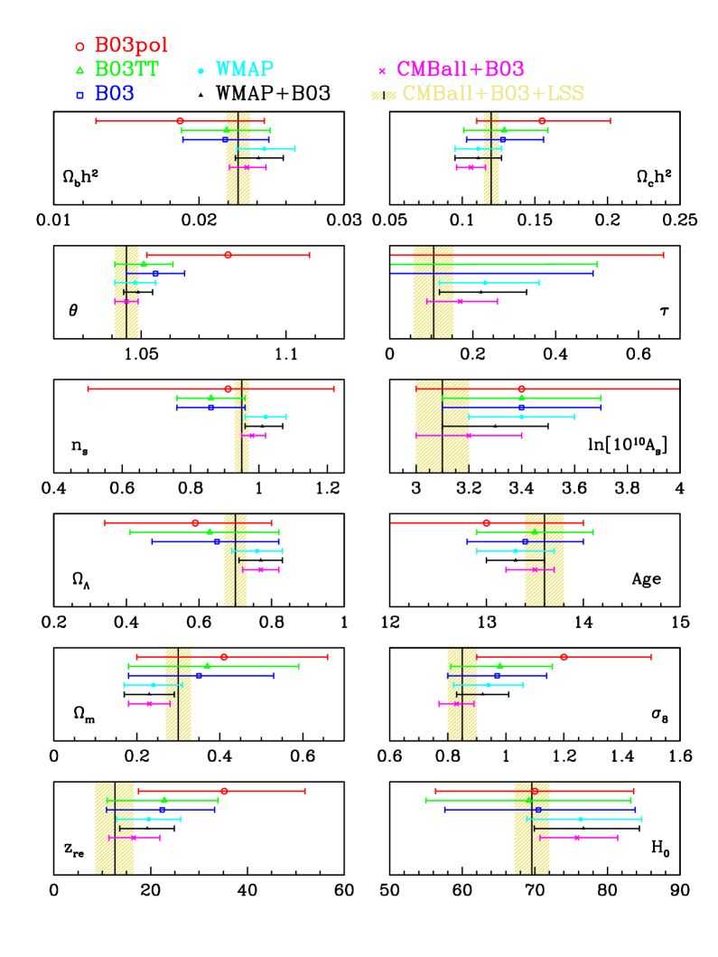
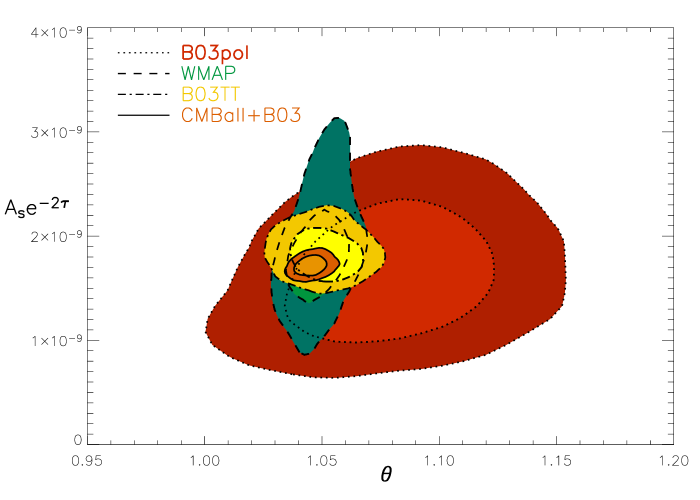
The comparison of B03pol and B03TT provides a robust internal consistency check. We note that the B03pol constraints to $\Omega_{b}h^{2}$ and $\Omega_{c}h^{2}$ are quite good with uncertainties which are only slightly larger than those of the B03TT result. However, the B03pol constraints on $n_{\rm s}$, $\tau$ and $A_{\rm s}$ are weak and results for these cases are prior driven. We present in Figure 3 a 2D likelihood plot of $\theta$ versus the combined parameter $A_{\rm s}e^{-2\tau}$. The latter determines the overall power in the observed CMB anisotropy (except at low $\ell$), and is therefore better constrained than the primordial power $A_{\rm s}$. CosmoMC uses a covariance matrix for the parameters and is therefore able to ascertain linear combination degeneracies. Although we use $\ln A_{\rm s}$ and $\tau$ as base parameters, the proposal density knows that the combination $\ln(A_{\rm s}e^{-2\tau})$ is well constrained and can explore the poorly constrained orthogonal direction efficiently. We find that the B03 data alone does particularly well at constraining $A_{\rm s}e^{-2\tau}$. The angular-diameter distance variable $\theta$ defines the shift with $\ell$ of the overall ${\cal C}_{\ell}$ pattern, in particular of the pattern of peaks and troughs. With all of the CMB data it is the best determined parameter in cosmology, $1.045\pm 0.004$; with B03pol it is an important test which demonstrates the consistency of the positions of the polarization spectra peaks and troughs relative to those forecasted from the TT data, although the errors are larger with $\theta=1.08\pm 0.03$. For the CBI TT, TE and EE data in combination with WMAP TT and TE, Readhead et al. (2004b) found $\theta=1.044\pm 0.005$. With just the CBI EE polarization data they determined $\theta=1.06\pm 0.04$, again showing the consistency we find of the data with the TT forecast of the polarization peaks and trough.

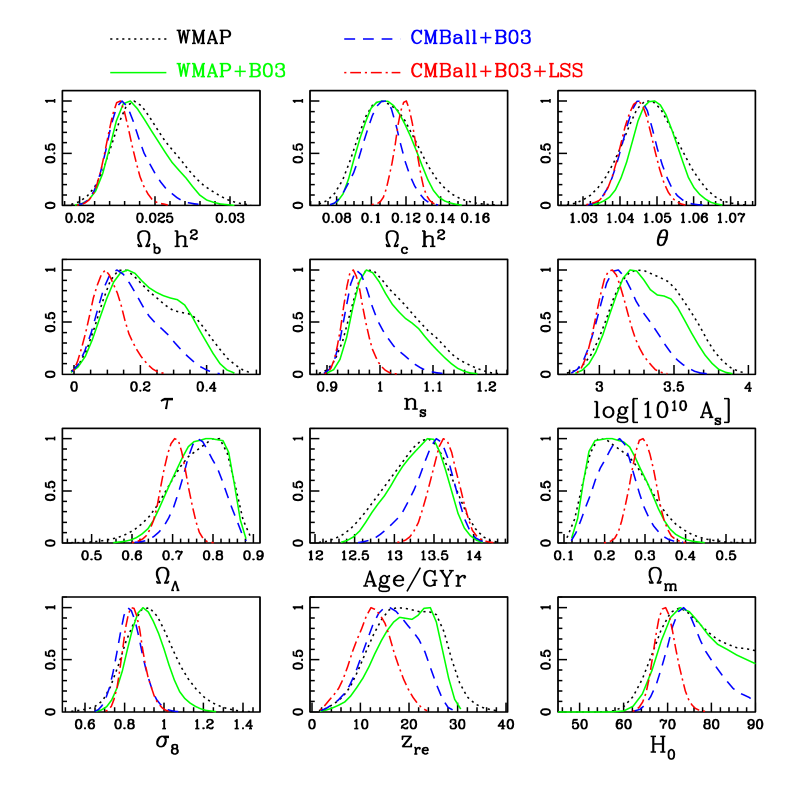
The B03 median parameter values are remarkably consistent with the parameter constraints from WMAP data alone. We note that in general the Slosar-Seljak modification to WMAP tends to broaden WMAP parameter likelihood curves and that the most significant impact on the median values is in $\tau$ ($\sim 0.3\sigma$ increase) and in $\Omega_{m}$ ($\sim 0.6\sigma$ decrease). Adding B03 to the WMAP data decreases the parameter uncertainties by an average of 16%. The most significant effect is a $\sim$33% decrease in the $\sigma_{8}$ uncertainty. Figure 4 shows the likelihood curves for the 6 base parameters and 6 derived parameters for a variety of data combinations. Overall the various data combinations are generally in good agreement at better than the $1\sigma$ level. The largest outlier is $\Omega_{c}h^{2}$ which increases by $1.5\sigma$ with the addition of the LSS data set. Also, similar to Spergel et al. (2003), we find that the addition of small scale CMB data lowers both the value for the amplitude of fluctuations at $k=0.05\text{Mpc}^{-1}$ and the value of the scalar spectral index. The effect of adding the LSS data follows this trend.

Table 3: The CMBall data set.

Experiment	Multipole Range	Reference
WMAP TT	$2\leq\ell\leq 899$	Hinshaw et al. (2003)
WMAP TE	$2\leq\ell\leq 512$	Kogut et al. (2003)
DASI TT	$380\leq\ell\leq 800$	Halverson et al. (2002)
VSA TT	$400\leq\ell\leq 1400$	Dickinson et al. (2004)
ACBAR TT	$400\leq\ell\leq 1950$	Kuo et al. (2004)
MAXIMA TT	$450\leq\ell\leq 1150$	Hanany et al. (2000)
CBI TT	$750\leq\ell\leq 1670$	Readhead et al. (2004a)

Figure 3: Constraints on $A_{\rm s}e^{-2\tau}$ versus $\theta$. Inner contours represent 68% likelihood regions and outer contours 95% likelihood regions. The peak position characterization parameter $\theta$ is best the determined parameter in cosmology, $1.045\pm 0.004$, from the CMBall+B03 data set. We find that the B03TT data does particularly well at constraining both the peak pattern and the combined $A_{\rm s}e^{-2\tau}$ amplitude parameter. The constraint from WMAP alone on $A_{\rm s}$ is better than that from B03. The agreement between the B03pol and B03TT data is consistent with the basic inflation picture.

Figure 4: Marginalized one-dimensional distributions for the baseline model parameters for the data combinations WMAP only (black/dotted), WMAP + B03 (green/solid), CMBall + B03 (blue/dashed), and CMBall + B03 + LSS (red/dash-dotted). The curves are each normalized by their peak values. All distributions are derived from chains run with the weak set of external, uniform priors shown in Table 2. The LSS data consists of the 2dFGRS and SDSS redshift surveys (with a flat $b_{g}^{2}$ prior imposed). The most significant impact of the B03 data is on ${\sigma}_{8}$. Moreover, the ${\sigma}_{8}$ constraint from CMB data alone is quite strong, with the addition of LSS data having little effect.

Table 4: Marginalized parameter constraints for the baseline, 6 parameter, $\Lambda$CDM model. Parameter uncertainties represent the 68% confidence interval obtained by integrating the marginalized distributions. 95% confidence limits are quoted for the case of upper bounds. The following flat weak priors are imposed (as outlined in Table 2): $0.5\leq n_{s}\leq 1.5$; $2.7\leq\ln(10^{10}A_{s})\leq 4.0$; $0.005\leq\Omega_{b}h^{2}\leq 0.1$; $0.01\leq\Omega_{c}h^{2}\leq 0.99$; $0.5\leq\theta\leq 10.0$; and $0.01\leq\tau\leq 0.8$. Additional weak priors restrict the age of the universe to $10\text{Gyr}\leq\text{age}\leq 20\text{Gyr}$ and the expansion rate to $45\leq H_{0}\leq 90$. The CMBall data set is as given in Table 3. The LSS data consists of the galaxy power spectra from the 2dFGRS and SDSS redshift surveys. Our baseline CMBall+B03+LSS result is fairly insensitive to $\delta b_{g}$ and we have chosen for this case the less restrictive flat, uniform prior in $b_{g}^{2}$. The constraints from the B03pol data are in good agreement with the B03TT data, although some parameters constraints for the B03pol case are prior driven, eg. $n_{\rm s},A_{\rm s}$ and $H_{0}$. B03 does not constrain $\tau$, but upper limits are given. The constraints from the various data set are consistent.

	B03pol	B03TT	B03	WMAP	WMAP	CMBall	CMBall
					+B03	+B03	+B03+LSS
$\Omega_{b}h^{2}$	$0.0187^{+0.0058}_{-0.0058}$	$0.0219^{+0.0030}_{-0.0031}$	$0.0218^{+0.0029}_{-0.0030}$	$0.0245^{+0.0021}_{-0.0019}$	$0.0241^{+0.0017}_{-0.0016}$	$0.0233^{+0.0013}_{-0.0012}$	$0.0227^{+0.0008}_{-0.0008}$
$\Omega_{c}h^{2}$	$0.155^{+0.047}_{-0.045}$	$0.129^{+0.030}_{-0.028}$	$0.128^{+0.029}_{-0.026}$	$0.111^{+0.016}_{-0.016}$	$0.109^{+0.013}_{-0.013}$	$0.106^{+0.010}_{-0.010}$	$0.120^{+0.005}_{-0.005}$
$\theta$	$1.080^{+0.028}_{-0.028}$	$1.051^{+0.010}_{-0.010}$	$1.055^{+0.010}_{-0.010}$	$1.048^{+0.007}_{-0.007}$	$1.049^{+0.005}_{-0.005}$	$1.045^{+0.004}_{-0.004}$	$1.045^{+0.004}_{-0.004}$
$\tau$	$<0.66$	$<0.50$	$<0.49$	$0.23^{+0.13}_{-0.11}$	$0.22^{+0.11}_{-0.10}$	$0.170^{+0.090}_{-0.081}$	$0.106^{+0.047}_{-0.048}$
$n_{\rm s}$	$0.91^{+0.59}_{-0.41}$	$0.86^{+0.10}_{-0.10}$	$0.86^{+0.10}_{-0.10}$	$1.02^{+0.06}_{-0.06}$	$1.01^{+0.06}_{-0.05}$	$0.98^{+0.04}_{-0.03}$	$0.95^{+0.02}_{-0.02}$
$\ln[10^{10}A_{\rm s}]$	$3.4^{+0.6}_{-0.7}$	$3.4^{+0.6}_{-0.2}$	$3.4^{+0.6}_{-0.2}$	$3.4^{+0.2}_{-0.2}$	$3.3^{+0.2}_{-0.2}$	$3.2^{+0.2}_{-0.2}$	$3.1^{+0.1}_{-0.1}$
$\Omega_{\Lambda}$	$0.59^{+0.21}_{-0.25}$	$0.63^{+0.19}_{-0.22}$	$0.65^{+0.17}_{-0.19}$	$0.76^{+0.07}_{-0.07}$	$0.77^{+0.06}_{-0.06}$	$0.77^{+0.05}_{-0.05}$	$0.70^{+0.03}_{-0.03}$
${\rm Age(Gyr)}$	$13.0^{+1.0}_{-1.0}$	$13.5^{+0.6}_{-0.6}$	$13.4^{+0.6}_{-0.5}$	$13.3^{+0.4}_{-0.4}$	$13.3^{+0.3}_{-0.3}$	$13.5^{+0.2}_{-0.3}$	$13.6^{+0.2}_{-0.2}$
$\Omega_{m}$	$0.41^{+0.25}_{-0.21}$	$0.37^{+0.22}_{-0.19}$	$0.35^{+0.19}_{-0.17}$	$0.24^{+0.07}_{-0.07}$	$0.23^{+0.06}_{-0.06}$	$0.23^{+0.05}_{-0.05}$	$0.30^{+0.03}_{-0.03}$
$\sigma_{8}$	$1.2^{+0.3}_{-0.3}$	$0.98^{+0.18}_{-0.17}$	$0.97^{+0.18}_{-0.17}$	$0.94^{+0.12}_{-0.12}$	$0.92^{+0.09}_{-0.09}$	$0.83^{+0.06}_{-0.06}$	$0.85^{+0.05}_{-0.05}$
$z_{re}$	$35.2^{+16.7}_{-17.7}$	$22.8^{+11.1}_{-11.8}$	$22.0^{+11.3}_{-11.9}$	$19.6^{+6.6}_{-6.7}$	$19.3^{+5.6}_{-5.7}$	$16.5^{+5.4}_{-5.1}$	$12.6^{+3.9}_{-4.0}$
$H_{0}$	$70.0^{+20.0}_{-25.0}$	$69.2^{+20.8}_{-24.2}$	$70.4^{+19.6}_{-25.4}$	$76.3^{+13.7}_{-4.2}$	$76.7^{+13.3}_{-3.9}$	$75.8^{+5.6}_{-5.1}$	$69.6^{+2.4}_{-2.4}$

4.2 Modified Standard Model

In this section we explore five extensions of the standard model by adding, in turn, one parameter to the baseline parameter set. In all cases we maintain the same weak priors on the base parameters as outlined in Table 2. Some of the results are sensitive to our chosen prior range for $H_{0}$. For example, in certain cases we will note the impact of strengthening our $H_{0}$ prior to the value from the HST Key Project  (Freedman et al., 2001), $h=0.72\pm 0.08$, with the errors treated as Gaussian.

4.2.1 Running Index

We modify the power law form for the power spectrum of the density perturbations to allow the spectral index, $n_{\rm s}$, to vary with scale. Following Kosowsky & Turner (1995) this variation can be parameterized by the term ${n_{\rm run}}=dn_{\rm s}/d\ln k$, such that $n_{\rm s}=n_{\rm s}(k_{\star})+{n_{\rm run}}(k_{\star})\ln(k/k_{\star})$, where again $k_{\star}=0.05\text{Mpc}^{-1}$. We restrict ${n_{\rm run}}$ to lie between -0.3 and 0.3. Results from the combined data sets, CMBall+B03 and CMBall+B03+LSS, are given in Table 5.

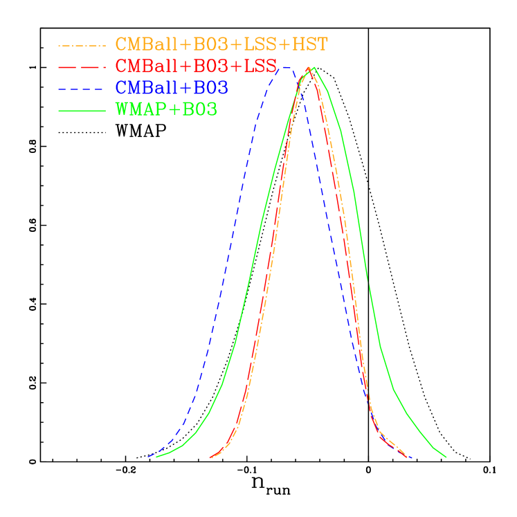
Spergel et al. (2003) report a detection of the running index of ${n_{\rm run}}=-0.031^{+0.016}_{-0.017}$ from their combined WMAPext+2dFGRS+Lyman $\alpha$ data set.  Slosar et al. (2004) present a reduction in significance of the detection of ${n_{\rm run}}$ when their full likelihood analysis and detailed foreground removal is applied to the WMAP data. We find that the Slosar-Seljak modification to WMAP decreases the significance of ${n_{\rm run}}$, but that inclusion of the data from the small scale CMB experiments has the opposite effect (as was the case found by Spergel et al. (2003)). From CMB data alone we determine a median value for ${n_{\rm run}}=-0.072\pm 0.036$. This result is somewhat sensitive to our choice of prior. Spergel et al. (2003) apply a strong $\tau<0.3$ prior which effectively reduces the median value of ${n_{\rm run}}$ for their CMB data only case. Here we apply a Gaussian HST prior on $H_{0}$ which lowers the significance of the running index to ${n_{\rm run}}=-0.065^{+0.035}_{-0.034}$ for the CMBall + B03 data set. Inclusion of the LSS data (with uniform prior in $b_{g}^{2}$) further reduces the significance and our median value from the larger combined data set is ${n_{\rm run}}=-0.051^{+0.027}_{-0.026}$. We note that the application of a Gaussian prior to $b_{g}^{2}$ has no impact on the running index parameter. Application of the HST prior on $H_{0}$ yields a final median value ${n_{\rm run}}=-0.048\pm 0.026$ for the CMBall + B03 + LSS (+HST) data set. Figure 6 shows the likelihood curves for the ${n_{\rm run}}$ parameter for various data combinations. It is interesting to compare our result with that of Seljak et al. (2004), who argue that if the state-of-the-art modeling of Lyman $\alpha$ forest measurements is dominated by statistical rather than systematic errors, then $|n_{\rm run}|<0.01$

Figure 5: Marginalized one-dimensional distributions for the ${n_{\rm run}}$ parameter for the baseline + running index model. Weak priors imposed are those outlined in Table 2. The running index parameter is restricted to lie between -0.3 and 0.3. Application of the HST prior on $H_{0}$ slightly reduces the significance of a running index.

Figure 6: Marginalized one-dimensional distributions for $\Omega_{k}$ for the baseline model which allows non-zero curvature. Weak priors imposed are those outlined in Table 2. We restrict $\Omega_{k}$ to the range -0.3 and 0.3. The relatively wide scope for positive curvature is associated with the angular-diameter-distance degeneracy which is only partly broken by the CMB data. Application of the HST prior on $H_{0}$ to the larger combined data set somewhat reduces the possibility of significant curvature.

4.2.2 Curvature

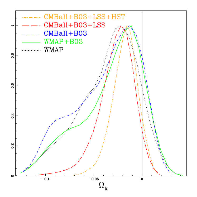
We consider a modification to the standard model which allows the possibility of non-flat geometry. We parameterize the curvature density by $\Omega_{k}$ and allow it to vary between -0.3 to 0.3. Table 5 shows the results for the CMBall+B03 and CMBall+B03+LSS data sets. The CMB data alone places a constraint on the curvature which is $\Omega_{k}=-0.037^{+0.033}_{-0.039}$. We show in Figure 6 the likelihood profiles for WMAP, WMAP+B03, CMBall+B03 and CMBall+B03+LSS. While the addition of B03 data to the WMAP data tends to lower the significance of curvature, adding more small scale CMB data increases the width of the low end tail. Addition of the LSS data, with uniform prior in $b_{g}^{2}$, yields a median value of $\Omega_{k}=-0.027\pm 0.016$. Application of the Gaussian prior in $b_{g}^{2}$ (with 10% uncertainty in $b_{g}$) has a slight effect with a resulting median value of $\Omega_{k}=-0.022\pm 0.015$. If we restrict the $H_{0}$ value by the application of a Gaussian HST prior, the curvature density determined from the CMBall + B03 data set is $\Omega_{k}=-0.015\pm 0.016$. Moreover, application of the more stringent $H_{0}$ prior reduces the median value of the curvature from the combined CMBall + B03 + LSS data set (flat $b_{g}^{2}$ prior) to $\Omega_{k}=-0.025\pm 0.017$. Our result agrees well with the constraint $\Omega_{k}=-0.010\pm 0.009$ obtained by combining CMB data with the red luminous galaxy clustering data, which has its own signature of baryon acoustic oscillations (Eisenstein et al., 2005).

4.2.3 Tensor Modes

So far we have assumed only scalar perturbations. However inflationary models can produce tensor perturbations from gravitational waves that are predicted to evolve independently of the scalar perturbations, with an uncorrelated power spectrum ${\cal P}_{\rm t}$. The amplitude of a tensor mode falls off rapidly after horizon crossing and the effect is therefore predominantly on the largest scales: tensor modes entering the horizon along the line of site to last scattering distort the photon propagation and generate an additional anisotropy pattern. We parameterize the tensor component by the ratio $A_{\rm t}/A_{\rm s}$, where $A_{\rm t}$ is the primordial power in the transverse traceless part of the metric tensor on $0.05\text{Mpc}^{-1}$ scales. We impose a very weak prior on the amplitude ratio, restricting it to lie between 0 to 20.

A tensor spectral index, defined by ${\cal P}_{\rm t}\propto k^{n_{\rm t}}$, must also be set. In inflation models it is related to the amplitude ratio by $A_{\rm t}/A_{\rm s}\approx-8n_{\rm t}/(1-n_{\rm t}/2)$, so one parameter suffices. In a nearly uniformly accelerating regime $n_{\rm t}\approx n_{\rm s}-1$ is also expected. However, although $n_{\rm s}>1$ can arise in inflation models, $n_{\rm t}>0$ is difficult to obtain. As well, for many inflation models with $n_{\rm s}-1$ just below zero, $n_{\rm t}$ comes out to be slightly closer to zero. If the acceleration changes significantly over the observably range, $n_{\rm t}$ and $n_{\rm s}$ would not be intimately tied. Rather than let $n_{t}$ float as a second added parameter, we have chosen to make ${\cal P}_{\rm t}$ flat in $k$ (and thus set $n_{\rm t}$ to zero) for the computations of the tensor-induced component of ${\cal C}_{\ell}$.

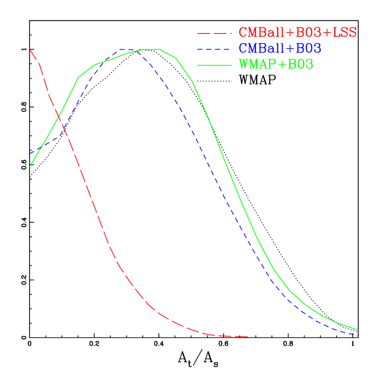
Results are presented in Table 5, and Figure 8 illustrates the likelihood curves for the amplitude ratio for a number of data combinations. The influence of the high precision of the WMAP data on the largest scales is evident. Adding the small scale CMB data only slightly reduces the limit. We determine an upper limit on the tensor ratio from CMB data (CMBall+B03 data set) alone of $A_{\rm t}/A_{\rm s}<0.71$ (95% confidence limit). The CMB data appear to select models with relatively large tensor-to-scalar ratios. However, these models which have large values for the Hubble parameter ($H_{0}\sim 85$) are allowed due to the poor constraint on $H_{0}$ when including tensor modes. In this case, the constraints on $H_{0}$ are driven mainly by our choice of weak priors and the data only provides a lower limit (see Table 5). We find with application of the HST prior (which excludes these models with large $H_{0}$ values) that the tensor limit from the CMBall+B03 data set is reduced to $A_{\rm t}/A_{\rm s}<0.635$. A similar effect is obtained with the addition of the LSS data which further reduces the limit to $A_{\rm t}/A_{\rm s}<0.36$. When we constrain $b_{g}$ in the LSS data, the limits are very similar. The application of the more restrictive prior discussed above, with only $n_{\rm s}\leq 1$ allowed to have a tensor contribution, lowers the CMBall+B03 limit to $A_{\rm t}/A_{\rm s}<0.45$ and the CMBall+B03+LSS limit to $A_{\rm t}/A_{\rm s}<0.31$. As a final case we set $n_{\rm t}=-(A_{\rm t}/A_{\rm s})/8$ and found $A_{\rm t}/A_{\rm s}<0.54$ for the CMBall+B03 data set and $A_{\rm t}/A_{\rm s}<0.30$ for the combined CMBall+B03+LSS results (again applying the $b_{g}$ constraint has little effect).

Figure 7: Marginalized one-dimensional distributions for the amplitude ratio $A_{\rm t}/A_{\rm s}$ for the baseline model modification which allows tensor modes. Weak priors imposed are those outlined in Table 2. We impose the weak prior $0<A_{\rm t}/A_{\rm s}<20$ to the tensor contribution. We find from CMB data alone (CMBall+B03) an upper limit (95% confidence) on the amplitude ratio of $A_{\rm t}/A_{\rm s}<0.71$. For these models however, $H_{0}$ is only poorly constrained (see text). Addition of the LSS data reduces this limit to $A_{\rm t}/A_{\rm s}<0.36$.

Figure 8: Marginalized one-dimensional distributions for $m_{\nu}$ for the baseline model which allows massive neutrinos (3 species of degenerate mass). Weak priors imposed are those outlined in Table 2. We parameterize the massive neutrino contribution as a fraction of the dark matter energy density, $f_{\nu}=\Omega_{\nu}h^{2}/\Omega_{DM}h^{2}$. We find from CMB data alone (CMBall+B03) an upper limit (95% confidence) on the neutrino mass of $m_{\nu}<1.0{\,\rm eV}$. Adding the LSS data reduces this limit to $m_{\nu}<0.40{\,\rm eV}$, without any $b_{g}$ constraint, and to $m_{\nu}<0.16{\,\rm eV}$, when $b_{g}=1.0\pm 0.10$ is used.

4.2.4 Massive Neutrinos

Observational evidence from solar and atmospheric neutrino experiments, such as the Sudbury Neutrino Observatory (Ahmad et al., 2002) and Super-Kamiokande (Toshito et al., 2001), suggest that neutrinos change flavour: neutrinos of different generations oscillate into each other. The implication of flavour changing is that neutrinos have mass. Given that neutrinos are the second most abundant particles in the Universe, massive neutrinos could have considerable impact on the energy density of the early Universe. We consider here the case of three neutrinos of degenerate mass, such that $\Omega_{\nu}h^{2}=3m_{\nu}/94.0{\,\rm eV}$. This assumption is well justified given the small square mass difference measured by oscillation experiments (at most $\delta m_{\nu}^{2}\sim 10^{-3}{\,\rm eV}$, Aliani et al. (2003)). We parameterize the massive neutrino contribution as a fraction of the dark matter energy density, $f_{\nu}=\Omega_{\nu}h^{2}/\Omega_{DM}h^{2}=1-\Omega_{CDM}h^{2}/\Omega_{DM}h^{2}$.

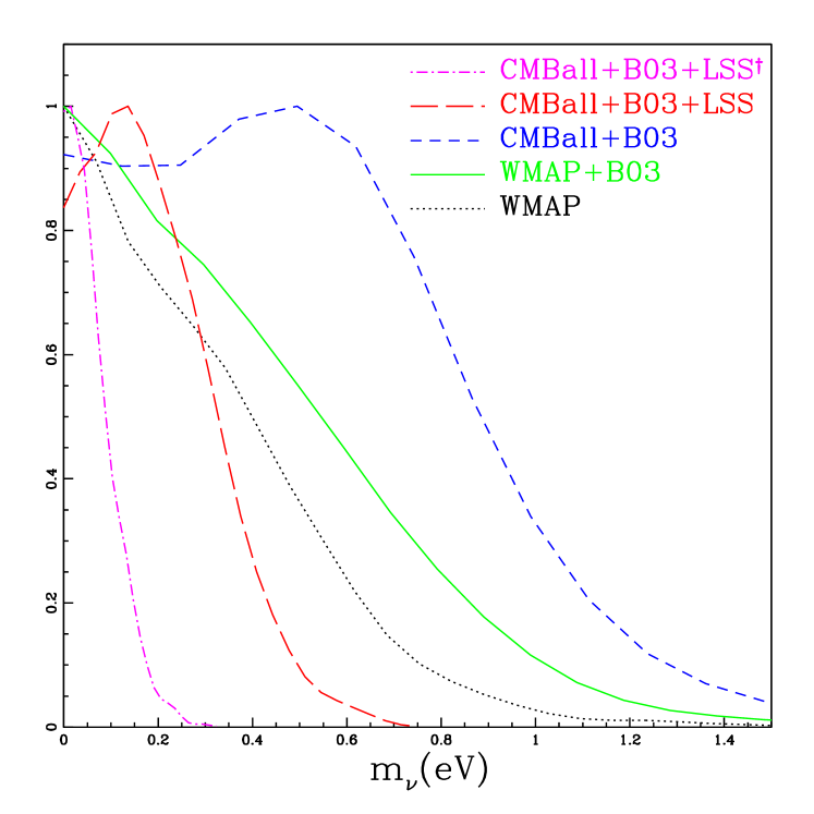
Results for the combined data sets are given in Table 5. From CMB data alone the upper limit on the neutrino fraction is $f_{\nu}<0.21$ (95% confidence limit). This translates to an upper limit on the neutrino mass of $m_{\nu}<1.0{\,\rm eV}$ or $\Omega_{\nu}h^{2}<0.033$. This limit is more stringent than the $3{\,\rm eV}$ upper limit on the electron neutrino mass determined from tritium beta decay experiments and recommended in the Review of Particle Physics (Eidelman et al., 2004). Including the LSS data (flat $b_{g}^{2}$ prior) pushes this limit down considerably to $f_{\nu}<0.093$ (95% confidence) and limits the neutrino mass to $m_{\nu}<0.40{\,\rm eV}$. This result is somewhat larger than that found in Spergel et al. (2003). We find that addition of more and more small scale CMB data drives the limit up as is evident in Figure 8. When $b_{g}=1.0\pm 0.10$ is used, the neutrino fraction upper limit is reduced to $f_{\nu}<0.041$ (95% confidence), corresponding to a neutrino mass limit of $m_{\nu}<0.16{\,\rm eV}$. This neutrino mass limit is in good agreement with the strong limit ($m_{\nu}<0.18{\,\rm eV}$) obtained by (Seljak et al., 2005), who included the bias constraint and the SDSS and WMAP data. In their analysis of $b_{g}$ they found $\sigma_{8}=0.85^{+0.07}_{-0.06}$, with $b_{g}=1.02^{+0.08}_{-0.08}$. This compares with the values we obtain: $\sigma_{8}=0.85\pm 0.04$ with $\delta b_{g}=0.10$ and $\sigma_{8}=0.74\pm 0.08$ with $\delta b_{g}=\infty$.

4.2.5 Dark Energy

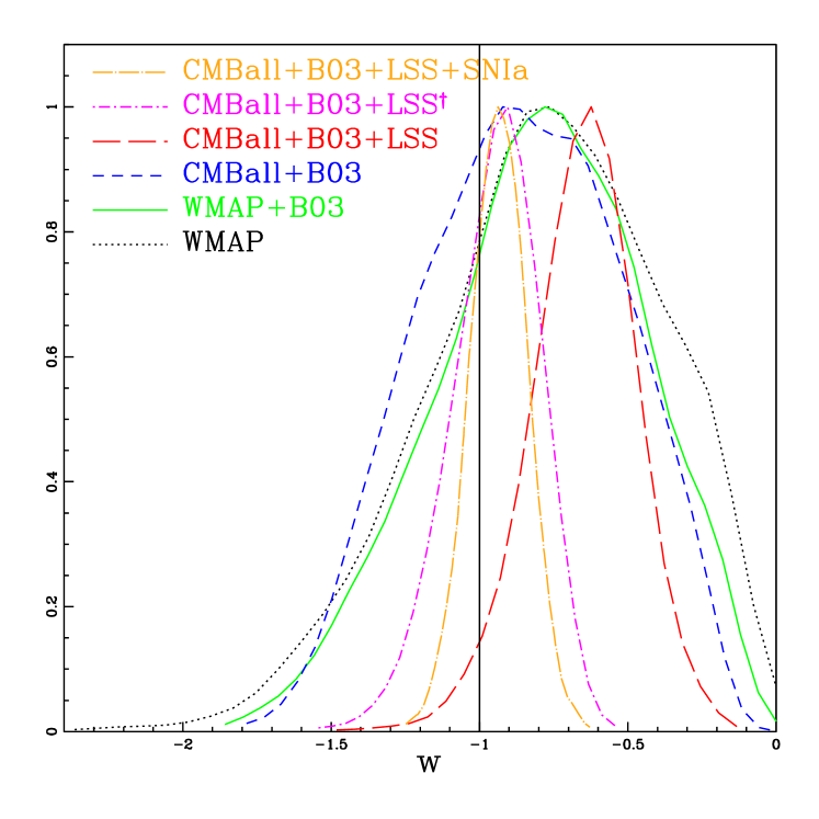
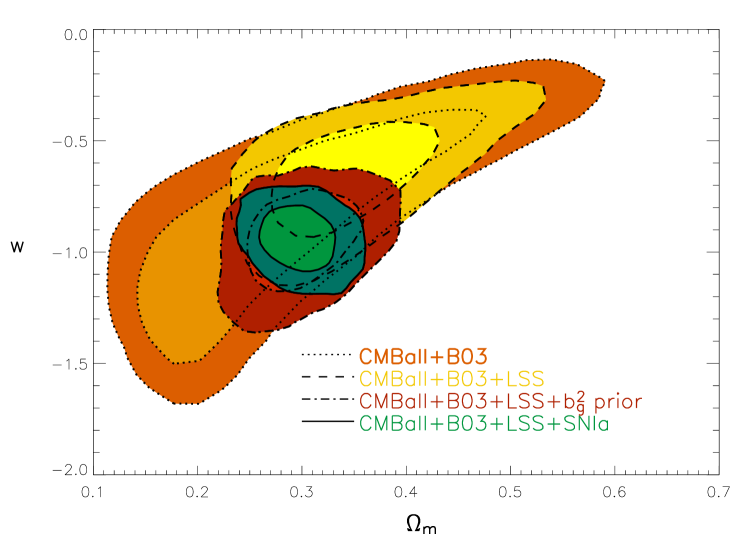
The standard model predicts (and CMB observations strongly support) a universe which is nearly flat, implying a total energy density approaching critical. The total matter density however, comprises only one third of the total energy density. The prevailing energy density component comes from some form of dark energy which up to now we have assumed takes the form of a vacuum density or cosmological constant, $\Lambda$, with equation of state described by $w=p/\rho=-1$, where $p$ and $\rho$ are the dark energy pressure and density respectively. We now consider the possibility that the dark energy component is a rolling scalar field or quintessence (see for example Ratra & Peebles (1988) or Huey et al. (1999)), allowing the effective constant equation of state parameter $w$ to differ from $-1$. We treat $w$ as a redshift-independent phenomenological factor and allow it to range with a uniform prior over the range $-4$ to $0$. We have also run the cases with $w$ restricted to lie in the range $-1$ to $0$ and find similar limits. To be self-consistent, perturbations in the dark energy should be allowed for when $w$ is not $-1$, although these have a small impact and only at low multipoles. We set the effective sound speed for the perturbations to unity in camb, the value for a scalar field.

The marginalized one-dimensional distributions for various data combinations are presented in Figure 10. We find from CMB data alone $w=-0.86^{+0.36}_{-0.35}$. The addition of the LSS data, applying the conservative uniform flat prior on $b_{g}^{2}$ to the galaxy bias factor, yields a median value of $w=-0.65\pm 0.16$. This result is highly sensitive to our choice of prior on $b_{g}^{2}$. The uniform flat prior on $b_{g}^{2}$ gives a relatively high best fit bias value of $b_{g}=1.3$. Applying a more restrictive Gaussian prior to $b_{g}^{2}$ gives: $w=-0.95\pm 0.15$ with $b_{g}=1.0\pm 0.10$; and $w=-0.75\pm 0.15$ with $b_{g}=1.0\pm 0.50$. We explore the effect of adding the SNIa data which significantly improves the constraint on $w$ yielding $w=-0.94^{+0.094}_{-0.096}$ with the flat prior on $b_{g}^{2}$. Results for the CMBall+B03 data set and the CMBall+B03+LSS+SNIa data set are given in Table 5.

Figure 10 illustrates the degeneracy in the $\Omega_{m}-w$ plane that cannot be broken by CMB data alone and is only weakly broken with the addition of the LSS data (flat prior on $b_{g}^{2}$). Application of a more restrictive Gaussian prior to $b_{g}^{2}$ for the LSS data or addition of the SNIa data breaks the degeneracy.

Figure 9: Marginalized one-dimensional distributions for the dark matter equation of state parameter $w$. Weak priors imposed on the base parameters are those outlined in Table 2. We also impose the prior $-4<w<0$. The $\dagger$ denotes the application of a Gaussian prior to $b_{g}^{2}$ (with $b_{g}=1\pm 10\%$). The nominal flat uniform prior on $b_{g}^{2}$ yields a slightly higher median value for $w$, driven by higher values of $b_{g}$. Adding the SNIa data however, reduced the median value to $-0.94\pm 0.1$.

Figure 10: Constraints on $w$ versus $\Omega_{m}$ for a flat $\Lambda$CDM model that allows the dark energy equation of state parameter, $w$, to differ from -1. Inner contours represent 68% likelihood regions and outer contours 95% likelihood regions. A more stringent Gaussian $b_{g}^{2}$ prior (with $b_{g}=1\pm 10\%$) or the addition of SNIa data is required to break the strong geometric degeneracy.

Table 5: Marginalized parameter constraints for five modifications of the baseline model. Parameter uncertainties represent the 68% confidence interval. For the case of upper or lower bounds 95% confidence limits are quoted. The following flat weak priors are imposed on the base 6 parameters (as outlined in Table 2): $0.5\leq n_{s}\leq 1.5$; $2.7\leq\ln(10^{10}A_{s})\leq 4.0$; $0.005\leq\Omega_{b}h^{2}\leq 0.1$; $0.01\leq\Omega_{c}h^{2}\leq 0.99$; $0.5\leq\theta\leq 10.0$; and $0.01\leq\tau\leq 0.8$. Additional weak priors restrict the age of the universe to $10\text{Gyr}\leq\text{age}\leq 20\text{Gyr}$ and the expansion rate to $45\leq H_{0}\leq 90$. We add, in turn, one parameter to the base set and impose the following prior on each: running index, $-0.3<{n_{\rm run}}<0.3$; curvature, $-0.3<\Omega_{k}<0.3$ ; amplitude ratio, $0<A_{\rm t}/A_{\rm s}<20$; neutrino fraction of dark matter, $0<f_{\nu}<1$; and dark energy equation of state, $-4<w<0$. The CMBall data set is as given in Table 3. The LSS data consists of the matter power spectra from the 2dFGRS and SDSS redshift surveys. We have marginalized the galaxy bias factor $b_{g}$ assuming a uniform flat prior in $b_{g}^{2}$. For the $Base+w$ case only we add in both the LSS and SNIa data which gives a better constrained result than that which is obtained from adding LSS data alone. We include the baseline model results for comparison.

	Base+Running Index		Base+Curvature
	CMBall	CMBall	CMBall	CMBall
	+B03	+LSS+B03	+B03	+LSS+B03
$\Omega_{b}h^{2}$	$0.0238^{+0.0019}_{-0.0019}$	$0.0219^{+0.0010}_{-0.0010}$	$0.0231^{+0.0010}_{-0.0013}$	$0.0227^{+0.0009}_{-0.0010}$
$\Omega_{c}h^{2}$	$0.104^{+0.015}_{-0.013}$	$0.125^{+0.007}_{-0.007}$	$0.106^{+0.011}_{-0.011}$	$0.111^{+0.008}_{-0.008}$
$\theta$	$1.048^{+0.005}_{-0.005}$	$1.044^{+0.004}_{-0.004}$	$1.045^{+0.005}_{-0.005}$	$1.044^{+0.004}_{-0.004}$
$\tau$	$0.31^{+0.13}_{-0.14}$	$0.151^{+0.025}_{-0.036}$	$0.178^{+0.087}_{-0.092}$	$0.139^{+0.021}_{-0.129}$
$n_{\rm s}$	$0.95^{+0.06}_{-0.06}$	$0.90^{+0.04}_{-0.04}$	$0.97^{+0.03}_{-0.04}$	$0.96^{+0.02}_{-0.03}$
$\ln[10^{10}A_{\rm s}]$	$3.5^{+0.2}_{-0.3}$	$3.2^{+0.1}_{-0.1}$	$3.2^{+0.2}_{-0.2}$	$3.1^{+0.1}_{-0.1}$
$\Omega_{\Lambda}$	$0.78^{+0.07}_{-0.07}$	$0.67^{+0.04}_{-0.04}$	$0.67^{+0.12}_{-0.13}$	$0.67^{+0.05}_{-0.04}$
${\rm Age(Gyr)}$	$13.3^{+0.4}_{-0.4}$	$13.7^{+0.2}_{-0.2}$	$14.9^{+1.3}_{-1.3}$	$14.8^{+0.7}_{-0.7}$
$\Omega_{m}$	$0.22^{+0.07}_{-0.07}$	$0.33^{+0.04}_{-0.04}$	$0.37^{+0.17}_{-0.16}$	$0.36^{+0.05}_{-0.06}$
$\sigma_{8}$	$0.91^{+0.07}_{-0.07}$	$0.89^{+0.06}_{-0.06}$	$0.81^{+0.06}_{-0.06}$	$0.82^{+0.06}_{-0.06}$
$z_{re}$	$24.7^{+5.7}_{-6.4}$	$16.8^{+5.0}_{-5.0}$	$16.6^{+5.7}_{-5.5}$	$14.7^{+4.7}_{-4.7}$
$H_{0}$	$78.1^{+11.9}_{-8.7}$	$66.8^{+1.3}_{-1.5}$	$62.5^{+13.1}_{-17.5}$	$61.7^{+2.4}_{-2.1}$
${n_{\rm run}}$	$-0.072^{+0.036}_{-0.036}$	$-0.051^{+0.027}_{-0.026}$	-	-
$\Omega_{k}$	-	-	$-0.037^{+0.033}_{-0.039}$	$-0.027^{+0.016}_{-0.016}$
	Base+Tensor Modes		Base+Massive Neutrinos
	CMBall	CMBall	CMBall	CMBall
	+B03	+LSS+B03	+B03	+LSS+B03
$\Omega_{b}h^{2}$	$0.0246^{+0.0013}_{-0.0013}$	$0.0232^{+0.0009}_{-0.0009}$	$0.0226^{+0.0014}_{-0.0014}$	$0.0224^{+0.0008}_{-0.0009}$
$\Omega_{c}h^{2}$	$0.0957^{+0.0090}_{-0.0086}$	$0.117^{+0.006}_{-0.006}$	$0.120^{+0.014}_{-0.014}$	$0.126^{+0.007}_{-0.007}$
$\theta$	$1.048^{+0.004}_{-0.004}$	$1.046^{+0.004}_{-0.004}$	$1.047^{+0.005}_{-0.005}$	$1.045^{+0.004}_{-0.004}$
$\tau$	$0.162^{+0.072}_{-0.070}$	$0.104^{+0.049}_{-0.049}$	$0.164^{+0.094}_{-0.088}$	$0.108^{+0.049}_{-0.047}$
$n_{\rm s}$	$1.02^{+0.04}_{-0.04}$	$0.97^{+0.02}_{-0.02}$	$0.95^{+0.04}_{-0.04}$	$0.95^{+0.02}_{-0.02}$
$\ln[10^{10}A_{\rm s}]$	$3.1^{+0.1}_{-0.1}$	$3.1^{+0.1}_{-0.1}$	$3.2^{+0.2}_{-0.2}$	$3.1^{+0.1}_{-0.1}$
$\Omega_{\Lambda}$	$0.82^{+0.03}_{-0.04}$	$0.72^{+0.03}_{-0.03}$	$0.64^{+0.11}_{-0.11}$	$0.64^{+0.06}_{-0.05}$
${\rm Age(Gyr)}$	$13.2^{+0.3}_{-0.2}$	$13.5^{+0.2}_{-0.2}$	$14.1^{+0.4}_{-0.4}$	$13.9^{+0.2}_{-0.2}$
$\Omega_{m}$	$0.181^{+0.036}_{-0.034}$	$0.28^{+0.03}_{-0.03}$	$0.36^{+0.11}_{-0.11}$	$0.36^{+0.05}_{-0.06}$
$\sigma_{8}$	$0.77^{+0.07}_{-0.07}$	$0.84^{+0.05}_{-0.05}$	$0.60^{+0.13}_{-0.12}$	$0.74^{+0.08}_{-0.08}$
$z_{re}$	$15.2^{+4.5}_{-4.5}$	$12.2^{+4.0}_{-4.0}$	$16.6^{+6.2}_{-5.9}$	$13.0^{+4.1}_{-4.0}$
$H_{0}$	$>73.2$	$71.4^{+2.8}_{-2.9}$	$64.9^{+8.1}_{-7.4}$	$64.8^{+3.9}_{-3.8}$
$A_{\rm t}/A_{\rm s}$	$<0.71$	$<0.36$	-	-
$f_{\nu}$	-	-	$<0.21$	$<0.09$
	Base+w		Baseline
	CMBall	CMBall	CMBall	CMBall
	+B03	+LSS+B03+SNIa	+B03	+LSS+B03
$\Omega_{b}h^{2}$	$0.0234^{+0.0013}_{-0.0013}$	$0.0229^{+0.0009}_{-0.0009}$	$0.0233^{+0.0013}_{-0.0012}$	$0.0227^{+0.0008}_{-0.0008}$
$\Omega_{c}h^{2}$	$0.106^{+0.011}_{-0.011}$	$0.117^{+0.007}_{-0.008}$	$0.106^{+0.010}_{-0.010}$	$0.120^{+0.005}_{-0.005}$
$\theta$	$1.046^{+0.005}_{-0.005}$	$1.045^{+0.004}_{-0.004}$	$1.045^{+0.004}_{-0.004}$	$1.045^{+0.004}_{-0.004}$
$\tau$	$0.161^{+0.078}_{-0.077}$	$0.118^{+0.053}_{-0.055}$	$0.170^{+0.090}_{-0.081}$	$0.106^{+0.047}_{-0.048}$
$n_{\rm s}$	$0.98^{+0.04}_{-0.04}$	$0.96^{+0.02}_{-0.02}$	$0.98^{+0.04}_{-0.03}$	$0.95^{+0.02}_{-0.02}$
$\ln[10^{10}A_{\rm s}]$	$3.2^{+0.1}_{-0.1}$	$3.1^{+0.1}_{-0.1}$	$3.2^{+0.2}_{-0.2}$	$3.1^{+0.1}_{-0.1}$
$\Omega_{\Lambda}$	$0.71^{+0.10}_{-0.11}$	$0.70^{+0.02}_{-0.02}$	$0.77^{+0.05}_{-0.05}$	$0.70^{+0.03}_{-0.03}$
${\rm Age(Gyr)}$	$13.7^{+0.4}_{-0.4}$	$13.6^{+0.2}_{-0.2}$	$13.5^{+0.2}_{-0.3}$	$13.6^{+0.2}_{-0.2}$
$\Omega_{m}$	$0.29^{+0.11}_{-0.10}$	$0.30^{+0.02}_{-0.02}$	$0.23^{+0.05}_{-0.05}$	$0.30^{+0.03}_{-0.03}$
$\sigma_{8}$	$0.76^{+0.15}_{-0.15}$	$0.82^{+0.06}_{-0.06}$	$0.83^{+0.06}_{-0.06}$	$0.85^{+0.05}_{-0.05}$
$z_{re}$	$15.9^{+5.0}_{-4.9}$	$13.3^{+4.2}_{-4.2}$	$16.5^{+5.4}_{-5.1}$	$12.6^{+3.9}_{-4.0}$
$H_{0}$	$69.9^{+13.1}_{-12.9}$	$68.6^{+2.1}_{-2.0}$	$75.8^{+5.6}_{-5.1}$	$69.6^{+2.4}_{-2.4}$
$w$	$-0.86^{+0.36}_{-0.35}$	$-0.94^{+0.094}_{-0.096}$	-	-

5 Sub-dominant Isocurvature Model

CMB anisotropies provide a powerful probe of the nature of early universe perturbations. However almost any TT power spectrum shape can be fit rather well by using contrived combinations of initial perturbations, for example by adding structure to the primordial power spectrum, and/or by adding isocurvature modes (which come in many varieties). With full freedom, determination of the basic cosmic parameters suffers because of high correlation with these extra degrees of freedom. These degeneracies are broken by the addition of polarization data, because of the pattern differences of the peaks and troughs between EE, TE and TT power spectra. In particular the intensity and polarization power spectra for isocurvature modes have the peaks out of phase with those from adiabatic modes (see e.g., Bond & Efstathiou (1987), Hu et al. (1997)). A mix of isocurvature and adiabatic modes can be designed to give acceptable fits to the CMB intensity power spectra (e.g., (Bucher et al., 2004; Kurki-Suonio et al., 2005)), and the polarization data, from B03 as well from DASI, CAPMAP and CBI are not yet at the point to clearly distinguish among these more complex models.

To illustrate the constraints that can be determined from the current CMB data, we consider here a simple hybrid case consisting of our basic adiabatic mode model with constant spectral index, a single cold dark matter (CDM) isocurvature mode with its own constant primordial spectral index $n_{\rm iso}$, with no correlation between the two. This adds another two parameters to our basic six, $n_{\rm iso}$ and an amplitude ratio $R_{2}\equiv(A_{iso}/A_{\rm s})$. We assume the isocurvature perturbations are Gaussian-distributed as we have done for the adiabatic modes. Results are shown in Table 6 for the CMBall+B03+HST data combination. Aside from the more stringent HST data prior on $H_{0}$, all priors on the 6 base parameters are as outlined in Table 2. Although results indicate that there is no evidence for the presence of an isocurvature mode, the upper limits still allow for a sub-dominant component.

We now expand on the theoretical framework. Isocurvature modes may arise in two (or more) field models of inflation, and, though certainly not a natural prediction, they have reasonably good physical motivation. Isocurvature modes could also be generated after inflation ended. An ingredient needed for isocurvature modes to have an observable impact on the CMB is that they are associated with a component of significant mass-energy. If the dark matter is cold and of one type there are two distinct matter isocurvature modes, the baryon and CDM modes, involving primordial fluctuations in the entropy-per-baryon or the entropy-per-CDM-particle. The classic example of a CDM possibility is the isocurvature axion mode. It turns out that the isocurvature CDM and baryon modes actually have almost identical signatures in the CMB (Gordon & Lewis, 2003), and hence cannot be constrained separately. In this paper we choose to constrain only the CDM isocurvature mode. There are other possibilities for isocurvature modes that we will not explore here.

It is a straightforward modification of CosmoMC to include an additional isocurvature component in the MCMC chains, which uses camb to compute the isocurvature power spectra. Instead of using $n_{\rm iso}$ as a basic parameter, we use two amplitude ratios for the two parameters that characterize our CDM isocurvature mode, following a suggestion of Kurki-Suonio et al. (2005):

$$R_{2}\equiv{\cal P}_{\rm iso}(k_{2})/{\cal P}_{\rm s}(k_{2})\,,\ k_{2}=0.05\text{Mpc}^{-1},$$ (5)

$$R_{1}\equiv{\cal P}_{\rm iso}(k_{1})/{\cal P}_{\rm s}(k_{1}),\ k_{1}=0.005\text{Mpc}^{-1}\,.$$

Here ${\cal P}_{\rm s}(k)$ is the power in the primordial curvature perturbation and ${\cal P}_{\rm iso}(k)$ is the power in the primordial CDM-photon entropy perturbation. The $k_{2}$ scale corresponds to $\ell\sim 700$ and $k_{1}$ to $\ell\sim 70$. We adopt a uniform prior probability over the range 0 to 20 for $R_{1}$, and over 0 to 100 for $R_{2}$. The isocurvature spectral index $n_{\rm iso}$, defined by ${\cal P}_{\rm iso}(k)\propto k^{n_{\rm iso}}$, is now a derived parameter, expressible in terms of $R_{1}$, $R_{2}$ and the adiabatic spectral index $n_{\rm s}$, defined by ${\cal P}_{\rm s}(k)\propto k^{{n_{\rm s}}-1}$,

$$n_{\rm iso}=n_{\rm s}-1+\ln(R_{2}/R_{1})/\ln(k_{2}/k_{1})\,.$$ (6)

Two interesting limiting cases are the scale invariant $n_{\rm iso}=0$ spectrum with high spatial correlation and the $n_{\rm iso}=3$ “isocurvature seed” white noise spectrum with no spatial correlation.

The limits shown in Table  6 demonstrate that the large scale $R_{1}$, dominated by the WMAP data, is much better constrained at $<0.3$ than the small scale $R_{2}<2.3$, which B03 probes. This translates into a preference for steeper $n_{\rm iso}$ than the scale invariant value. Since for neither is there an indication of a non-zero value, just upper limits, the results are sensitive to the prior probabilities we assign them. Our choice of uniform prior for $R_{1}$ and $R_{2}$ is conservative in that the upper limits decrease with other choices, e.g., one uniform in $\ln(R_{i})$ (a non-informative prior), or one uniform in $n_{\rm iso}$ and $R_{2}$. The conservative choice actually downgrades the probability of steep $n_{\rm iso}$. (The B03pol data by itself only limits $R_{1}<17$ and $R_{2}<22$; the full B03 data gives $R_{1}<1.8$ and $R_{2}<5.3$.)

Further constraints on isocurvature modes arise from LSS since the shape of the isocurvature matter power spectrum differs in significant ways from the adiabatic one, but we do not consider those here.

The strongest constraints come from the low $\ell$ part of the spectrum. However, spectra that are significantly steeper than inflation-motivated nearly-scale-invariant ones are still allowed by the data. To focus attention on the role played by the new, high $\ell$ B03 results, we now fix $n_{\rm iso}$ at 3, the white noise ‘seed’ spectrum, the limiting case in which the isocurvature perturbations when created were uncorrelated spatially. The large angular scales are highly suppressed and the isocurvature peaks and troughs emerge looking somewhat like an $\ell$-shifted version of the adiabatic spectrum. The two spectra then test at what level interleaved isocurvature peaks are allowed by the CMB data. Results are shown in Table 6. To relate the $R_{2}<3.0$ limit to a more intuitive expression of what the CMBall+B03+HST data set data allows, we note that over a bandpower in $\ell$ from 75 to 1400, ${\cal C}_{B}^{TT({\rm iso})}/{\cal C}_{B}^{TT({\rm s})}\sim(0.005)R_{2}$, hence the upper limit corresponds to an allowed CMB contamination of this sub-dominant component of TT of only a few percent. Over a bandpower in $\ell$ from 150 to 1000 we find ${\cal C}_{B}^{EE(\rm iso)}/{\cal C}_{B}^{EE(\rm s)}\sim(0.008)R_{2}$, for the allowed EE isocurvature bandpower contamination. B03pol gives $R_{2}<58$. The full B03 data set including TT gives $R_{2}<9.5$.

Since the isocurvature models adopted for these tests are not especially well-motivated physically, we have also chosen not to apply the LSS prior to our results.

The $n_{\rm iso}=3,2$ illustration allows us to conclude that even with the errors on the EE and TE data, there is evidence against the isocurvature shifted pattern over the adiabatic pattern and only restricted room for an interleaved peak pattern, at a level below 50%. This test differs from the adiabatic-only peak/trough pattern shift using B03pol Fig.3 since there are no interleaved peaks and troughs in that case. Examination of the camb models obtained from the marginalized constraints in Table 6 reveals that the parameters chosen by CosmoMC adjust to make the adiabatic ${\cal C}_{\ell}^{\rm s}$ pattern compensate for the isocurvature ${\cal C}_{\ell}^{\rm iso}$ contamination.

Table 6: Marginalized parameter constraints for a model which includes both (dominant) adiabatic and (sub-dominant) isocurvature modes. Parameter uncertainties represent the 68% confidence interval. Upper bounds are 95% confidence limits. The flat weak priors are imposed on the base 6 parameters are as outlined in Table 2. The CMBall data set is defined in Table 3. We include the baseline model result (with the more stringent HST prior) for comparison. We consider two parameterizations for the isocurvature model. For the first (column two) we add two parameters to our basic six: $R_{2}\equiv{\cal P}_{\rm iso}(k_{2})/{\cal P}_{\rm s}(k_{2})$, with pivot scale $k_{2}=0.05\text{Mpc}^{-1}$; and $R_{1}\equiv{\cal P}_{\rm iso}(k_{1})/{\cal P}_{\rm s}(k_{1})$ with $k_{1}=0.005\text{Mpc}^{-1}$. We impose the priors $0<R_{1}<20$ and $0<R_{2}<100$. For this case the isocurvature spectral index, $n_{\rm iso}$, is a derived parameter. We also consider the “white isocurvature” case (column three) where we fix $n_{\rm iso}=3$ and allow the amplitude ratio $R_{2}\equiv(A_{\rm iso}/A_{\rm s})$ to lie anywhere between 0 and 100.

	Baseline	Adiabatic + Iso	Adiabatic + White Iso
	CMBall	CMBall	CMBall
	+B03+HST	+B03+HST	+B03+HST
$\Omega_{b}h^{2}$	$0.0230^{+0.0010}_{-0.0010}$	$0.0247^{+0.0014}_{-0.0014}$	$0.0235^{+0.0012}_{-0.0011}$
$\Omega_{c}h^{2}$	$0.108^{+0.008}_{-0.008}$	$0.103^{+0.009}_{-0.009}$	$0.107^{+0.009}_{-0.009}$
$\theta$	$1.045^{+0.004}_{-0.004}$	$1.051^{+0.005}_{-0.005}$	$1.046^{+0.005}_{-0.005}$
$\tau$	$0.151^{+0.069}_{-0.067}$	$0.163^{+0.071}_{-0.069}$	$0.156^{+0.071}_{-0.071}$
$n_{\rm s}$	$0.97^{+0.03}_{-0.03}$	$1.01^{+0.04}_{-0.04}$	$0.97^{+0.03}_{-0.03}$
$R_{1}$	$-$	$<0.28$	$-$
$R_{2}$	$-$	$<2.3$	$<3.0$
$n_{\rm iso}$	$-$	$1.1^{+0.6}_{-0.5}$	$3.0(fixed)$
$\ln[10^{10}A_{\rm s}]$	$3.1^{+0.1}_{-0.1}$	$3.2^{+0.1}_{-0.1}$	$3.1^{+0.1}_{-0.1}$
$\Omega_{\Lambda}$	$0.76^{+0.04}_{-0.04}$	$0.80^{+0.04}_{-0.04}$	$0.77^{+0.04}_{-0.04}$
${\rm Age(Gyr)}$	$13.5^{+0.2}_{-0.2}$	$13.1^{+0.3}_{-0.3}$	$13.4^{+0.2}_{-0.2}$
$\Omega_{m}$	$0.24^{+0.04}_{-0.04}$	$0.20^{+0.04}_{-0.04}$	$0.23^{+0.04}_{-0.04}$
$z_{re}$	$15.4^{+4.7}_{-4.5}$	$15.5^{+4.4}_{-4.4}$	$15.6^{+4.8}_{-4.6}$
$H_{0}$	$74.4^{+4.0}_{-3.9}$	$80.3^{+5.6}_{-5.5}$	$75.9^{+4.3}_{-4.2}$

6 Conclusions

The B03 data set does well at constraining the cosmological parameters of the standard $\Lambda$CDM model. The results are in good agreement with those derived from other CMB experiments, as is evident in Table 4. The parameter constraints derived from the B03 data set in combination with the WMAP data are highly competitive with those from the CMBall data set.

We have applied the Slosar-Seljak modification to the WMAP data which has the general effect of broadening slightly the WMAP 1D likelihood curves with the largest impacts on the (WMAP alone) median values of $\tau$ ($\sim 0.3\sigma$ increase) and $\Omega_{m}$ ($\sim 0.6\sigma$ decrease) for the baseline model and ${n_{\rm run}}$ ($\sim 0.5\sigma$ increase) for the baseline+running index model. Our graphical representation of the standard model parameters in Figure 2 illustrates the impact of the addition of the LSS data, which shifts the median values very little. Figure 2 shows the best estimates for the parameters of the $\Lambda$CDM model from current CMB and LSS redshift survey data.

Our analysis of five extensions to the standard model is summarized in Table 5. Intriguingly we found two cases, the running index and neutrino fraction, where the addition of data from higher multipole CMB experiments drove median values away from the conventional value. The evidence for a running index however, is slight ($<2\sigma$). Our neutrino mass limit (assuming three species of nearly degenerate mass) from CMB data alone is $m_{\nu}<1.0{\,\rm eV}$ and from the combined CMB and LSS data set is $m_{\nu}<0.40{\,\rm eV}$, with no $b_{g}$ prior, and $m_{\nu}<0.16{\,\rm eV}$, with $b_{g}=1.0\pm 0.10$.

We have explored the sensitivity of our CMBall+B03+LSS results to the prior imposed on the galaxy bias factor $b_{g}$ and have found that only the neutrino mass results (above) and dark energy equation of state results are significantly impacted. For the dark energy equation of state we find that applying a more restrictive Gaussian prior to $b_{g}^{2}$ gives $w=-0.97\pm 0.12$ with $b_{g}=1.0\pm 0.10$. Without any $b_{g}$ constraint we find $w=-0.65\pm 0.16$. However, addition of the SNIa data, with the flat prior on $b_{g}^{2}$, yields $w=-0.94^{+0.094}_{-0.096}$. The results are consistent with the dark energy being the cosmological constant.

While the polarization data is not yet at the level of accuracy of the intensity data, cross checks of best fit parameters from the B03pol data and B03TT data indicate consistent results. The consistency of the shape parameter $\theta$ determined from B03pol and from B03TT demonstrates that the peak and trough positions forecast by the spectra are in robust agreement. Isocurvature modes are beginning to be constrained by the current CMB polarization data and our upper limits and phenomenological discussion represent a good starting point for future analysis of these more complex models. The CMB polarization data is emerging but is not yet driving parameter determination. We look forward to future higher precision data in which polarization data will play a larger role.

References

- Ahmad et al. (2002) Ahmad, Q. R. et al. 2002, Phys. Rev. Lett., 89, 011301
- Aliani et al. (2003) Aliani, P., Antonelli, V., Picariello, M., & Torrente-Lujan, E. 2003, hep-ph/0309156
- Bond et al. (2004) Bond, J. R., Contaldi, C. R., Lewis, A. M., & Pogosyan, D. 2004, Int. J. Theor. Phys., 43, 599
- Bond et al. (2003) Bond, J. R., Contaldi, C. R., & Pogosyan, D. 2003, Phil. Trans. Roy. Soc. Lond., A361, 2435
- Bond & Efstathiou (1987) Bond, J. R. & Efstathiou, G. 1987, Mon. Not. Roy. Astron. Soc., 226, 655
- Bond et al. (1997) Bond, J. R., Efstathiou, G., & Tegmark, M. 1997, Mon. Not. Roy. Astron. Soc., 291, L33
- Bond et al. (2000) Bond, J. R., Jaffe, A. H., & Knox, L. E. 2000, Astrophys. J., 533, 19
- Bond et al. (2005) Bond, J. R. et al. 2005, Astrophys. J., 626, 12
- Bucher et al. (2004) Bucher, M., Dunkley, J., Ferreira, P. G., Moodley, K., & Skordis, C. 2004, astro-ph/0401417
- Bucher et al. (2000) Bucher, M., Moodley, K., & Turok, N. 2000, Phys. Rev., D62, 083508
- Chon et al. (2004) Chon, G., Challinor, A., Prunet, S., Hivon, E., & Szapudi, I. 2004, Mon. Not. Roy. Astron. Soc., 350, 914
- Christensen et al. (2001) Christensen, N., Meyer, R., Knox, L., & Luey, B. 2001, Class. Quant. Grav., 18, 2677
- Cole et al. (2005) Cole, S. et al. 2005, astro-ph/0501174
- Contaldi et al. (2005) Contaldi, C. et al. 2005, in prep
- Contaldi et al. (2003) Contaldi, C. R., Hoekstra, H., & Lewis, A. 2003, Phys. Rev. Lett., 90, 221303
- de Bernardis et al. (2000) de Bernardis, P. et al. 2000, Nature, 404, 955
- Dickinson et al. (2004) Dickinson, C. et al. 2004, astro-ph/0402498
- Dore et al. (2004) Dore, O., Holder, G. P., & Loeb, A. 2004, Astrophys. J., 612, 81
- Efstathiou & Bond (1986) Efstathiou, G. & Bond, J. R. 1986, MNRAS, 218, 103
- Eidelman et al. (2004) Eidelman, S. et al. 2004, Physics Letters B, 592, 1+
- Eisenstein et al. (2005) Eisenstein, D. J. et al. 2005, astro-ph/0501171
- Freedman et al. (2001) Freedman, W. L. et al. 2001, Astrophys. J., 553, 47
- Frigo & Johnson (2005) Frigo, M. & Johnson, S. G. 2005, Proceedings of the IEEE, 93, 216
- Gordon & Lewis (2003) Gordon, C. & Lewis, A. 2003, Phys. Rev., D67, 123513
- Gorski et al. (2005) Gorski, K. M. et al. 2005, Astrophys. J., 622, 759
- Halverson et al. (2002) Halverson, N. W. et al. 2002, Astrophys. J., 568, 38
- Hanany et al. (2000) Hanany, S. et al. 2000, Astrophys. J., 545, L5
- Hedman et al. (2002) Hedman, M. M. et al. 2002, astro-ph/0204438
- Hinshaw et al. (2003) Hinshaw, G. et al. 2003, Astrophys. J. Suppl., 148, 135
- Hivon et al. (2001) Hivon, E. et al. 2001, astro-ph/0105302
- Hu et al. (1997) Hu, W., Sugiyama, N., & Silk, J. 1997, Nature, 386, 37
- Huey et al. (1999) Huey, G., Wang, L., Dave, R., Caldwell, R. R., & Steinhardt, P. J. 1999, Phys. Rev., D59, 063005
- Jones et al. (2005a) Jones, W. et al. 2005a, in prep
- Jones et al. (2005b) —. 2005b, submitted to ApJ
- Kogut et al. (2003) Kogut, A. et al. 2003, Astrophys. J. Suppl., 148, 161
- Kosowsky et al. (2002) Kosowsky, A., Milosavljevic, M., & Jimenez, R. 2002, Phys. Rev. D., 66, 063007
- Kosowsky & Turner (1995) Kosowsky, A. & Turner, M. S. 1995, Phys. Rev., D52, 1739
- Kovac et al. (2002) Kovac, J. et al. 2002, Nature, 420, 772
- Kuo et al. (2004) Kuo, C.-l. et al. 2004, Astrophys. J., 600, 32
- Kurki-Suonio et al. (2005) Kurki-Suonio, H., Muhonen, V., & Valiviita, J. 2005, Phys. Rev., D71, 063005
- Lange et al. (2001) Lange, A. E. et al. 2001, Phys. Rev., D63, 042001
- Lewis (2004) Lewis, A. 2004, Phys. Rev., D70, 043518
- Lewis & Bridle (2002) Lewis, A. & Bridle, S. 2002, Phys. Rev., D66, 103511
- Lewis et al. (2000) Lewis, A., Challinor, A., & Lasenby, A. 2000, Astrophys. J., 538, 473
- Masi et al. (2005) Masi, S. et al. 2005, submitted to ApJ
- McDonald et al. (2004) McDonald, P. et al. 2004, astro-ph/0405013
- Montroy et al. (2005) Montroy, T. et al. 2005, submitted to ApJ
- Neal (1993) Neal, R. M. 1993, http://www.cs.toronto.edu/radford/review.abstract.html
- Netterfield et al. (2002) Netterfield, C. B. et al. 2002, Astrophys. J., 571, 604
- Percival et al. (2001) Percival, W. J. et al. 2001, MNRAS, 327, 1297
- Piacentini et al. (2005) Piacentini, F. et al. 2005, submitted to ApJ
- Ratra & Peebles (1988) Ratra, B. & Peebles, P. J. E. 1988, Phys. Rev., D37, 3406
- Readhead et al. (2004a) Readhead, A. C. S. et al. 2004a, Astrophys. J., 609, 498
- Readhead et al. (2004b) —. 2004b, Science, 306, 836
- Rebhan & Schwarz (1994) Rebhan, A. K. & Schwarz, D. J. 1994, Phys. Rev., D50, 2541
- Riess et al. (2004) Riess, A. G. et al. 2004, Astrophys. J., 607, 665
- Ruhl et al. (2003) Ruhl, J. E. et al. 2003, Astrophys. J., 599, 786
- Seljak & Zaldarriaga (1996) Seljak, U. & Zaldarriaga, M. 1996, Astrophys. J., 469, 437
- Seljak et al. (2004) Seljak, U. et al. 2004, astro-ph/0407372
- Seljak et al. (2005) —. 2005, Phys. Rev., D71, 043511
- Slosar et al. (2004) Slosar, A., Seljak, U., & Makarov, A. 2004, Phys. Rev., D69, 123003
- Spergel et al. (2003) Spergel, D. N. et al. 2003, Astrophys. J. Suppl., 148, 175
- Tegmark et al. (2003) Tegmark, M. et al. 2003, astro-ph/0310725
- Toshito et al. (2001) Toshito, T. et al. 2001, hep-ex/0105023
- Tristram et al. (2005) Tristram, M. et al. 2005, Astron. Astrophys., 436, 785
- Verde et al. (2002) Verde, L. et al. 2002, Mon. Not. Roy. Astron. Soc., 335, 432
- Verde et al. (2003) —. 2003, Astrophys. J. Suppl., 148, 195