Heavy element abundances in DAO white dwarfs measured from FUSE data

Abstract

We present heavy element abundance measurements for 16 DAO white dwarfs, determined from Far-Ultraviolet Spectroscopic Explorer (FUSE) spectra. Evidence of absorption by heavy elements was found in the spectra of all the objects. Measurements were made using models that adopted the temperatures, gravities and helium abundances determined from both optical and FUSE data by Good et al. (2004). It was found that, when using the values for those parameters measured from optical data, the carbon abundance measurements follow and extend a similar trend of increasing abundance with temperature for DA white dwarfs, discovered by Barstow et al. (2003). However, when the FUSE measurements are used the DAO abundances no longer join this trend since the temperatures are higher than the optical measures. Silicon abundances were found to increase with temperature, but no similar trend was identified in the nitrogen, oxygen, iron or nickel abundances, and no dependence on gravity or helium abundances were noted. However, the models were not able to reproduce the observed silicon and iron line strengths satisfactorily in the spectra of half the objects, and the oxygen features of all but three. Despite the different evolutionary paths that the types of DAO white dwarfs are thought to evolve through, their abundances were not found to vary significantly, apart from for the silicon abundances.

Abundances measured when the FUSE derived values of temperature, gravity and helium abundance were adopted were, in general, a factor 1-10 higher than those determined when the optical measure of those parameters was used. Satisfactory fits to the absorption lines were achieved in approximately equal number. The models that used the FUSE determined parameters seemed better at reproducing the strength of the nitrogen and iron lines, while for oxygen, the optical parameters were better. For the three objects whose temperature measured from FUSE data exceeds 120 000 K, the carbon, nitrogen and oxygen lines were too weak in the models that used the FUSE parameters. However, the model that used the optical parameters also did not reproduce the strength of all the lines accurately.

1 Introduction

DAO white dwarfs, for which the prototype is HZ 34 (Koester, Weidemann, & Schulz, 1979; Wesemael et al., 1993), are characterised by the presence of He ii absorption in their optical spectra in addition to the hydrogen Balmer series. Radiative forces cannot support sufficient helium in the line forming region of the white dwarf to reproduce the observed lines (Vennes et al., 1988), and one explanation for their existence is that they are transitional objects switching between the helium- and hydrogen-rich cooling sequences (Fontaine & Wesemael, 1987). If a small amount of hydrogen were mixed into an otherwise helium dominated atmosphere, gravitational settling would then create a thin hydrogen layer at the surface of the white dwarf, with the boundary between the hydrogen and helium described by diffusive equilibrium. However, Napiwotzki & Schönberner (1993) found that the line profile of the He ii line at 4686 Å in the DAO S 216 was better matched by homogeneous composition models, rather than the predicted layered configuration. Subsequently, a spectroscopic investigation by Bergeron et al. (1994) found that the He ii line profile of only one out of a total of 14 objects was better reproduced by stratified models. In addition, the line profile of one object (PG 1210+533) could not be reproduced satisfactorily by either set of models.

Most of the DAOs analysed by Bergeron et al. were comparatively hot for white dwarfs, but with low gravity, which implies that they have low mass. Therefore, they may have not have been massive enough to ascend the asymptotic giant branch, and instead may have evolved from the extended horizontal branch. Bergeron et al. (1994) suggested that a process such as weak mass loss may be occurring in these stars, which might support the observed quantities of helium in the line forming regions of the DAOs (Unglaub & Bues, 1998, 2000). Three of the Bergeron et al. (1994) objects (RE 1016-053, PG 1413+015 and RE 2013+400) had comparatively ‘normal’ temperatures and gravities, yet helium absorption features were still observed. Each of these are in close binary systems with M dwarf (dM) companions. It may be that as the white dwarf progenitor passes through the common envelope phase, mass is lost, leading to the star being hydrogen poor. Then, a process such as weak mass loss could mix helium into the line forming region of the white dwarf. Alternatively, these DAOs might be accreting from the wind of their companions, as is believed to be the case for another DAO+dM binary, RE 0720-318 (Dobbie et al., 1999).

Knowledge of the effective temperature ($T_{\mathrm{eff}}$) and surface gravity (g) of a white dwarf is vital to our understanding of its evolutionary status. Values for both these parameters can be found by comparing the profiles of the observed hydrogen Balmer lines to theoretical models. This technique was pioneered by Holberg et al. (1985) and extended to a large sample of white dwarfs by Bergeron, Saffer, & Liebert (1992). However, for objects in close binary systems, where the white dwarf cannot be spatially resolved, the Balmer line profiles cannot be used as they are frequently contaminated by flux from the secondary (if it is of type K or earlier). Instead, the same technique can be applied to the Lyman lines that are found in far-ultraviolet (far-UV) data, as the white dwarf is much brighter in this wavelength region than the companion (e.g. Barstow et al., 1994). However, Barstow et al. (2001), Barstow et al. (2003) and Good et al. (2004) have compared the results of fitting the Balmer and Lyman lines of DA and DAO white dwarfs, and found that above 50 000 K, the $T_{\mathrm{eff}}$ measurements begin to diverge. This effect was stronger in some stars; in particular, the Lyman lines of 3 DAOs in the sample of Good et al. (2004) were so weak that the temperature of the best fitting model exceeded 120 000 K, which was the limit of their model grid.

One factor that influences the measurements of temperature and gravity is the treatment of heavy element contaminants in the atmosphere of a white dwarf. Barstow, Hubeny, & Holberg (1998) found that heavy element line blanketing significantly affected the Balmer line profiles in their theoretical models. The result was a decrease in the measured $T_{\mathrm{eff}}$ of a white dwarf compared to when a pure hydrogen model was used. In addition, Barstow et al. (2003) conducted a systematic set of measurements of the abundances of heavy elements in the atmospheres of hot DA white dwarfs, which differ from the DAOs in that no helium is observed. They found that the presence or lack of heavy elements in the photosphere of the white dwarfs largely reflected the predictions of radiative levitation, although the abundances did not match the expected values very well.

We have performed systematic measurements of the heavy element abundances in Far-Ultraviolet Spectroscopic Explorer (FUSE) observations of DAO white dwarfs. The motivation for this work was twofold: firstly, we wish to investigate if the different evolutionary paths suggested for the DAOs are reflected in their heavy element abundances, as compared to the DAs of Barstow et al. (2003). Secondly, since $T_{\mathrm{eff}}$ and log $g$ measurements from both optical and far-UV data for all the DAOs in our sample have previously been published (Good et al., 2004), we investigate which set of models better reproduces the strengths of the observed lines. The paper is organised as follows: in §2, §3 and §4 we describe the observations, models and data analysis technique used. Then, in §5 the results of the abundance measurements are shown. The ability of the models to reproduce the observations are discussed in §6 and finally the conclusions are presented in §7.

2 Observations

Far-UV data for all the objects were obtained by the FUSE spectrographs and cover the full Lyman series, apart from Lyman $\alpha$. Table 1 summarizes the observations, which were downloaded by us from the Multimission Archive (http://archive.stsci.edu/mast.html), hosted by the Space Telescope Science Institute. Overviews of the FUSE mission and in-orbit performance can be found in Moos et al. (2000) and Sahnow et al. (2000) respectively. Full details of our data extraction, calibration and co-addition techniques are published in Good et al. (2004). In brief, the data are calibrated using the calfuse pipeline version 2.0.5 or later, resulting in eight spectra (covering different wavelength segments) per FUSE exposure. The exposures for each segment are then co-added, weighting each according to exposure time, and finally the segments are combined, weighted by their signal-to-noise, to produce a single spectrum. Before each co-addition, the spectra are cross-correlated and shifted to correct for any wavelength drift. Figure 1 shows an example of the output from this process, for PG 1210+533.

Table 1: List of FUSE observations for the stars in the sample. All observations used TTAG mode.

Object	WD number	Obs. ID	Date	Exp. Time (s)	Aperture
PN A66 7	WD0500-156	B0520901	2001/10/05	11525	LWRS
HS 0505+0112	WD0505+012	B0530301	2001/01/02	7303	LWRS
PN PuWe 1	WD0615+556	B0520701	2001/01/11	6479	LWRS
		S6012201	2002/02/15	8194	LWRS
RE 0720-318	WD0718-316	B0510101	2001/11/13	17723	LWRS
TON 320	WD0823+317	B0530201	2001/02/21	9378	LWRS
PG 0834+500	WD0834+501	B0530401	2001/11/04	8434	LWRS
PN A66 31		B0521001	2001/04/25	8434	LWRS
HS 1136+6646	WD1136+667	B0530801	2001/01/12	6217	LWRS
		S6010601	2001/01/29	7879	LWRS
Feige 55	WD1202+608	P1042105	1999/12/29	19638	MDRS
		P1042101	2000/02/26	13763	MDRS
		S6010101	2002/01/28	10486	LWRS
		S6010102	2002/03/31	11907	LWRS
		S6010103	2002/04/01	11957	LWRS
		S6010104	2002/04/01	12019	LWRS
PG 1210+533	WD1210+533	B0530601	2001/01/13	4731	LWRS
LB 2	WD1214+267	B0530501	2002/02/14	9197	LWRS
HZ 34	WD1253+378	B0530101	2003/01/16	7593	LWRS
PN A66 39		B0520301	2001/07/26	6879	LWRS
RE 2013+400	WD2011+395	P2040401	2000/11/10	11483	LWRS
PN DeHt 5	WD2218+706	A0341601	2000/08/15	6055	LWRS
GD 561	WD2342+806	B0520401	2001/09/08	5365	LWRS

Figure 1: FUSE spectrum of PG 1210+533, produced by combining the spectra from the individual detector segments. * The emission in the core of the Lyman beta H i line is due to terrestrial airglow.

3 Model calculations

A new grid of stellar model atmospheres was created using the non-local thermodynamic (non-LTE) code tlusty (v. 195) (Hubeny & Lanz, 1995) and its associated spectral synthesis code synspec (v. 45), based on the models created by Barstow et al. (2003); as with their models, all calculations were performed in non-LTE with full line-blanketing, and with a treatment of Stark broadening in the structure calculation. Grid points with varying abundances were calculated for 8 different temperatures between 40 000 and 120 000 K, in 10 000 K steps, 4 different values of log $g$: 6.5, 7.0, 7.5 and 8.0, and, since the objects in question are DAOs, 5 values of log $\frac{He}{H}$ between -5 and -1, in steps of 1. Therefore, the grid encompassed the full range of the stellar parameters determined for the DAOs by Good et al. (2004). Models were calculated for a range of heavy element abundances, which were factors of 10^-1 to 10^1.5 times the values found for the well studied white dwarf G 191-B2B in an earlier analysis (Barstow et al., 2001) (C/H = 4.0 $\times$ 10^-7, N/H = 1.6 $\times$ 10^-7, O/H = 9.6 $\times$ 10^-7, Si/H = 3.0 $\times$ 10^-7, Fe/H = 1.0 $\times$ 10^-5 and Ni/H = 5.0 $\times$ 10^-7), with each point a factor of 10^0.5 different from the adjacent point. Above this value it was found that the tlusty models did not converge. Since, even with these abundances, the observed strengths of some lines could not be reproduced, the range was further extended upwards by a factor of 10, using synspec. However, as scaling abundances in this way is only valid if it can be assumed that the structure of the white dwarf atmosphere will not be significantly affected by the change, abundance values this high should be treated with caution.

Molecular hydrogen is observed in the spectra of some the objects. For those stars, the templates of McCandliss (2003) were used with the measurements of Good et al. (2004) to create appropriate molecular hydrogen absorption spectra.

4 Data analysis

The measurements of heavy element abundances were performed using the spectral fitting program xspec (Arnaud, 1996), which adopts a $\chi^{2}$ minimisation techique to determine the set of model parameters that best matches a data set. As the full grid of synthetic spectra was large, it was split into 4 smaller grids, one for each value of log $g$. The FUSE spectrum for each white dwarf was split into sections, each containing absorption lines due to a single element. Table 2 lists the wavelength ranges used and the main species in those regions. Where absorption due to another element could not be avoided, the affected region was set to be ignored by the fitting process. The appropriate model grid for the object’s log $g$ was selected, from the measurements of Good et al. (2004), and the $T_{\mathrm{eff}}$ and helium abundance were constrained to fall within the 1$\sigma$ limits from the same measurements, but were allowed to vary freely within those ranges. For those stars whose spectra exhibit molecular hydrogen absorption, the molecular hydrogen model created for that object was also included. Then, the model abundance that best matched the absorption features in the real data was found, and 3$\sigma$ errors calculated from the $\Delta\chi^{2}$ distribution. Where an element was not detected, the 3$\sigma$ upper bound was calculated instead. This analysis was repeated separately for the parameters determined by Good et al. (2004) from both optical and FUSE data – these parameters are listed in Table 3.

Table 2: Wavelength regions chosen for spectral fitting, the main species in each range and the central wavelengths of strong lines.

Species	Wavelength range / Å		Central wavelengths / Å
C iv	1107.0 –	1108.2	1107.6, 1107.9, 1108.0
	1168.5 –	1170.0	1168.8, 1169.0
N iii	990.5 –	992.5	991.6
N iv	920.0 –	926.0	992.0, 922.5, 923.1,
			923.2, 923.7, 924.3
O iv	1067.0 –	1069.0	1067.8
O vi	1031.0 –	1033.0	1031.9
	1036.5 –	1038.5	1037.6
Si iii	1113.0 –	1114.0	1113.2
Si iv	1066.0 –	1067.0	1066.6, 1066.7
	1122.0 –	1129.0	1122.5, 1128.3
Fe v	1113.5 –	1115.5	1114.1
Fe vi/vii	1165.0 –	1167.0	1165.1, 1165.7,1166.2
Fe vii	1116.5 –	1118.0	1117.6
Ni v	1178.0 –	1180.0	1178.9

Table 3: Mean best fitting parameters obtained from optical and FUSE data, from Good et al. (2004). Log $\mathrm{\frac{He}{H}}$ is not listed for the optical data of PG 1210+533 as it is seen to vary between observations. 1$\sigma$ confidence intervals are given, apart from where the temperature or gravity of the object is beyond the range of the model grid and hence a $\chi^{2}$ minimum has not been reached. Where a parameter is beyond the range of the model grid, the value is written in italics. The final columns show the total molecular hydrogen column density for each star, where it was detected, and the measured interstellar extinction, also from Good et al. (2004).

	BALMER LINE SPECTRA			LYMAN LINE SPECTRA
Object	$T_{\mathrm{eff}}$ / K	Log $g$	Log $\mathrm{\frac{He}{H}}$	$T_{\mathrm{eff}}$ / K	Log $g$	Log $\mathrm{\frac{He}{H}}$	Log H2	E(B-V)
PN A66 7	66955 $\pm$3770	7.23 $\pm$0.17	-1.29 $\pm$0.15	99227 $\pm$2296	7.68 $\pm$0.06	-1.70 $\pm$0.09	18.5	0.001
HS 0505+0112	63227 $\pm$2088	7.30 $\pm$0.15	-1.00	120000	7.24	-1.00		0.047
PN PuWe 1	74218 $\pm$4829	7.02 $\pm$0.20	-2.39 $\pm$0.37	109150 $\pm$11812	7.57 $\pm$0.22	-2.59 $\pm$0.75	19.9	0.090
RE 0720-318	54011 $\pm$1596	7.68 $\pm$0.13	-2.61 $\pm$0.19	54060 $\pm$ 776	7.84 $\pm$0.03	-4.71 $\pm$0.69		0.019
TON 320	63735 $\pm$2755	7.27 $\pm$0.14	-2.45 $\pm$0.22	99007 $\pm$4027	7.26 $\pm$0.07	-2.00 $\pm$0.12	14.9	0.000
PG 0834+500	56470 $\pm$1651	6.99 $\pm$0.11	-2.41 $\pm$0.21	120000	7.19	-5.00	18.2	0.033
PN A66 31	74726 $\pm$5979	6.95 $\pm$0.15	-1.50 $\pm$0.15	93887 $\pm$3153	7.43 $\pm$0.15	-1.00	18.8	0.045
HS 1136+6646	61787 $\pm$ 700	7.34 $\pm$0.07	-2.46 $\pm$0.08	120000	6.50	-1.00		0.001
Feige 55	53948 $\pm$ 671	6.95 $\pm$0.07	-2.72 $\pm$0.15	77514 $\pm$ 532	7.13 $\pm$0.02	-2.59 $\pm$0.05		0.023
PG 1210+533	46338 $\pm$ 647	7.80 $\pm$0.07	-	46226 $\pm$ 308	7.79 $\pm$0.05	-1.03 $\pm$0.08		0.000
LB 2	60294 $\pm$2570	7.60 $\pm$0.17	-2.53 $\pm$0.25	87622 $\pm$3717	6.96 $\pm$0.04	-2.36 $\pm$0.17		0.004
HZ 34	75693 $\pm$5359	6.51 $\pm$0.04	-1.68 $\pm$0.23	87004 $\pm$5185	6.57 $\pm$0.20	-1.73 $\pm$0.13	14.3	0.000
PN A66 39	72451 $\pm$6129	6.76 $\pm$0.16	-1.00	87965 $\pm$4701	7.06 $\pm$0.15	-1.40 $\pm$0.14	19.9	0.130
RE 2013+400	47610 $\pm$ 933	7.90 $\pm$0.10	-2.80 $\pm$0.18	50487 $\pm$ 575	7.93 $\pm$0.02	-4.02 $\pm$0.51		0.010
PN DeHt 5	57493 $\pm$1612	7.08 $\pm$0.16	-4.93 $\pm$0.85	59851 $\pm$1611	6.75 $\pm$0.10	-5.00	20.1	0.160
GD 561	64354 $\pm$2909	6.94 $\pm$0.16	-2.86 $\pm$0.35	75627 $\pm$4953	6.64 $\pm$0.06	-2.77 $\pm$0.24	19.8	0.089

5 Results

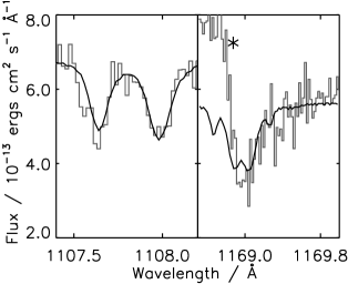
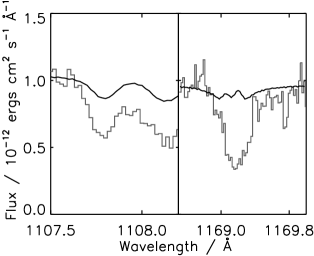
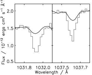
The results of the analysis are listed in Table 4, and a summary of which lines were detected in each spectrum is shown in Table 7. Heavy elements were detected in all objects studied. Carbon and nitrogen were identified in all objects, although the strength of the lines could not be reproduced with the abundances included in the models in some cases. Figure 2 shows an example of a fit to the carbon lines in the spectrum of LB 2, where the model successfully reproduced the strength of the lines in the real data. However, when a fit to the carbon lines in the spectrum of HS 0505+0112 was attempted, it was found that, when the values of temperature, gravity and helium abundance determined from FUSE data were used, the line strengths predicted by the model were far too weak compared to what is observed (Figure 3). Oxygen lines were found to be, in general, particularly difficult to fit, with no abundance measurement recorded in a number of cases because the reproduction of the lines was so poor. An example of a poor fit is shown in Figure 4. Silicon was also detected in all the spectra, but not iron. Nickel abundances were very poorly constrained, with many non-detections, although the error margins spanned the entire abundance range of the model grid in three cases.

Table 4: Measurements of abundances, with all values expressed as a number fraction with respect to hydrogen, and their 3$\sigma$ confidence intervals. Where the abundance value or the upper confidence boundary exceeded the highest abundance of the model grid, an $\infty$ symbol is used. Where an abundance or a lower error boundary is below the lowest abundance in the model grid, 0 is placed in the table; if this occurs for the abundance, the value in the +3$\sigma$ column is an upper limit on the abundance. In the table, * indicates that the model fit to the lines was poor, with $\chi^{2}_{red}$ greater than 2, while # is written instead of an abundance where the model was unable to recognisably reproduce the shape of the lines.

Object	C/H						N/H
	Optical			FUSE			Optical			FUSE
PN A66 7	1.38${}^{+}_{-}$	${}_{0.531}^{1.54}$ $\times$10	-5	4.17${}^{+}_{-}$	${}_{1.09}^{3.84}$ $\times$10	-5	7.96${}^{+}_{-}$	${}_{5.96}^{12.2}$ $\times$10	-8	6.43${}^{+}_{-}$	${}_{5.96}^{23.3}$ $\times$10	-6
H 0505+0112	1.11${}^{+}_{-}$	${}_{0.363}^{\infty}$ $\times$10	-4	$\infty$			7.36∗${}^{+}_{-}$	${}_{4.60}^{7.98}$ $\times$10	-8	$\infty$
PN PuWe 1	1.44∗${}^{+}_{-}$	${}_{0.975}^{2.22}$ $\times$10	-5	4.00∗${}^{+}_{-}$	${}_{1.74}^{5.08}$ $\times$10	-5	$\infty$			$\infty$
RE 0720-318	1.10${}^{+}_{-}$	${}_{0.563}^{0.728}$ $\times$10	-6	2.97${}^{+}_{-}$	${}_{1.45}^{1.90}$ $\times$10	-6	1.29${}^{+}_{-}$	${}_{0.714}^{0.778}$ $\times$10	-7	1.21${}^{+}_{-}$	${}_{0.467}^{0.689}$ $\times$10	-7
Ton 320	7.21${}^{+}_{-}$	${}_{3.01}^{4.73}$ $\times$10	-6	2.61${}^{+}_{-}$	${}_{1.39}^{2.63}$ $\times$10	-5	1.36${}^{+}_{-}$	${}_{1.13}^{2.13}$ $\times$10	-6	4.99${}^{+}_{-}$	${}_{0.0660}^{\infty}$ $\times$10	-5
PG 0834+500	2.91∗${}^{+}_{-}$	${}_{1.44}^{3.51}$ $\times$10	-6	6.93${}^{+}_{-}$	${}_{4.35}^{\infty}$ $\times$10	-5	6.89${}^{+}_{-}$	${}_{2.84}^{5.71}$ $\times$10	-6	$\infty$
PN A66 31	2.11${}^{+}_{-}$	${}_{1.41}^{2.10}$ $\times$10	-5	4.09${}^{+}_{-}$	${}_{1.52}^{5.50}$ $\times$10	-5	1.24${}^{+}_{-}$	${}_{0}^{14.9}$ $\times$10	-7	5.45${}^{+}_{-}$	${}_{0}^{50.2}$ $\times$10	-7
HS 1136+6646	1.83∗${}^{+}_{-}$	${}_{0.418}^{0.488}$ $\times$10	-6	3.19∗${}^{+}_{-}$	${}_{1.24}^{1.29}$ $\times$10	-5	6.67∗${}^{+}_{-}$	${}_{1.62}^{6.46}$ $\times$10	-7	$\infty$
Feige 55	2.84∗${}^{+}_{-}$	${}_{0.199}^{0.197}$ $\times$10	-6	5.01∗${}^{+}_{-}$	${}_{0.311}^{0.542}$ $\times$10	-6	2.11∗${}^{+}_{-}$	${}_{0.103}^{0.205}$ $\times$10	-6	$\infty$
PG 1210+533				4.30${}^{+}_{-}$	${}_{2.60}^{2.67}$ $\times$10	-6				1.50${}^{+}_{-}$	${}_{0.641}^{1.46}$ $\times$10	-6
LB 2	2.26${}^{+}_{-}$	${}_{1.22}^{1.17}$ $\times$10	-5	2.28${}^{+}_{-}$	${}_{1.27}^{3.05}$ $\times$10	-5	2.51∗${}^{+}_{-}$	${}_{0.864}^{1.40}$ $\times$10	-6	$\infty$
HZ 34	1.27${}^{+}_{-}$	${}_{0.563}^{3.56}$ $\times$10	-6	4.01${}^{+}_{-}$	${}_{1.43}^{9.51}$ $\times$10	-6	2.74${}^{+}_{-}$	${}_{2.59}^{12.7}$ $\times$10	-6	3.21${}^{+}_{-}$	${}_{3.08}^{\infty}$ $\times$10	-5
PN A66 39	1.66${}^{+}_{-}$	${}_{1.16}^{2.18}$ $\times$10	-6	1.66${}^{+}_{-}$	${}_{0.952}^{21.4}$ $\times$10	-6	5.60${}^{+}_{-}$	${}_{5.06}^{\infty}$ $\times$10	-6	4.08${}^{+}_{-}$	${}_{3.87}^{\infty}$ $\times$10	-5
RE 2013+400	1.61${}^{+}_{-}$	${}_{1.49}^{3.09}$ $\times$10	-6	1.61${}^{+}_{-}$	${}_{1.52}^{4.01}$ $\times$10	-6	8.36${}^{+}_{-}$	${}_{2.03}^{2.62}$ $\times$10	-7	3.01${}^{+}_{-}$	${}_{1.11}^{6.36}$ $\times$10	-6
PN DeHt 5				7.60${}^{+}_{-}$	${}_{7.20}^{96.6}$ $\times$10	-7				1.08${}^{+}_{-}$	${}_{0}^{\infty}$ $\times$10	-5
GD 561	1.16 ∗${}^{+}_{-}$	${}_{0.409}^{1.96}$ $\times$10	-5	9.19 ∗${}^{+}_{-}$	${}_{5.64}^{\infty}$ $\times$10	-5	$\infty$			$\infty$

Table 5: continued

Object

O/H

Si/H

Optical

FUSE

Optical

FUSE

PN A66 7

#

#

7.54∗${}^{+}_{-}$

${}_{3.97}^{3.57}$ $\times$10

-6

2.27∗${}^{+}_{-}$

${}_{1.08}^{1.04}$ $\times$10

-5

HS 0505+0112

#

#

1.67∗${}^{+}_{-}$

${}_{0.498}^{0.695}$ $\times$10

-6

7.71∗${}^{+}_{-}$

${}_{2.94}^{1.77}$ $\times$10

-5

PN PuWe 1

9.58∗${}^{+}_{-}$

${}_{6.54}^{6.10}$ $\times$10

-7

2.30∗${}^{+}_{-}$

${}_{2.06}^{1.19}$ $\times$10

-6

9.51∗${}^{+}_{-}$

${}_{6.55}^{10.1}$ $\times$10

-6

2.99∗${}^{+}_{-}$

${}_{2.09}^{1.11}$ $\times$10

-5

RE 0720-318

2.95${}^{+}_{-}$

${}_{1.38}^{1.12}$ $\times$10

-6

3.04${}^{+}_{-}$

${}_{0.877}^{3.18}$ $\times$10

-7

6.28${}^{+}_{-}$

${}_{1.26}^{2.47}$ $\times$10

-7

6.06${}^{+}_{-}$

${}_{1.45}^{1.17}$ $\times$10

-7

Ton 320

$\infty$

3.05∗${}^{+}_{-}$

${}_{1.09}^{0.0786}$ $\times$10

-6

4.33∗${}^{+}_{-}$

${}_{3.16}^{4.33}$ $\times$10

-7

3.73∗${}^{+}_{-}$

${}_{2.02}^{5.44}$ $\times$10

-6

PG 0834+500

$\infty$

5.67∗${}^{+}_{-}$

${}_{2.77}^{4.28}$ $\times$10

-7

2.81∗${}^{+}_{-}$

${}_{0.912}^{0.758}$ $\times$10

-6

3.00∗${}^{+}_{-}$

${}_{0.420}^{0.961}$ $\times$10

-5

PN A66 31

3.11∗${}^{+}_{-}$

${}_{0.798}^{2.76}$ $\times$10

-5

3.04∗${}^{+}_{-}$

${}_{0.902}^{0.649}$ $\times$10

-5

3.53∗${}^{+}_{-}$

${}_{1.51}^{2.71}$ $\times$10

-6

9.42∗${}^{+}_{-}$

${}_{2.42}^{4.33}$ $\times$10

-6

HS 1136+6646

4.76∗${}^{+}_{-}$

${}_{0.919}^{1.13}$ $\times$10

-5

9.60∗${}^{+}_{-}$

${}_{0.764}^{1.62}$ $\times$10

-7

4.40∗${}^{+}_{-}$

${}_{0}^{2.96}$ $\times$10

-8

1.32∗${}^{+}_{-}$

${}_{0.748}^{1.50}$ $\times$10

-6

Feige 55

1.03∗${}^{+}_{-}$

${}_{0.820}^{1.26}$ $\times$10

-5

3.80∗${}^{+}_{-}$

${}_{0.337}^{0.370}$ $\times$10

-7

5.52∗${}^{+}_{-}$

${}_{0.732}^{0.820}$ $\times$10

-7

5.15∗${}^{+}_{-}$

${}_{1.02}^{1.01}$ $\times$10

-6

PG 1210+533

2.99${}^{+}_{-}$

${}_{2.00}^{2.40}$ $\times$10

-6

1.90${}^{+}_{-}$

${}_{0.458}^{0.516}$ $\times$10

-8

LB 2

$\infty$

3.98∗${}^{+}_{-}$

${}_{1.11}^{2.97}$ $\times$10

-7

1.81${}^{+}_{-}$

${}_{0.587}^{0.730}$ $\times$10

-6

9.84${}^{+}_{-}$

${}_{3.53}^{6.69}$ $\times$10

-6

HZ 34

3.03 ∗${}^{+}_{-}$

${}_{0.606}^{0.362}$ $\times$10

-5

3.04∗${}^{+}_{-}$

${}_{1.19}^{0.209}$ $\times$10

-7

4.73${}^{+}_{-}$

${}_{2.41}^{3.76}$ $\times$10

-6

5.76${}^{+}_{-}$

${}_{2.74}^{20.9}$ $\times$10

-6

PN A66 39

#

#

2.33${}^{+}_{-}$

${}_{1.24}^{1.81}$ $\times$10

-6

3.00${}^{+}_{-}$

${}_{1.27}^{5.11}$ $\times$10

-6

RE 2013+400

#

#

3.68${}^{+}_{-}$

${}_{0.845}^{0.963}$ $\times$10

-7

4.71${}^{+}_{-}$

${}_{1.06}^{1.31}$ $\times$10

-7

PN DeHt 5

7.00${}^{+}_{-}$

${}_{1.92}^{13.0}$ $\times$10

-6

8.22${}^{+}_{-}$

${}_{4.10}^{11.8}$ $\times$10

-7

GD 561

2.64∗${}^{+}_{-}$

${}_{1.28}^{\infty}$ $\times$10

-4

#

5.24∗${}^{+}_{-}$

${}_{2.36}^{2.35}$ $\times$10

-6

9.51∗${}^{+}_{-}$

${}_{1.34}^{4.11}$ $\times$10

-6

Table 6: continued

Object	Fe/H						Ni/H
	Optical			FUSE			Optical			FUSE
PN A66 7	1.24∗${}^{+}_{-}$	${}_{0.744}^{1.17}$ $\times$10	-5	8.22∗${}^{+}_{-}$	${}_{3.82}^{7.25}$ $\times$10	-5	0${}^{+}_{-}$	${}_{0}^{1.63}$ $\times$10	-6	0${}^{+}_{-}$	${}_{0}^{8.94}$ $\times$10	-6
HS 0505+0112	8.77∗${}^{+}_{-}$	${}_{2.93}^{13.1}$ $\times$10	-5	9.68∗${}^{+}_{-}$	${}_{6.19}^{4.06}$ $\times$10	-5	1.53${}^{+}_{-}$	${}_{0}^{5.30}$ $\times$10	-6	0${}^{+}_{-}$	${}_{0}^{\infty}$
PN PuWe 1	2.96${}^{+}_{-}$	${}_{0}^{11.2}$ $\times$10	-6	3.40${}^{+}_{-}$	${}_{0}^{16.4}$ $\times$10	-6	1.23${}^{+}_{-}$	${}_{0}^{31.4}$ $\times$10	-6	5.65${}^{+}_{-}$	${}_{0}^{\infty}$ $\times$10	-6
RE 0720-318	1.32${}^{+}_{-}$	${}_{0}^{6.62}$ $\times$10	-6	2.44${}^{+}_{-}$	${}_{0}^{13.3}$ $\times$10	-6	3.45${}^{+}_{-}$	${}_{0}^{46.1}$ $\times$10	-7	7.21${}^{+}_{-}$	${}_{0}^{102.}$ $\times$10	-7
Ton 320	1.70∗${}^{+}_{-}$	${}_{1.16}^{2.37}$ $\times$10	-5	8.73∗${}^{+}_{-}$	${}_{4.64}^{16.3}$ $\times$10	-5	5.43${}^{+}_{-}$	${}_{0}^{65.1}$ $\times$10	-7	1.82${}^{+}_{-}$	${}_{0}^{29.7}$ $\times$10	-6
PG 0834+500	1.82∗${}^{+}_{-}$	${}_{0.926}^{3.18}$ $\times$10	-5	4.75∗${}^{+}_{-}$	${}_{3.42}^{4.17}$ $\times$10	-4	8.41${}^{+}_{-}$	${}_{0}^{42.5}$ $\times$10	-6	2.21${}^{+}_{-}$	${}_{0}^{\infty}$ $\times$10	-5
PN A66 31	9.42∗${}^{+}_{-}$	${}_{5.52}^{8.36}$ $\times$10	-5	3.16∗${}^{+}_{-}$	${}_{1.52}^{2.20}$ $\times$10	-4	2.22${}^{+}_{-}$	${}_{0}^{39.5}$ $\times$10	-7	7.36${}^{+}_{-}$	${}_{0}^{234.}$ $\times$10	-7
HS 1136+6646	5.38∗${}^{+}_{-}$	${}_{0}^{11.5}$ $\times$10	-6	0∗${}^{+}_{-}$	${}_{0}^{2.31}$ $\times$10	-6	0∗${}^{+}_{-}$	${}_{0}^{5.89}$ $\times$10	-7	0∗${}^{+}_{-}$	${}_{0}^{2.48}$ $\times$10	-5
Feige 55	1.40∗${}^{+}_{-}$	${}_{0.439}^{0.616}$ $\times$10	-5	1.41∗${}^{+}_{-}$	${}_{0.358}^{0.480}$ $\times$10	-5	5.55${}^{+}_{-}$	${}_{3.73}^{8.54}$ $\times$10	-6	3.71${}^{+}_{-}$	${}_{2.21}^{6.22}$ $\times$10	-6
PG 1210+533				4.70∗${}^{+}_{-}$	${}_{0}^{60.1}$ $\times$10	-6				3.29∗${}^{+}_{-}$	${}_{0}^{19.2}$ $\times$10	-6
LB 2	1.73∗${}^{+}_{-}$	${}_{1.10}^{1.92}$ $\times$10	-5	2.09${}^{+}_{-}$	${}_{1.06}^{2.42}$ $\times$10	-5	0${}^{+}_{-}$	${}_{0}^{3.12}$ $\times$10	-6	0${}^{+}_{-}$	${}_{0}^{7.37}$ $\times$10	-6
HZ 34	2.42${}^{+}_{-}$	${}_{1.68}^{5.82}$ $\times$10	-5	7.64${}^{+}_{-}$	${}_{5.91}^{51.0}$ $\times$10	-5	0${}^{+}_{-}$	${}_{0}^{6.63}$ $\times$10	-6	5.12${}^{+}_{-}$	${}_{0}^{1920.}$ $\times$10	-8
PN A66 39	4.89${}^{+}_{-}$	${}_{0}^{21.4}$ $\times$10	-6	3.74${}^{+}_{-}$	${}_{0}^{15.3}$ $\times$10	-6	4.37${}^{+}_{-}$	${}_{0}^{25.4}$ $\times$10	-6	9.93${}^{+}_{-}$	${}_{0}^{88.7}$ $\times$10	-6
RE 2013+400	0${}^{+}_{-}$	${}_{0}^{2.83}$ $\times$10	-5	0${}^{+}_{-}$	${}_{0}^{2.16}$ $\times$10	-5	0${}^{+}_{-}$	${}_{0}^{2.93}$ $\times$10	-5	0${}^{+}_{-}$	${}_{0}^{3.11}$ $\times$10	-5
PN DeHt 5				3.34${}^{+}_{-}$	${}_{2.58}^{6.20}$ $\times$10	-5				1.21${}^{+}_{-}$	${}_{1.19}^{7.27}$ $\times$10	-5
GD 561	1.55${}^{+}_{-}$	${}_{0.967}^{1.76}$ $\times$10	-5	1.45${}^{+}_{-}$	${}_{0.828}^{0.143}$ $\times$10	-5	1.84${}^{+}_{-}$	${}_{0}^{11.2}$ $\times$10	-6	1.78${}^{+}_{-}$	${}_{0}^{28.1}$ $\times$10	-6

Table 7: Summary of which lines were observed to be present when performing the abundance fits. H₂ denotes where lines were obscured by molecular hydrogen absorption.

Object	C iv	N iii	N iv	O iv	O vi	Si iii	Si iv	Fe v	Fe vi	FE vii	Ni v
PN A66 7	$\surd$	H2	$\surd$	$\surd$	$\surd$		$\surd$		$\surd$	$\surd$
HS 0505+0112	$\surd$	$\surd$	$\surd$	$\surd$	$\surd$		$\surd$			$\surd$
PN PuWe 1	$\surd$	H2	$\surd$	$\surd$	$\surd$		$\surd$
RE 0720-318	$\surd$	$\surd$	$\surd$		$\surd$	$\surd$	$\surd$
TON 320	$\surd$		$\surd$	$\surd$	$\surd$		$\surd$		$\surd$	$\surd$
PG 0834+500	$\surd$		$\surd$	$\surd$	$\surd$	$\surd$	$\surd$	$\surd$	$\surd$	$\surd$
PN A66 31	$\surd$	H2	$\surd$	$\surd$	$\surd$		$\surd$		$\surd$	$\surd$
HS 1136+6646	$\surd$		$\surd$	$\surd$	$\surd$		$\surd$
Feige 55	$\surd$	$\surd$	$\surd$	$\surd$	$\surd$		$\surd$	$\surd$	$\surd$		$\surd$
PG 1210+533	$\surd$	$\surd$	$\surd$	$\surd$	$\surd$	$\surd$	$\surd$
LB 2	$\surd$		$\surd$	$\surd$	$\surd$	$\surd$	$\surd$		$\surd$
HZ 34	$\surd$		$\surd$	$\surd$	$\surd$		$\surd$		$\surd$	$\surd$
PN A66 39	$\surd$	H2	$\surd$		$\surd$		$\surd$
RE 2013+400	$\surd$	$\surd$	$\surd$		$\surd$	$\surd$	$\surd$
PN DeHt 5	$\surd$	H2	$\surd$	$\surd$		$\surd$	$\surd$
GD 561	$\surd$	H2	$\surd$	$\surd$	$\surd$		$\surd$		$\surd$	$\surd$

Figure 2: The C iv lines observed in the spectrum of LB 2 (grey histogram), overlaid with the best fitting model (black line). The temperature, gravity and helium abundance of the model were those measured from FUSE data. * Bins containing the high fluxes that can be seen on the blue side of the right panel and that are not predicted by the model were excluded from the fit.

Figure 3: The C iv lines observed in the spectrum of HS 0505+0112 (grey histogram), overlaid with the best fitting model (black line). The temperature, gravity and helium abundance of the model were those measured from FUSE data. The heavy element abundance of the model is the maximum possible for the model grid used in the fit, yet the predicted lines are much weaker than those observed.

Figure 4: The O vi lines observed in the spectrum of RE 2013+400 (grey histogram), overlaid with a model that has an oxygen abundance of 10 times the values measured for G 191-B2B, and which uses the temperature, gravity and helium abundance measured from FUSE data (black line). The lines in the model are much weaker than those seen in the real data, no matter what abundance is chosen, and hence no oxygen abundance was recorded for this object.

The sample of DAOs and the sample of DAs of Barstow et al. (2003) contain one object in common: PN DeHt 5. Although this white dwarf does not have an observable helium line in its optical spectrum, it is included within the sample of DAOs because Barstow et al. (2001) detected helium within the Hubble Space Telescope (HST) Space Telescope Imaging Spectrometer (STIS) spectrum of the object. This presents an opportunity to compare the results of this work with the abundances measured by Barstow et al. (2003) to confirm the consistency of the measurements made in the different wavebands; this comparison is shown in Figure 5, and demonstrates that agreement between the sets of results is within errors. However, uncertainties in the measurements are large, particularly for nitrogen measured in this work.

Figure 5: Comparison of abundance measurements for DeHt 5 between Barstow et al. (2003) and this work. Note that Barstow et al. (2003) obtained abundances for C III and C IV separately. These are both compared to the carbon abundance determined in this work from fits to C iv lines.

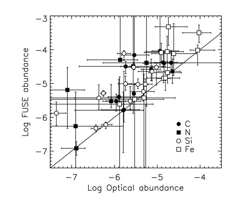
The abundances measured with the models that use the FUSE and optical measurements of temperature, gravity and helium abundance can also be compared from the results of this work. Changing the parameters of the model will affect its temperature structure and ionisation balance, and therefore the abundances measured may also change. The carbon, nitrogen, silicon and iron abundances measured using the FUSE derived parameters are compared to those measured using the optically derived parameters in Figure 6. Oxygen abundances are not shown due to the poor quality of the fits, while many of the nickel abundances are poorly constrained and hence are also not shown. The abundances that were measured with models that used the FUSE parameters are generally higher than those that used the optical parameters by a factor of between 1 and 10. In some cases the factor is higher, for example it is 30 for the silicon measurements for HS 1136+6646. However, a satisfactory fit to those lines was not achieved ($\chi^{2}_{red}>2$), hence the abundances may be unreliable. In contrast, the fits to the nitrogen lines in the spectrum of A 7 were satisfactory, yet the abundance measure that used the FUSE parameters was higher than the measure with optical parameters by a factor of 81, although the error bars are large. Overall, however, the abundance measures that utilise the different parameters appear to correlate with each other.

Figure 6: Comparison of the abundances of carbon, nitrogen, silicon and iron measured when the temperature, gravity and helium abundance derived from FUSE and optical data were used. Also shown is a line marking where the abundances are equal.

In the following we describe the abundance measurements for each element in turn, compare them to the DA measurements made by Barstow et al. (2003) and discuss them with reference to the radiative levitation predictions of Chayer, Fontaine, & Wesemael (1995), and the mass loss calculations of Unglaub & Bues (2000).

5.1 Carbon abundances

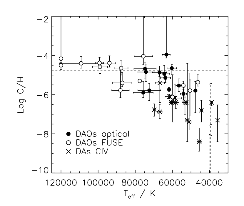
Figure 7 shows the measured carbon abundances against $T_{\mathrm{eff}}$from fits to the carbon absorption features in the FUSE data. Abundances obtained when the model $T_{\mathrm{eff}}$, log $g$ and helium abundance were set to the values found by Good et al. (2004) from fits to both optical and FUSE spectra are shown. In the following, these will be referred to as ‘optical abundances’ and ‘FUSE abundances’ respectively. Shown for comparison are the measurements made by Barstow et al. (2003) for DAs. For clarity, only the result of their fits to the C iv lines are plotted. The plot shows that the carbon abundances of the DAOs fall within the range 10^-6 to 10^-4 that of hydrogen, in general higher than those for the DAs. The only abundance below 10^-6 belongs to PN DeHt 5, which, apart from the discovery of helium in its HST spectrum by Barstow et al. (2001), would not be classed as a DAO in this work. The other DAO white dwarfs whose temperatures are similar to those of the DAs have marginally higher abundances than the latter. These DAOs comprise the white dwarf plus main sequence star binaries, the unusual white dwarf PG 1210+533, and optical abundances of stars whose $T_{\mathrm{eff}}$, as measured from FUSE data, were extreme (see Good et al., 2004). However, the highest abundance measured was for HS 0505+0112, which is also one of the extreme FUSE $T_{\mathrm{eff}}$ objects, for which the FUSE abundance and the upper limit of the optical abundance exceeded the upper limit of the model grid.

The predictions of Chayer, Fontaine, & Wesemael (1995) suggest that above $\sim$40 000 K, carbon abundances should have little dependence on temperature, but should increase with decreasing gravity. Taking the optical abundances together with the DA abundances, it might be argued that they form a trend of increasing temperature with gravity, extending to $\sim$80 000 K. Since the measurements of $T_{\mathrm{eff}}$ from FUSE were higher than those from optical data, the FUSE abundances are more spread out towards the higher temperatures than the optical abundances. The FUSE abundances do not show any trend with temperature, although the lower temperature objects and three others do have slightly lower abundances than the remainder; if the latter objects (Feige 55, HZ 34 and PN A 39) had high log $g$, this might explain their low carbon abundances, but this does not seem to be the case. Overall, no carbon abundance was greater than $\sim$10^-4 that of hydrogen, which is quite close to the maximum abundance predicted by Chayer, Fontaine, & Wesemael (1995), illustrated in Figure 7 by the dashed line. However the carbon abundances decrease below $\sim$80 000 K, contrary to their predictions. Unglaub & Bues (2000) predict a surface abundance of carbon of between 10^-3 and 10^-4 times the number of heavy particles in their simulation. Their calculations end at their wind limit, when the wind is expected to cease, at approximately 90 000 K. After this point, Unglaub & Bues (2000) expect the abundances to fall to the values expected when there is equilibrium between gravitational settling and radiative acceleration. When using an alternative prescription for mass loss, which does not have a wind limit, the drop off occurs at lower temperature, at approximately 80 000 K. This is similar to what is observed, although the abundance measurements are a factor $\sim$10 smaller than predicted.

Figure 7: Carbon abundances measured for the DAOs against $T_{\mathrm{eff}}$, when the temperature, gravity and helium abundance were fixed according to the values measured by Good et al. (2004) from fits to hydrogen Balmer lines (filled circles) and hydrogen Lyman lines (open circles). Also shown for comparison are the results of Barstow et al. (2003) for DA white dwarfs (crosses). The dashed arrows mark the 3$\sigma$ upper abundance limit for the DAs, where carbon was not detected. The approximate position of the abundances predicted by Chayer, Fontaine, & Wesemael (1995) for a DA white dwarf with a log $g$ of 7.0 is shown as a dashed line.

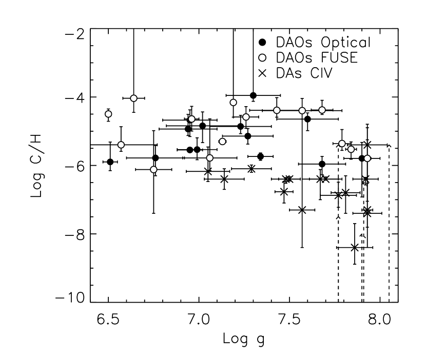
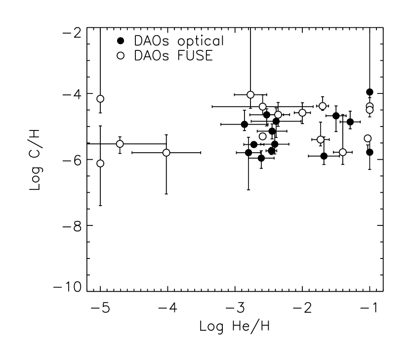
The dependence of carbon abundance on gravity is shown in Figure 8. Good et al. (2004) found no systematic differences between log $g$ measured from optical and FUSE data, hence there is no separation between the optical and FUSE abundances, as seen in Figure 7. No trend between log $g$ and carbon abundance is evident, in contrast to what might be expected from the results of Chayer, Fontaine, & Wesemael (1995). Figure 9 shows the relationship between carbon and helium abundance. As with Figure 8, no trend is evident. Four of the points are separated from the rest because of their low helium abundance measured from optical data; this is discussed in Good et al. (2004) and does not appear to be reflected in the carbon abundance.

Figure 8: Carbon abundances measured for the DAOs against log $g$, when the temperature, gravity and helium abundance were fixed according to the values measured by Good et al. (2004) from fits to hydrogen Balmer lines (filled circles) and hydrogen Lyman lines (open circles). Also shown for comparison are the results of Barstow et al. (2003) for DA white dwarfs (crosses). The dashed arrows mark the 3$\sigma$ upper abundance limit for the DAs, where carbon was not detected.

Figure 9: Carbon abundances measured for the DAOs against log $\frac{He}{H}$, when the temperature, gravity and helium abundance were fixed according to the values measured by Good et al. (2004) from fits to hydrogen Balmer lines (filled circles) and hydrogen Lyman lines (open circles).

5.2 Nitrogen abundances

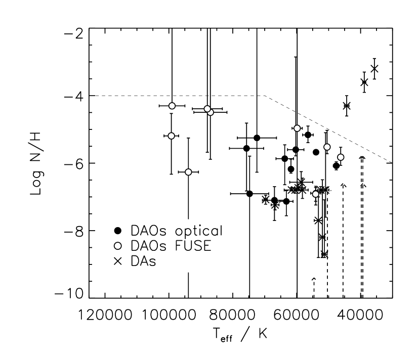
Figure 10 shows the nitrogen abundance measurements, plotted against effective temperature. A number of the abundances are relatively poorly constrained, and exceed the upper bound of the model grid. In contrast, the lower 3$\sigma$ error bounds for PN A 31 and PN DeHt 5 both reach below the lowest abundance in the model grid, with, in the latter case, the error bounds extending across the whole range of the model grid. There is no obvious trend between $T_{\mathrm{eff}}$ and either the optical or FUSE abundances, in contrast to the predictions of Chayer, Fontaine, & Wesemael (1995) and Unglaub & Bues (2000), although the abundances are close to those predicted from radiative levitation theory. None of the lower temperature DAOs have the comparatively high abundances found for three of the DAs of Barstow et al. (2003). As with carbon, the DAO nitrogen abundances are often higher than those of the DAs. However, the lower temperature DAOs do not, in general, have nitrogen abundances different from the higher temperature objects, despite the possible differences in their evolutionary paths. RE 0720-318 has a nitrogen abundance similar to the DAs, and less than most of the DAOs, according to the abundances determinations using both the optical and FUSE parameters. Three other objects (PN A 7, HS 0505+0112 and PN A 31) have comparatively low abundances when the optically determined parameters were used. However, this was not the case when the FUSE parameters were used.

Figure 10: As Figure 7, but showing nitrogen abundances.

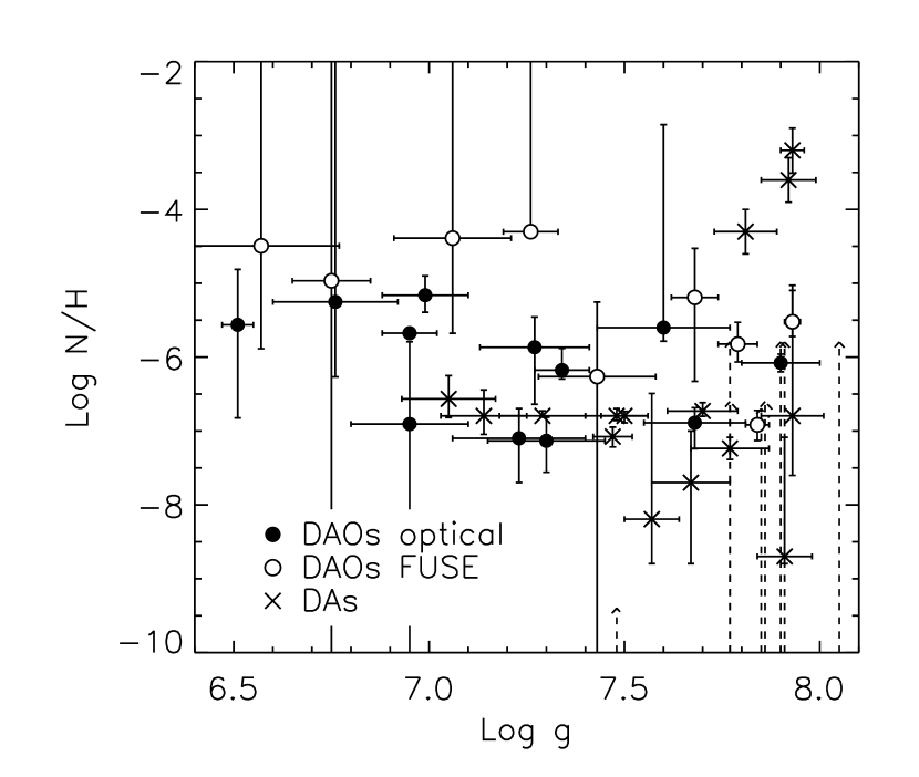
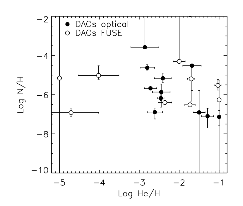
In Figures 11 and 12, nitrogen abundances are plotted against log $g$ and log $\frac{He}{H}$. As for carbon, no trend with gravity or helium abundance is evident.

Figure 11: As Figure 8, but showing nitrogen abundances.

Figure 12: As Figure 9, but showing nitrogen abundances.

5.3 Oxygen abundances

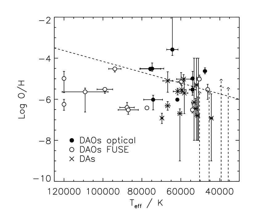
All the DAOs were found to have evidence of oxygen absorption in their spectra. This absorption is believed to originate in the white dwarf as the radial velocity of the lines are not consistent with those of interstellar absorption features. The DAO oxygen abundances, shown in Figure 13 against $T_{\mathrm{eff}}$, are very similar to those of the DAs and show no obvious dependence on temperature. Again, the lower temperature DAOs do not appear to have abundances different from the higher temperature objects. However, the reproduction of the observed oxygen lines by the models was very poor, with the problem affecting both high and low temperature DAOs. For only three objects, RE 0720-318, PG 1210+533 and PN DeHt 5, was a fit with an acceptable value of $\chi^{2}_{red}$ ($<$ 2) achieved. In general the lines predicted by the models were too weak compared to the observed lines. In four cases an abundance was not even recorded for either optical or FUSE abundances, and in one case (GD 561) for the FUSE abundance alone, due to the disagreement between the model and data (see, for example, Figure 4). The poor quality of the fits means that the results are probably not reliable, and we do not show plots of abundance against gravity or helium abundance.

Figure 13: As Figure 7, but showing oxygen abundances.

5.4 Silicon abundances

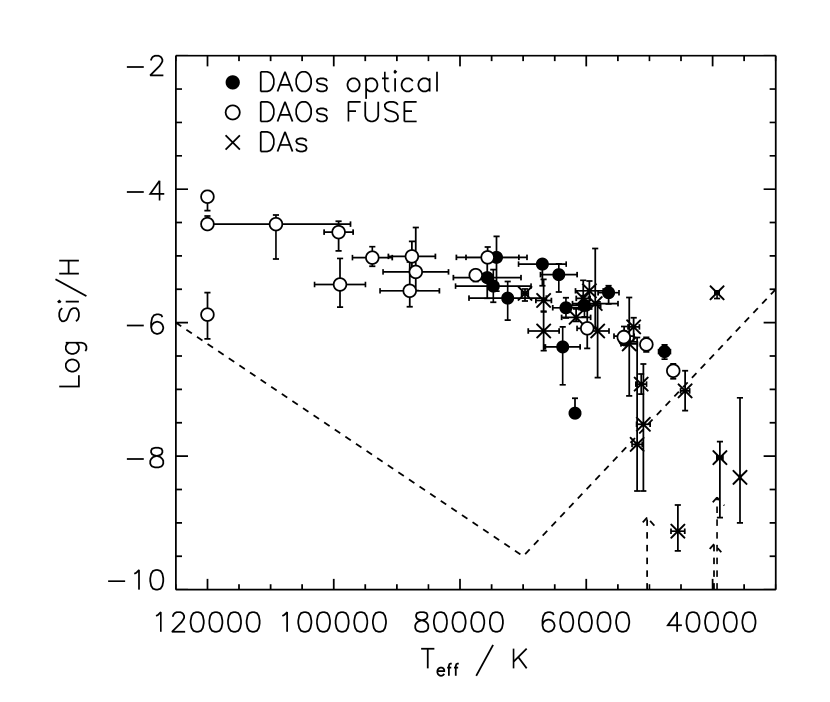
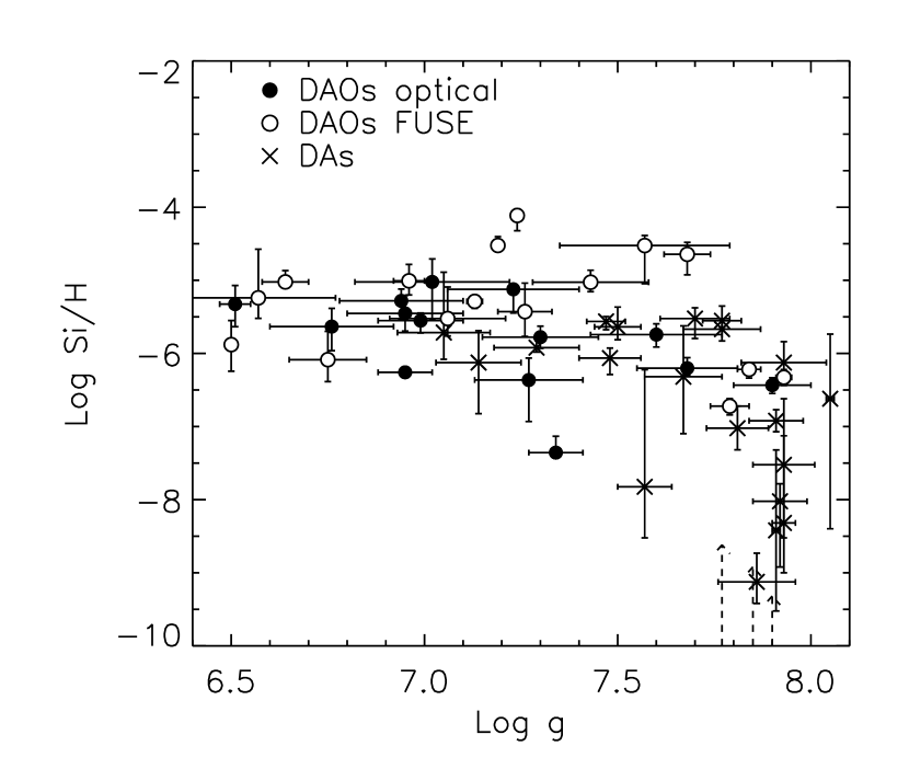
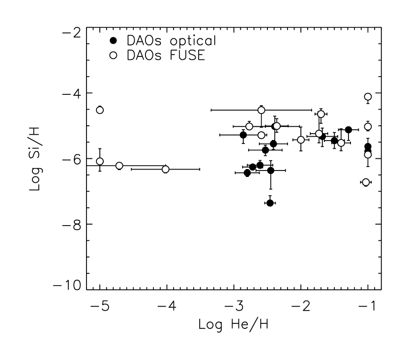
Figure 14 shows the measured silicon abundances against $T_{\mathrm{eff}}$. The optical abundances, when considered along with the DA abundances, appear to show an increase with temperature. The FUSE abundances also show a slight increase with temperature, with the maximum abundance observed $\sim$10^-4 that of hydrogen. The calculations of Chayer, Fontaine, & Wesemael (1995) predict a minimum at 70 000 K, which is not observed here, although Barstow et al. (2003) did note an apparent minimum at $\sim$40 000 K in the DA abundances. However, as with the oxygen measurements, the fits were often poor and in approximately half the cases $\chi^{2}_{red}<$ 2 was not achieved. The abundance measurements for HS 1136+6646 are lower than for the other DAOs. This is one of the objects for which satisfactory fits were not achieved; it is also one of the DAOs with extreme $T_{\mathrm{eff}}$, as measured from FUSE data. In Figure 15, we plot the silicon abundances against log $g$. Similarly, Figure 16 shows the relationship between heavy element abundances and helium abundances. In neither are any strong trends evident.

Figure 14: As Figure 7, but showing silicon abundances.

Figure 15: As Figure 8, but showing silicon abundances.

Figure 16: As Figure 9, but showing silicon abundances.

5.5 Iron abundances

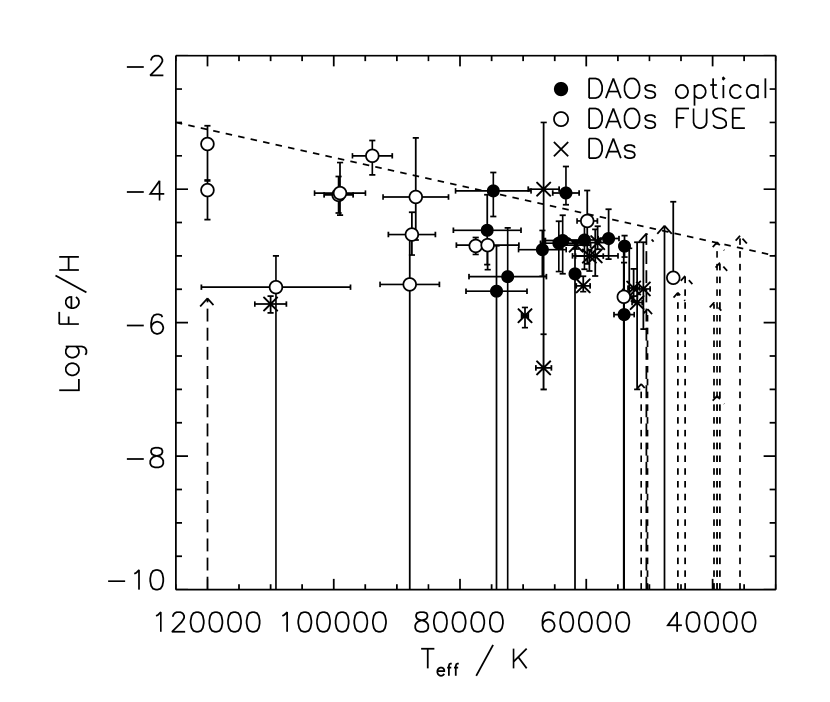
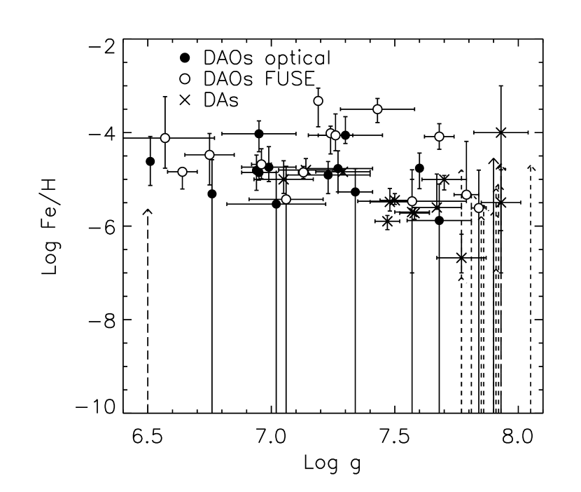
Fits to the iron lines were unsatifactory for, again, approximately half the objects. Apart from three, these were the same objects for which the fits to the silicon lines were also poor. Included in these are the three objects with extreme FUSE-measured $T_{\mathrm{eff}}$, and also PG 1210+533, which has a temperature and gravity that would be considered normal for a DA white dwarf. Iron was not predicted in the spectrum of RE 2013+400, nor that of HS 1136+6646 when the FUSE-derived values of $T_{\mathrm{eff}}$, log $g$ and helium abundance were used. The lower error boundary reached beyond the lowest abundance in the model grid in eleven cases. Figure 17 illustrates the relationship between iron abundance and $T_{\mathrm{eff}}$. This demonstrates that the optical and FUSE abundances measured for iron are similar to those measured in the DAs, where iron was detected at all. There is no strong indication of an increase in the abundances with temperature as might be expected from radiative levitation theory. However, the measured abundances are quite close to the predictions. No strong differences between the iron abundances of lower and higher temperature DAOs is evident. Similarly, Figure 18 shows no increase in abundance with decreasing gravity as might also be expected. Finally, there are also no trends evident in the plot of iron abundances against helium abundances (Figure 19).

Figure 17: As Figure 7, but showing iron abundances. Solid and long dashed arrows mark the 3$\sigma$ upper limits for the optical and FUSE abundances, respectively, where iron was not detected.

Figure 18: As Figure 8, but showing iron abundances. Solid and long dashed arrows mark the 3$\sigma$ upper limits for the optical and FUSE abundances, respectively, where iron was not detected.

Figure 19: As Figure 9, but showing iron abundances. Solid and long dashed arrows mark the 3$\sigma$ upper limits for the optical and FUSE abundances, respectively, where iron was not detected.

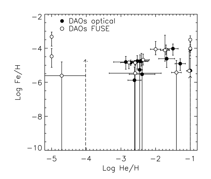
5.6 Nickel abundances

The nickel lines in the FUSE wavelength range that were used for abundance measurements were weak, hence the results were poorly constrained. There were a number of non-detections, and the lower bounds for all but three of the measurements were below the range of the model grid. In addition, three had upper bounds above the highest abundance in the grid and thus their error bars span the entire range of the models. In no cases was the measured abundance above $\log\frac{Ni}{H}>-4$, and no trends are evident.

5.7 Iron/nickel ratio

Barstow et al. (2003) found the ratio between the iron and nickel abundances for the DAs to be approximately constant, at the solar value of $\sim$20, rather than the prediction of Chayer et al. (1994) of close to unity. For the DAOs, approximately half have Fe/Ni ratio between 1 and 20, and all but two of the remainder have ratios greater than 20. However these ratios are very poorly constrained by the fits to FUSE data, thus preventing definite conclusions about the iron/nickel ratio in DAO white dwarfs.

6 Discussion

The investigation of heavy element abundances in DAO white dwarfs has provided an opportunity to investigate the ability of our homogeneous models to reproduce the observed lines, when temperatures derived from optical and FUSE data were used. These are observed to differ greatly in some cases; Table 8 lists those objects for which temperature disagreements were noted by Good et al. (2004).

Table 8: A list of objects whose optical and FUSE temperatures agree and those that disagree, separated into those where an empirical relationship between the two can be found, and those with FUSE temperatures greater than 120 000 K.

Agree	Disagree
	FUSE $T_{\mathrm{eff}}$
	$<$120,000 K	$>$120,000 K
RE 0720-318	PN A66 7	HS 0505+0112
PG 1210+533	PN PuWe 1	PG 0834+500
RE 2013+400	Ton 320	HS 1136+6646
PN DeHt 5	PN A66 31
	Feige 55
	LB 2
	HZ 34
	PN A66 39
	GD 561

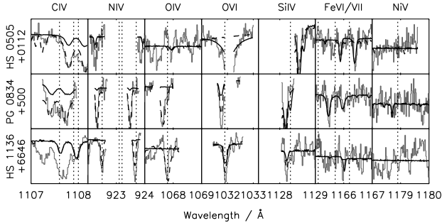
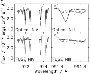
In §5, it was found that when the FUSE values of temperature, gravity and helium abundance were used, the abundances tended to be between a factor 1 and 10 greater than those where the optical values are utilised. Inspection of Table 4 shows that abundances of heavy elements, or their upper limits, exceeded the quantities within the model grid more often in the FUSE results, for example for the carbon measurement of HS 0505+0112, which is one of the extreme temperature objects. Satisfactory fits ($\chi^{2}_{red}<$ 2) were achieved in approximately equal number when the two sets of parameters were used. Figure 20 shows examples of fits to the spectra of objects where the optical and FUSE temperatures agree closely. As might be expected, little difference is seen between the ability of the models that use the optical and FUSE parameters to reproduce the data. For the objects where there are differences between the optical and FUSE temperatures (Figure 21), large differences are seen between the reproduction of the oxygen lines. The models that use the comparatively high FUSE temperatures do not have strong O iv lines. However, the models that use the optical temperatures are able to reproduce the lines. The O vi lines are not well reproduced by the models, except in a few cases, for example GD 561. In contrast, the iron lines tend to be better reproduced by the models that use the FUSE data, as the lines predicted by the model with optical parameters are too weak. In addition, Figure 22 compares the strengths of N iii and N iv lines in the spectrum of LB 2 when the optical and FUSE parameters were adopted. Although in neither case was the N iii line well reproduced, the model that uses the FUSE parameters is closer to what is observed.

Figure 20: Comparisons of the strengths of lines in the data (grey histograms) to those predicted by the models when the optical (dashed lines) and FUSE (solid lines) parameters were used, for those objects where the optical and FUSE temperatures agree. The vertical axis is scaled individually for each panel to encompass the range of fluxes in that region of the spectrum. Vertical dashed lines indicate the laboratory wavelength of the lines predicted by the models. Additional lines seen in some panels (for example PN DeHt 5 C iv and Ovi) are due to molecular hydrogen absorption. Regions of the spectra containing other photospheric lines, unexplained emission, or where the molecular hydrogen model did not adequately reproduce the shape of the lines, were removed to avoid them influencing the fits.

Figure 21: As Figure 20 for those objects where the optical and FUSE temperatures do not agree.

Figure 22: Comparisons of line strengths predicted by the models (black line) to the data (grey histogram) for N iii and N iv lines in the spectrum of LB 2, when $T_{\mathrm{eff}}$, log $g$ and log $\frac{He}{H}$ determined from Balmer and Lyman line analyses are used.

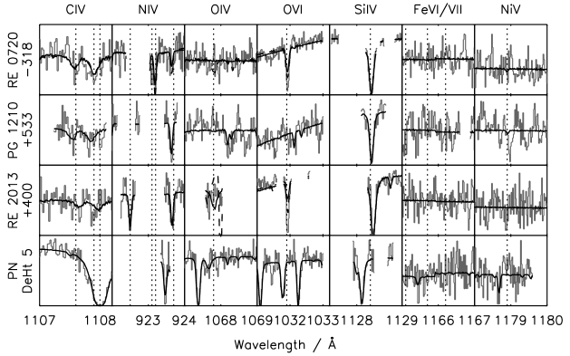
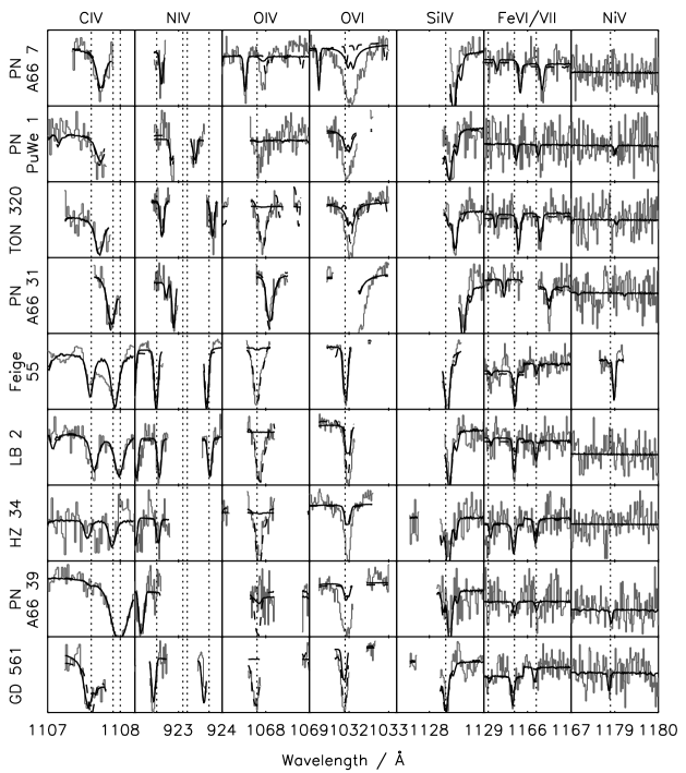
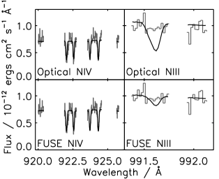
Figure 23 show example fits for the objects where the FUSE measure of temperature exceeded 120 000 K. Due to the extreme temperature, the C iv, N iv and O iv lines are predicted to be too weak by the models that use the FUSE temperature. However, when looking in detail at the nitrogen lines in the spectrum of HS 1136+6646 (Figure 24), it is evident that neither model is able to reproduce the lines, with the N iii line in the model that uses the optical parameters too strong, and the N iv lines in the FUSE parameters model too weak.

Figure 23: As Figure 20 for those objects where the FUSE temperature exceeded 120 000 K.

Figure 24: Comparisons of line strengths predicted by the models (black line) to the data (grey histogram) for N iii and N iv lines in the spectrum of HS 1136+6646, when $T_{\mathrm{eff}}$, log $g$ and log $\frac{He}{H}$ determined from Balmer and Lyman line analyses are used.

It is therefore evident that the models that use the optical parameter better reproduce the oxygen features than models that use the FUSE data, while the reverse is true for other lines such as nitrogen and iron. These differences between the models and data could be caused by a number of effects. It is not known if either the optical or FUSE stellar parameters are correct. Therefore, if both are wrong the ability of the models to reproduce the data might be influenced by the use of the incorrect parameters. However, this points to the underlying problem of why the optical and FUSE parameters are different, and if this problem could also affect the strength of the lines in the models. A possibility for the cause of these differences is the assumption of chemical homogeneity in the models. Evidence of stratification of heavy elements in white dwarf atmospheres have been found by other authors (e.g. Barstow, Hubeny, & Holberg, 1999), and this can have a strong affect on the predicted line strengths. For example O vi lines, which do not appear in homogeneous models below $\sim$50 000 K, can be prominent at lower temperatures when a stratified model is used (Chayer et al., 2003). With the development of stratified models (e.g. Schuh, Dreizler, & Wolff, 2002), these differences might be resolved, although the assumptions made within those particular models are probably not appropriate to DAO white dwarfs, because of the processes such as mass loss that are thought to be occurring.

A further cause of discrepancies between the data and models may be due to the limitations of the fitting process. During the fitting procedure, the abundance of all the elements are varied by the same factor. Therefore, the abundance of one element is measured with a model that contains the same relative abundance of all the other elements, even if those elements are not present in that particular object, or are present in different amounts. This may alter the temperature structure of the model, changing the line strengths. Ideally, models would be calculated for a range of abundances of every element and a simultaneous fit of all the absorption lines performed. Such an approach may be possible in the future with increases in computing power.

In conclusion, there is disagreement between the predictions of the homogeneous models used in this work and the observed line strengths of different ionisation states when both the optical and FUSE stellar parameters are used. Therefore, it is not possible to draw strong conclusions from these results to say which of the optical and FUSE measurements of $T_{\mathrm{eff}}$ are more likely to be correct.

7 Conclusions

Abundance measurements of heavy elements in the atmospheres of DAO white dwarfs have been performed using FUSE data. All the DAOs in our sample were found to contain heavy element absorption lines. Two sets of metal abundances were determined using stellar parameters ($T_{\mathrm{eff}}$, log $g$ and $\log\frac{He}{H}$) determined from both FUSE and optical data. The results were compared to a similar analysis for DAs conducted by Barstow et al. (2003), to the predictions for radiative levitation made by Chayer, Fontaine, & Wesemael (1995), and the mass loss calculations of Unglaub & Bues (2000). For carbon, the DAOs were found, in general, to have higher abundances than those measured for the DAs. When considered along with the DA abundances, the optical abundance measurements might be argued to form a trend of increasing abundance with temperature. However, this trend extends to a higher temperature than predicted by Chayer, Fontaine, & Wesemael (1995). The FUSE determined abundances do not follow this trend due to the higher temperatures determined from FUSE data. These abundance measurements do not increase with temperature, with no carbon abundance exceeding $10^{-4}$ that of hydrogen, which is close to the prediction of Chayer, Fontaine, & Wesemael (1995). The nitrogen abundances were poorly constrained for a number of the objects, and there was no obvious trend with temperature. Although oxygen lines were identified in all the spectra, fits to those lines were, in general, very poor, making the abundances unreliable. Silicon abundances were found to increase with temperature up to a maximum of $\sim$10^-4 that of hydrogen, and do not show a minimum at 70 000 K, as predicted by Chayer, Fontaine, & Wesemael (1995). However, approximately half the fits were of poor quality, as defined by $\chi^{2}_{red}>$2. Iron abundances were similar to those measured for DAs by Barstow et al. (2003) and no trend with temperature was seen. As with silicon, approximately half the fits were poor quality. Nickel abundances were poorly constrained with a number of non-detections, and no trends with temperature were evident. For none of the elements were trends with gravity or helium abundance found.

In general, it was found that the abundances measurements that used the parameters determined from FUSE data were higher than those that used the optically derived parameters by factors between 1-10. Satisfactory fits were achieved in approximately equal number for the optical and FUSE abundance measurements. The ability of the models to reproduce the observed line strengths was slightly better for the models that used the optically derived $T_{\mathrm{eff}}$, log $g$ and $\log\frac{He}{H}$ for oxygen and for the carbon, nitrogen and oxygen lines of those objects with FUSE temperature greater than 120 000 K. However, the reverse is true for the iron lines. For the example of the relative strength of N iii and N iv lines in the spectrum of one of the objects for which the optical and FUSE temperatures differ, the model with the FUSE temperature was better. However, for one of the objects with extreme FUSE temperatures, neither model was successful at reproducing the lines. The failure of the models to reproduce the line strengths might be caused by the assumption of chemical homogeneity. The use of stratified models, such as those developed by Schuh, Dreizler, & Wolff (2002) might help to resolve the discrepancies. In addition, the inability of the models to reproduce the lines might be influenced by the fitting technique used, in which the abundance of all elements were varied together. In the ideal case, the abundance of all elements would be measured simultaneously.

Overall, none of the measured abundances exeeded the expected levels significantly, except for silicon. For none of the elements, except silicon, were the abundances for the lower temperature DAOs significantly different to those for the hotter stars, despite the different evolutionary paths through which they are thought to evolve. The abundances were also not markedly different from the abundance measurements for the DAs, apart from what might be explained by the higher temperatures.

References

- Arnaud (1996) Arnaud K. A., 1996, ADASS, 5, 17
- Barstow et al. (2001) Barstow M. A., Bannister N. P., Holberg J. B., Hubeny I., Bruhweiler F. C., Napiwotzki R., 2001, MNRAS, 325, 1149
- Barstow et al. (2003) Barstow M. A., Good S. A., Burleigh M. R., Hubeny I., Holberg J. B., Levan A. J., 2003, MNRAS, 344, 562
- Barstow et al. (2003) Barstow M. A., Good S. A., Holberg J. B., Hubeny I., Bannister N. P., Bruhweiler F. C., Burleigh M. R., Napiwotzki R., 2003, MNRAS, 341, 870
- Barstow et al. (1994) Barstow M. A., Holberg J. B., Fleming T. A., Marsh M. C., Koester D., Wonnacott D., 1994, MNRAS, 270, 499
- Barstow et al. (2001) Barstow, M.A., Burleigh, M.B., Bannister, N.P., Holberg, J.B., Hubeny, I., Bruhweiler, F.C. and Napiwotzki, R., in Proceedings of the 12th European Workshop on White Dwarf Stars, Provencal, J.L., Shipman, H.L., MacDonald, J. and Goodchild, S. (eds), ASP Conference Series, 226, 2001
- Barstow et al. (2001) Barstow M. A., Holberg J. B., Hubeny I., Good S. A., Levan A. J., Meru F., 2001, MNRAS, 328, 211
- Barstow, Hubeny, & Holberg (1998) Barstow M. A., Hubeny I., Holberg J. B., 1998, MNRAS, 299, 520
- Barstow, Hubeny, & Holberg (1999) Barstow M. A., Hubeny I., Holberg J. B., 1999, MNRAS, 307, 884
- Bergeron, Saffer, & Liebert (1992) Bergeron P., Saffer R. A., Liebert J., 1992, ApJ, 394, 228
- Bergeron et al. (1994) Bergeron P., Wesemael F., Beauchamp A., Wood M. A., Lamontagne R., Fontaine G., Liebert J., 1994, ApJ, 432, 305
- Bloecker (1995) Bloecker T., 1995, A&A, 297, 727
- Chayer et al. (1994) Chayer P., LeBlanc F., Fontaine G., Wesemael F., Michaud G., Vennes S., 1994, ApJ, 436, L161
- Chayer, Fontaine, & Wesemael (1995) Chayer P., Fontaine G., Wesemael F., 1995, ApJS, 99, 189
- Chayer et al. (2003) Chayer P., Oliveira C., Dupuis J., Moos H. W., Welsh B., 2003, in White Dwarfs, Proceedings of the NATO Advanced Research Workshop on White Dwarfs 2002, de Martino, D., Silvotti, R., Solheim, J. E. and Kalytis, R. (eds), Kluwer
- Dobbie et al. (1999) Dobbie P. D., Barstow M. A., Burleigh M. R., Hubeny I., 1999, A&A, 346, 163
- Driebe et al. (1998) Driebe T., Schoenberner D., Bloecker T., Herwig F., 1998, A&A, 339, 123
- Fontaine & Wesemael (1987) Fontaine G., Wesemael F., 1987, IAU Colloq. 95: Second Conference on Faint Blue Stars, 319-326
- Good et al. (2004) Good S. A., Barstow M. A., Holberg J. B., Sing D. K., Burleigh M. R., Dobbie P. D., 2004, MNRAS, 355, 1031
- Holberg et al. (1985) Holberg J. B., Wesemael F., Wegner G., Bruhweiler F. C., 1985, ApJ, 293, 294
- Hubeny & Lanz (1995) Hubeny I., Lanz T., 1995, ApJ, 439, 875
- Koester, Weidemann, & Schulz (1979) Koester D., Weidemann V., Schulz H., 1979, A&A, 76, 262
- McCandliss (2003) McCandliss S. R., 2003, PASP, 115, 651
- Moos et al. (2000) Moos H. W. et al., 2000, ApJ, 538, L1
- Napiwotzki & Schönberner (1993) Napiwotzki R., Schönberner D., 1993, In: Barstow M. (ed) 8th European Workshop on White Dwarfs, Kluwer Academic Publishers, p.99
- Sahnow et al. (2000) Sahnow D. J. et al., 2000, ApJ, 538, L7
- Schuh, Dreizler, & Wolff (2002) Schuh S. L., Dreizler S., Wolff B., 2002, A&A, 382, 164
- Unglaub & Bues (1998) Unglaub K., Bues I., 1998, A&A, 338, 75
- Unglaub & Bues (2000) Unglaub K., Bues I., 2000, A&A, 359, 1042
- Vennes et al. (1988) Vennes S., Pelletier C., Fontaine G., Wesemael F., 1988, ApJ, 331, 876
- Wesemael et al. (1993) Wesemael F., Greenstein J. L., Liebert J., Lamontagne R., Fontaine G., Bergeron P., Glaspey J. W., 1993, PASP, 105, 761