Smoothing spline primordial power spectrum reconstruction

Abstract

We reconstruct the shape of the primordial power spectrum (PPS) using a smoothing spline. Our adapted smoothing spline technique provides a complementary method to existing efforts to search for smooth features in the PPS, such as a running spectral index. With this technique we find no significant indication with WMAP first-year data that the PPS deviates from Harrison-Zeldovich and no evidence for loss of power on large scales. We also examine the effect on the cosmological parameters of the additional PPS freedom. Smooth variations in the PPS are not significantly degenerate with other cosmological parameters, but the spline reconstruction greatly increases the errors on the optical depth and baryon fraction.

I Introduction

The standard $\Lambda$CDM cosmological model with a Harrison-Zeldovich primordial spectrum successfully predicts a wide range of current observations (e.g.Spergel et al. (2003)), implying that just five cosmological parameters may describe the universe’s composition and evolution. Current data can begin to probe the universe’s primordial inhomogeneities. A power-law primordial power spectrum fits the cosmic microwave background (CMB) and large-scale structure observations very well Spergel et al. (2003). There remains, however, the tantalizing possibility that there could be structure in the primordial power spectrum (PPS). Theories of the universe’s birth, such as inflation or the ekpyrotic model, predict specific primordial power spectra Easther et al. (2004); Khoury et al. (2003); different models of inflation predict different deviations from a pure power law. Thus, the statistical significance of scale-dependent features in the PPS can support and/or rule out models of the very early universe and test the inflationary paradigm.

While we cannot directly measure the PPS, the first-year WMAP observations Hinshaw et al. (2003) of the cosmic microwave background (CMB) provide detailed information about the matter power spectrum as far back in time as we can see. The CMB power spectra depend on the PPS through a well-known transfer function. Large-scale structure data can also probe the PPS. At present, most of the large-scale structure statistical power is on scales smaller than those probed by CMB experiments, and such analysis is complicated by non-linear growth of structure, bias, and redshift space distortions. Here, we do not consider large-scale structure, and focus instead on the statistical significance of features detected in the PPS on CMB scales, such as a running of the spectral index and a decrease in large-scale power, e.g. Peiris et al. (2003); Hannestad (2004); Mukherjee and Wang (2003a). We use a nonparametric approach that does not assume any particular PPS model, but merely a smooth PPS function.

Typically, when fitting a model to data, one simply finds the parameters that minimize the error. When recovering a function from discrete data (such as the CMB angular power spectra), however, there are potentially infinite degrees of freedom and finite data. There is no limit on the number of parameters describing the function, so it is possible to choose a function that interpolates the data to make the error nearly zero. Since the data is noisy, clearly such an interpolating function will have features created by the noise that do not exist in the true underlying function. Yet if one uses too few parameters (or the wrong choice of parameters), the fitting function could miss features that are actually there. In nonparametric inference, the data themselves can determine just how many effective degrees of freedom to give a function to recover the signal without “fitting the noise”. For background on nonparametric inference in astrophysics, see Wasserman et al. (2001).

Some of the previous work to probe the shape of the PPS relies on parametric models predicted by inflation Peiris et al. (2003), piecewise linear reconstructions Bridle et al. (2003); Blanchard et al. (2003), or linearly interpolating between sliding bins Hannestad (2004). To invert the transfer function convolution and directly re-create the PPS is quite challenging Kogo et al. (2004); Shafieloo and Souradeep (2004); Tocchini-Valentini et al. (2005), as computational limitations force cut-offs or sampling that cause wiggles in the reconstructed PPS. Wavelets provide a rigorous nonparametric method to search for sharp features as well as trends in the PPS Mukherjee and Wang (2005, 2003b, 2003a), but how to choose the number of wavelets to use is a subjective choice. Principle component analysis of the CMB can detect important departures from a scale-invariant PPS Leach (2005); Hu and Okamoto (2004), but the PPS model used can bias the recovered cosmological parameters. Clearly, multiple methods are needed to cross-check each other and contribute their respective strengths to our understanding.

We explore a powerful nonparametric method to test the statistical significance of smooth deviations from a scale-invariant, flat PPS. The technique we use, complementary to the above methods, is a smoothing spline. Smoothing splines are a well-developed method used frequently in nonparametric function reconstruction Green and Silverman (1994), but this is their first application to the PPS.

As a side benefit, our analysis allows us to investigate degeneracies between the PPS shape and the cosmological parameter values recovered from CMB data. There is concern (e.g., Blanchard et al. (2003)) that structure in the PPS could change WMAP’s cosmological parameter results, possibly even eliminating dark energy. By allowing the PPS function more degrees of freedom, we can test the robustness of the cosmological parameters to flexibility in the PPS.

In the sections below, we explain the smoothing spline method and how we apply it to reconstruct the PPS. We then demonstrate the application of our method on mock data sets, and present reconstructed primordial power spectra from the WMAP first-year data. We compare the smoothing spline model-testing results with the Akaike and Bayesian information criteria Akaike (1974); Schwarz (1978). Lastly, we explore how increasing the flexibility in the PPS affects the recovered cosmological parameters and their errors.

II Smoothing spline

Here we review the smoothing spline technique (see, e.g., Green and Silverman (1994)).

Suppose one wants to recover a function $f(x)$ based on measurements of $f$, denoted $\hat{f}$, at a discrete set of points $x_{i}$. In the smoothing spline method, one adds a roughness penalty to the chi-square error, and minimizes their sum:

$$S(f)=\sum_{i=1}^{n}\frac{(\hat{f}(x_{i})-f(x_{i}))^{2}}{\sigma_{i}^{2}}+\lambda\int_{x_{1}}^{x_{n}}(f^{\prime\prime}(x))^{2}dx.$$ (1)

The $x_{i}$ are called “knots”, and $\sigma_{i}$ denotes the standard deviation at each point.

The integral of the function’s second derivative squared is called the “roughness penalty” and disfavors jagged and bumpy functions that “fit the noise”. If $f(x)$ is a general function with infinite degrees of freedom, minimizing the error alone will recover features created by random noise in the data, as well as the smooth underlying function’s features. The roughness penalty effectively reduces the degrees of freedom to only allow smooth functions. The smoothing parameter, $\lambda$, determines the amount of roughness allowed; larger $\lambda$ implies a smoother function. As $\lambda$ goes to infinity, the problem becomes one of linear regression, and as $\lambda$ goes to zero, the problem becomes one of interpolation (“connect the dots”). Clearly, a method is required for choosing $\lambda$, since different $\lambda$ give different answers for $f$. Cross validation, discussed later, provides a rigorous statistical technique for choosing the optimum smoothing parameter.

Notice that the first term in $S$ depends only on the values of $f$ at the points of measurement. It can be shown (e.g., Green and Silverman (1994)) that the function that minimizes the roughness penalty for fixed values of $f(x_{i})$ is a cubic spline: an interpolation of points via a continuous piecewise cubic function, with continuous first and second derivatives. The continuity requirements uniquely determine the interpolating spline, except at the boundaries. Here, we use the assumption-independent boundary condition that the third derivative also be continuous at the first and last interior knots.

III Applying the smoothing spline to the primordial power spectrum

The smoothing spline is a natural technique to reconstruct the PPS, since we expect it to be a smooth function. As we do not have direct measurements of the PPS nor unlimited computing power, we cannot bring the full power of the smoothing spline method to bear on this problem. Nonetheless, it is an informative tool that can only grow more illuminating with better data and computing power. The method allows us to give the PPS much more freedom than parametric models, and measure how the data take advantage of this extra parameter space.

The data we use to recover the PPS are the first-year WMAP measurements of the CMB temperature (TT) and temperature-polarization cross-correlation (TE) angular power spectra as a function of multipole moment $\ell$ Hinshaw et al. (2003); Kogut et al. (2003). Large-scale structure data could provide more information, and while the largest scales probed by large-scale structure now overlap with the small scales probed by CMB, we leave an analysis that includes galaxy surveys data for future work. Here, we concentrate on developing the method to be applied in the cosmological context to reconstruct the primordial power spectrum, where there is a complicated non-linear function connecting the PPS to the observed angular power spectrum of the CMB. In addition, we are interested in features on scales probed by CMB data, about which there has been controversy in the literature Peiris et al. (2003); Hannestad (2004); Mukherjee and Wang (2003a); Bridle et al. (2003); Blanchard et al. (2003); Kogo et al. (2004); Shafieloo and Souradeep (2004); Tocchini-Valentini et al. (2005); Mukherjee and Wang (2005, 2003b). We write the primordial spectrum in terms of the scalar metric fluctuation, $\chi$, as

$$(2\pi)^{3}P(\vec{k},t)\delta^{D}(\vec{k}+\vec{k}^{\prime})=\langle\hat{\chi}(\vec{k},t)\hat{\chi}(\vec{k}^{\prime},t)\rangle,$$ (2)

where $\langle\rangle$ denote the ensemble average. The dimensionless PPS in an isotropic universe is then,

$$\mathcal{P}(k)=\frac{1}{2\pi^{2}}P(k)k^{3}.$$ (3)

We generalize the smoothing spline method, described in the previous section, to apply to the PPS. In place of the chi-square error, we use the log likelihood function as computed by the code provided by the WMAP team Verde et al. (2003). The theory $C_{\ell}$ depend on $\mathcal{P}(k)$ and cosmological parameters via the transfer function, $C_{\ell}=T(\mathcal{P}(k))$, computed using the CMBFAST code Seljak and Zaldarriaga (1996) modified to accept a spline PPS. We place the roughness penalty on $\mathcal{P}(k)$ as a function of $\ln(k)$ because we wish to discern deviations from a power-law PPS.

The penalized error we minimize (compare to Eq.(1)) is thus,

$$S(\mathcal{P})=-\ln\mathcal{L}(\mathcal{P},\mathrm{cosmological\,parameters})+\lambda F(\mathcal{P}),$$ (4)

with the roughness penalty given by,

$$F(\mathcal{P})=\int_{\ln k_{\mathrm{min}}}^{\ln k_{\mathrm{max}}}(\mathcal{P}^{\prime\prime}(\ln k))^{2}d\ln k.$$ (5)

Since the transfer function is a convolution over $\mathcal{P}(k)$, we cannot choose the knots so each knot corresponds univocally to a data point. Due to computational limitations, we cannot choose nearly as many knots as data points. Thus, we are only sensitive to smooth, large-scale features and the general shape of the primordial power spectrum. However, if there are sharp features that are sufficiently statistically significant, this method may still detect a deviation from scale-invariance. We space the knots equally in $\ln(k)$ between $k_{\mathrm{min}}=1\times 10^{-5}$ and $k_{\mathrm{max}}=0.2$ . Note that there is a trade-off between the number of knots and the $\lambda$ values: reducing the number of knots forces the function to be smoother, and thus has a similar effect to increasing $\lambda$ (and vice-versa).

The smoothing spline method thus allows for broad variations in the PPS. It is general enough to include shapes produced by a running of the spectral index or a gentle cutoff at low multipoles. The smoothing parameter determines the above-mentioned balance to recover signal without fitting noise.

III.1 Markov Chain Monte Carlo

For the smoothing spline PPS reconstruction, we assume a flat universe and treat as free parameters the physical matter density $\Omega_{m}h^{2}$, the physical baryon density $\Omega_{b}h^{2}$, the sound horizon’s angular size $\cal{A}$, and the optical depth $\tau$ (through the parameter $Z=e^{-2\tau}$), e.g., Kosowsky et al. (2002). In addition to these four cosmological parameters, our parameter space includes the value of $\mathcal{P}(k)$ at each knot. Thus, the parameter space is nine dimensions for a five-knot spline, twenty-one dimensions for a seventeen-knot spline. We seek the point in parameter space that minimizes Eq.(4). It is computationally impossible to test all combinations of the cosmological parameters and values of $\mathcal{P}(k)$ at the knots. Therefore, we use the Markov Chain Monte Carlo (MCMC) method to sample the parameter space, map the log likelihood (or, in this case, $S$) surface as a function of parameter space, find the extremum, and locate the one-sigma bounds.

MCMC evaluates and records the value of $S$ at discrete points in such a way that the density of the recorded points in parameter space is proportional to the posterior distribution. As it evaluates each point, it decides whether or not to add the coordinates of that point and its $S$ value to a list. This list is called a “Markov chain”. We use the Metropolis-Hastings algorithm to select which points to put on the list and how many times each point is repeated. See Verde et al. (2003), section 3, or Gilks et al. (1996); Lewis and Bridle (2002) for a more detailed description. MCMC thus maps the likelihood surface to as much accuracy as needed.

The details of our implementation follow. Our MCMC code computes and records $S$ and the roughness penalty, and maximizes $-S$ rather than the log likelihood. De Boor’s code de Boor (1978) calculates the cubic spline that interpolates the knot values. To choose the optimum step size for fastest convergence, we find the covariance matrix for a preliminary, short chain and take MCMC steps along the eigenvectors of the covariance matrix with eigenvalue step sizes. To check convergence and mixing, we use cusum path plots Yu and Mykland (1998) calibrated from and compared with a converged WMAP chain Verde et al. (2003).

Using importance sampling (re-weighting the Markov chain) Gilks et al. (1996); Lewis and Bridle (2002), we can vary $\lambda$ slightly without re-running a given chain. Since we store the value for $F$ as well as $S$ for each point in the chain, we can re-weight each point’s contribution to the posterior density by a factor of $e^{(\lambda_{o}-\lambda)F}$, where $\lambda_{o}$ is the smoothing parameter for the initial chain, so the resulting density corresponds to a smoothing parameter $\lambda$. This procedure only works when $e^{(\lambda_{o}-\lambda)F}\ll e^{-S}$. If the shape of $e^{-S}$ as a function of parameter space changes significantly, the original Markov chain will not have adequately explored regions of lowest $S$ for the new $\lambda$, and importance sampling does not give meaningful results.

III.2 Cross validation

The smoothing spline requires an objective method to choose the optimum value of $\lambda$ to recover the underlying function. Cross-validation (CV) (see, e.g., Green and Silverman (1994)) quantifies the notion that if we have found the correct underlying function, the result should be insensitive to more data. The most rigorous form of CV is referred to as “leave out one”: run the analysis leaving out one data point, get the optimum function, and compute the error between that data point and the recovered function’s value at that point. Then do this for each data point, sum the resulting errors, and choose the $\lambda$ that minimizes this sum.

One-fold CV is too computationally expensive for us. We have data points at 899 $\ell$’s, so we would have to run 899 Markov chains if we left each $\ell$ out once. Because the transfer function lies between the PPS and the data, we cannot apply the calculation shortcut in Green and Silverman (1994). Instead, we use $\frac{N}{2}$-fold cross validation, where $N=899$ is the number of data points ($\ell$’s). We run a Markov chain using only half the data (every-other $\ell$) with some initial $\lambda$. We then take the coordinates of every point from that Markov chain ($\mathcal{P}$ knots and cosmological parameters), and compute the log likelihood of the corresponding $C_{\ell}$ with respect to the other half of the data, $\ln\mathcal{L}_{\mathrm{CV}}$, for each point. Next we repeat this process with the two halves of the data switching roles. Using importance sampling, we choose the best-fit $\mathcal{P}$ for each half of the data for any nearby $\lambda$, and note the corresponding $\ln\mathcal{L}_{\mathrm{CV}}$ with respect to the other half. Summing these two $\ln\mathcal{L}_{\mathrm{CV}}$ gives the “CV score” for a given $\lambda$. The best $\lambda$ is the one with the highest CV score.

Since the roughness penalty is independent of cosmological parameters, we keep them fixed for the CV Markov chains and vary only the PPS . We check how much fixing the cosmological parameters affects the CV results by running CV for two different sets of fixed cosmological parameters, and once allowing the cosmological parameters to vary.

An important assumption of CV is that the data “left out” to perform CV is not correlated with the remaining data. If the data are correlated, the smoothing parameter will be under-estimated by CV, and a generalization of CV for correlated errors should be used Opsomer et al. (2001). When performing $\frac{N}{2}$-fold CV with full-sky CMB experiments such as WMAP, the omitted data points are not strongly correlated to the remaining data points. In fact, for the WMAP data, neighboring points are negligibly correlated (see figure (14) of Hinshaw et al. (2003)).

IV Testing the Smoothing Spline Method on Mock Data

To assess the performance of our method, we test it on mock data sets created from select primordial power spectra using the publicly available HEALPix software . The power spectra we choose to examine are A) the best-fit running of the spectral index ($\alpha_{s}=-0.047$) with the best-fit WMAP parameters, B) a running one-sigma steeper than the WMAP best-fit ($\alpha_{s}=-0.087$), and C) a scale-invariant power spectrum with a sharp cutoff at $k=0.002$ Mpc . We choose these PPS because a running and a cutoff are two features that have been claimed to be consistent with the data Peiris et al. (2003); Bridle et al. (2003); Shafieloo and Souradeep (2004); Cline et al. (2003); Contaldi et al. (2003); Feng et al. (2003), and we would like to determine how well our method would detect them.

The $C_{\ell}$ errors are non-gaussian, especially at low $\ell$, and the WMAP team uses a sum of a lognormal and a normal distribution to approximate the non-gaussianity Verde et al. (2003). Thus for case A we reconstruct the spectrum twice: in one case using the WMAP likelihood code, in the other case using the ideal likelihood (Eq.(4) of Verde et al. (2003)) for $\ell\leq 100$. In all other cases we use the WMAP likelihood code. Our reconstruction uses a five-knot smoothing spline and zero lambda.

We plot the spectral index as a function of $k$, $\tilde{n}(k)$ using the definition ,

$$\tilde{n}(k)=1+\frac{\ln(\mathcal{P}(k))-\ln(\mathcal{P}(k_{0}))}{\ln k-\ln k_{0}},$$ (6)

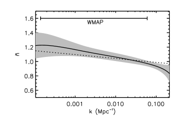
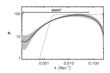
with $k_{0}=0.002$Mpc^-1 for cases A and B. Case A is shown figures (1) and (2), where the former used the WMAP likelihood approximation, and the latter used the ideal likelihood calculation for $\ell\leq 100$ ignoring noise and coupling due to sky cut. Figure (3) shows the one-sigma running (case B). In all the figures, the dashed line denotes the fiducial PPS, and the solid line the mean reconstructed spectrum. Our method successfully recovers the PPS over the WMAP-sensitive scales, and detects a noticeable deviation from $\tilde{n}=1$. The comparison of the two case A reconstructions, figures (1) and (2), shows that the likelihood approximation does not significantly affect the reconstructed spectrum. The bend at low $k$ in figure (3) is due to the prior requiring $\mathcal{P}(k)$ to be greater than ten at the knots. Clearly $\mathcal{P}(k)$ must be positive, but occasionally the interpolating spline between the knots goes negative, and we must discard such steps in the Markov chain. Choosing a lower prior of ten for the knot values helps keep the interpolating spline from going negative. The “sharp cutoff” PPS reconstruction, shown in figure (4), hits a non-negative prior on the PPS knot values more strongly, since splines with steep slopes are more likely to go negative. It resembles a running of the spectral index, showing how our method tends to “smooth out” sharp features.

Figure 1: The spectral index $\tilde{n}(k)$ of the reconstructed PPS from the mock data with a running of $\alpha_{s}=-0.047$ and the best-fit values for the WMAP running spectral index model for the rest of the cosmological parameters. The reconstruction used a smoothing spline with five knots equally spaced in $\ln k$ and no roughness penalty, and the likelihood approximation used by the WMAP team. The dark line denotes the mean, the shaded region denotes one standard deviation, and the dashed line denotes the fiducial PPS.

Figure 2: The spectral index $\tilde{n}(k)$ of the reconstructed PPS from the mock data with a running of $\alpha_{s}=-0.047$ and the best-fit values for the WMAP running spectral index model for the rest of the cosmological parameters. The reconstruction used a smoothing spline with five knots equally spaced in $\ln k$ and no roughness penalty, and an exact likelihood calculation for $\ell=2-100$. The dark line denotes the mean, the shaded region denotes one standard deviation, and the dashed line denotes the fiducial PPS.

Figure 3: The spectral index $\tilde{n}(k)$ of the reconstructed PPS from mock data with a running of $\alpha_{s}=-0.087$ and the best-fit values for the WMAP running spectral index model for the rest of the cosmological parameters. The reconstruction used a smoothing spline with five knots equally spaced in $\ln k$ and no roughness penalty. The dark line denotes the mean, the shaded region denotes one standard deviation, and the dashed line denotes the fiducial PPS. The bend at low $k$ is due to the spectrum hitting the prior.

Figure 4: The reconstructed $\mathcal{P}(k)$ from mock data with a cutoff at $k=0.002$ the best-fit values for the WMAP flat PPS model for the rest of the cosmological parameters. The reconstruction used a smoothing spline with five knots equally spaced in $\ln k$ and no roughness penalty. The dark line denotes the mean, the shaded region denotes one standard deviation, and the dashed line denotes the fiducial PPS.

V PPS Reconstruction Results

We next apply the smoothing spline reconstruction to the combination of the first-year WMAP TT and TE power spectra Kogut et al. (2003); Hinshaw et al. (2003). Our aim here is to test the statistical significance of possible smooth deviations from scale invariance; our “null hypothesis” is a scale-invariant ($n=1$) PPS. Thus, as a benchmark, we run a Markov chain to find the best-fit parameters for such a model. Since the volume of parameter space for wiggly power spectra is far greater than the volume for flat spectra, the Markov chain tends towards more curvy (higher $F$) spectra than flat ones, due to entropy. One may compensate for this effect by increasing $\lambda$, but it is still very unlikely for a Markov chain started from a curved PPS to line up the spline’s knots to retrieve a totally flat $n=1$ spectrum. To minimize burn-in and to make sure our chains include the null hypothesis case, we start the smoothing spline Markov chains from a scale-invariant PPS with cosmological parameters set to the $n=1$ model’s best-fit parameters.

After running several preliminary chains with different numbers of knots and different smoothing parameters, we settled with three well-mixed, converged Markov chains with smoothing splines, one with five knots and roughness penalty $\lambda=0.1$, one with five knots and $\lambda=0$,and one with seventeen knots and roughness penalty $\lambda=2\times 10^{-5}$. We use the roughness parameter of $2\times 10^{-5}$ for the 17-knot spline because it is very tiny constraint on the flexibility of the PPS, but sufficient to allow the Markov chain to converge in a reasonable amount of time.

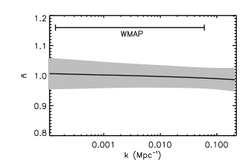
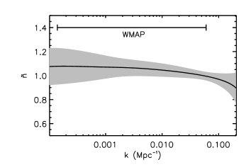
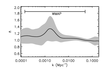
Figure (5) shows the mean spectral index (Eq.(6)) and one-sigma confidence interval for the WMAP data for a smoothing spline with five knots and a smoothing parameter of 0.1. The resulting PPS is indistinguishable from flat. Removing the roughness penalty yields the recovered PPS shown in figure (6), which has a $\Delta\chi^{2}$ of only 1.79 away from flat. Giving the PPS spline a lot more freedom, seventeen knots and a smoothing parameter of only $2\times 10^{-5}$, one recovers the function in figure (7). Although this spline was given much more parameter space and a much lower $\lambda$ than preferred by the data, the one-sigma confidence interval is still consistent with a flat $n=1$ spectrum.

In all these cases, the posterior probability density created by the Markov chains concentrates in regions of low roughness penalty. This implies that the data do not require the additional flexibility of the smoothing spline reconstruction. For all the steps in all our runs with finite $\lambda$, $\lambda F$ remains on the order of 0.1% to 1% of $\ln\mathcal{L}$. This means that moving far away from a flat power spectrum cannot improve the likelihood sufficiently to overcome the roughness penalty.

CV confirms this qualitative interpretation. We ran our $\frac{N}{2}$-fold CV for two different sets of fixed cosmological parameters, the best-fit flat and the five-knot no-lambda best fit, and find an optimum $\lambda\gtrsim 0.1$ for a five-knot spline. Therefore, the PPS should be closer to scale invariant than the five-knot spline with $\lambda=0$ results (figure 6) and at least as close to scale invariant as the five-knot spline with $\lambda=0.1$ (figure 5). Since increasing the number of knots or decreasing $\lambda$ both increase the effective degrees of freedom, we can also conclude that the PPS should be much closer to scale invariant than the 17-knot spline with $\lambda=2\times 10^{-5}$ result (figure 7).

Figure (6) shows a flatter PPS than (1), with the same number of knots and same smoothing parameter ($\lambda=0$). Thus, we conclude that if the PPS had a running of $|\alpha_{s}|\gtrsim 0.05$ the smoothing spline technique applied to WMAP data would have recovered it. The smoothing spline finds no evidence for deviations from a scale invariant power spectrum from WMAP first-year data.

Figure 5: The spectral index $\tilde{n}(k)$ of the PPS reconstructed using a smoothing spline with five knots equally spaced in $\ln k$ and a smoothing parameter of 0.1. The dark line denotes the mean and the shaded region denotes one standard deviation.

Figure 6: The spectral index $\tilde{n}(k)$ of the PPS reconstructed using a smoothing spline with five knots equally spaced in $\ln k$ and no smoothing penalty. The dark line denotes the mean and the shaded region denotes one standard deviation.

Figure 7: The spectral index $\tilde{n}(k)$ of the PPS reconstructed using a smoothing spline with 17 knots equally spaced in $\ln k$ and a smoothing parameter of $2\times 10^{-5}$. The dark line denotes the mean and the shaded region denotes one standard deviation.

V.1 Comparing CV with other criteria

The preference for a very flat PPS, indicated by the spline reconstruction and its CV, can be cross-checked with alternative model-testing techniques, such as Bayesian evidence.

We apply the Akaike information criterion (AIC) and Bayesian information criterion (BIC) to compare the five-knot, $\lambda=0$ spline with the scale invariant model. These methods are improvements on the standard likelihood ratio test Kendall and Stuart (1969) in that they rely on fewer assumptions Liddle (2004). Both criteria add a penalty for additional degrees of freedom to the negative log likelihood, so that a lower value for this sum indicates the preferred model. The AIC Akaike (1974) comes from an approximation to the Kullback-Leiber information entropy, used to measure the difference in goodness of fit between two models. The BIC Schwarz (1978) approximates the Bayes factor, or the ratio of the likelihood of two models with a flat initial prior. The BIC has a more stringent requirement to accept extra parameters than the AIC Liddle (2004). Here we find that both criteria prefer the simpler, scale-invariant model; see table (1). A difference in BIC of ten or more is considered very strong evidence for the preferred model, and here we have a difference of twenty-six favoring the flat spectrum over the five-knot spline. Even the weaker AIC prefers the simpler model by a difference of six.

Our results are consistent with previous work applying Bayesian evidence to determine the significance of the spectral index $n$ in the cosmological parameter set (versus setting $n=1$). Liddle Liddle (2004) applies the AIC and BIC and finds that the data favor the simpler scale-invariant model. Trotta Trotta (2005) uses the Laplace and Savage-Dickey approximations to the Bayes factor, and finds 2:1 odds in favor of the Harrison-Zeldovich spectrum using CMB data. Our tests extend these results and compare the Harrison-Zeldovich model to shapes with more flexibility than the one free parameter $n$.

	5-knot spline	minimal ($n$=1)
AIC	1448	1442
BIC	1494	1468

Table 1: The Akaike information criterion and Bayesian information criterion applied to the five-knot smoothing spline PPS with zero lambda and the minimal cosmological model. Since preferred models have lower AIC and BIC, both criteria prefer the minimal model.

VI Sensitivity of Cosmological Parameters on the PPS

	5-knot spline	17-knot spline	power law	running	minimal ($n$=1)
$\Omega_{b}h^{2}$	0.021$\pm$0.002	0.022$\pm$0.004	0.024$\pm$0.001	0.023$\pm$0.002	0.0240$\pm$0.0004
$\Omega_{m}h^{2}$	0.14$\pm$0.02	0.14$\pm$0.03	0.14$\pm$0.02	0.14$\pm$0.02	0.15$\pm$0.02
$h$	0.67$\pm$0.06	0.63${}^{+0.18}_{-0.10}$	0.72$\pm$0.05	0.70$\pm$0.05	0.70$\pm$0.05
$\tau$	0.21${}^{+0.08}_{-0.10}$	0.26${}^{*}_{-0.08}$	0.166${}^{+0.076}_{-0.071}$	0.20$\pm$0.07	0.18$\pm$0.05

Table 2: Cosmological parameters and errors recovered by smoothing spline PPS’s versus the WMAP results Spergel et al. (2003) for a power law and running spectral index PPS and an $n$=1 PPS. The values and errors for $\Omega_{m}$ remain quite independent of PPS flexibility. Allowing smooth features in the PPS loosens the constraints on $\Omega_{b}$, $h$, and $\tau$. * denotes hitting the prior.

Because the measured CMB power spectrum depends nonlinearly on both the PPS and the cosmological parameters, there are degeneracies between the PPS shape and the cosmological parameters. We now investigate how the increased freedom in the PPS allowed by the spline technique affects the recovered values of the cosmological parameters. Similar analyses yielding qualitatively similar results using multiple CMB data sets, large-scale structure, and piecewise and band-power PPS reconstructions, can be found in Bridle et al. (2003); Mukherjee and Wang (2003a).

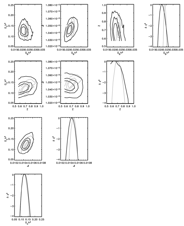
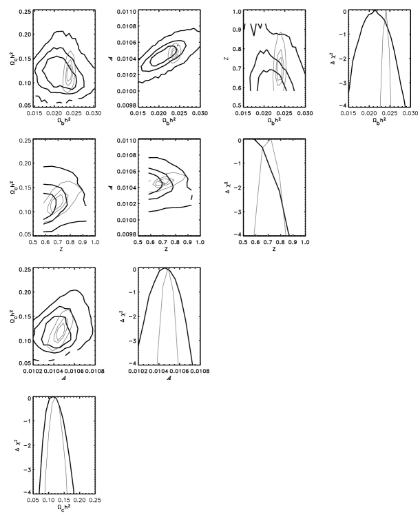
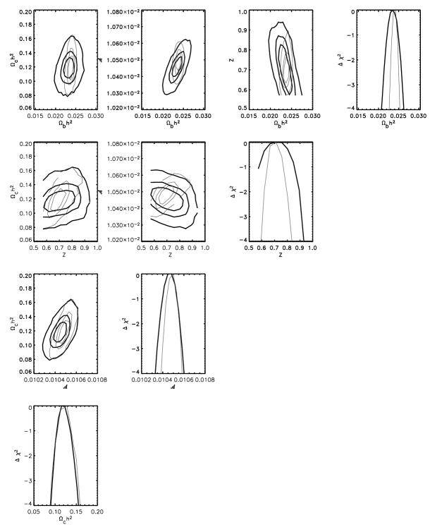
Figure (8) (dark lines) shows the cosmological parameter likelihood contours for the one sigma marginalized, one sigma joint, and two sigma joint confidence intervals for the five-knot spline with no lambda, figure (9) shows the same for the seventeen-knot spline with $\lambda=2\times 10^{-5}$, and figure (10) shows the same for the five-knot spline with $\lambda=0.1$ . For comparison, the thin gray lines in each figure show the likelihood contours when the PPS is forced to be Harrison-Zeldovich.

We find that the best-fit values for all parameters except $Z$ do not significantly change as the PPS is allowed more freedom compared to the scale-invariant case. The error bars increase, however, especially in the 17-knots case.

Table (2) shows the values and errors for the cosmological parameters for our two smoothing spline reconstructions compared to the WMAP errors Spergel et al. (2003) and the minimal model ($n=1$) errors. The parameter that shows least sensitivity to the increased flexibility in the PPS is $\Omega_{m}h^{2}$, followed by ${\cal A}$. These parameters are the least degenerate with smooth features in the PPS. The increased freedom in the PPS increases the errors significantly (by a factor $\sim 5$ for the five-knot case compared to the Harrison-Zeldovich case) for $\Omega_{b}h^{2}$. Drastic changes are also observed in the likelihood contours for $Z$. Following the WMAP team Spergel et al. (2003), we have imposed a hard prior on $\tau$ of $\tau<0.3$. While the effect of this prior is not very important for the scale-invariant case, it sharply cuts the likelihood contours in the spline cases. As additional freedom in the PPS is allowed, the recovered best-fit value for $\tau$ is pushed towards the limit imposed by the prior. With only the TT and TE power spectra, the optical depth is significantly degenerate with the PPS shape. We expect the addition of EE polarization power spectrum will break this degeneracy.

Figure 8: Errors on cosmological parameters from a Markov chain run for a smoothing spline $\mathcal{P}$ with five knots and no roughness penalty. Dark contours denote one sigma marginalized, one sigma joint, and two sigma joint. Over-plotted with thin, gray contours are the errors for a $n=1$ flat PPS for comparison. $\Omega_{b}$ is the baryon fraction, $\Omega_{c}$ is the cold dark matter density, ${\cal A}$ is the present angular size of the sound horizon at the last scattering surface, and $Z=e^{-2\tau}$ where $\tau$ is the optical depth.

Figure 9: Errors on cosmological parameters from a Markov chain run for a smoothing spline $\mathcal{P}$ with 17 knots and and a smoothing parameter of 2x$10^{-5}$. Dark contours denote one sigma marginalized, one sigma joint, and two sigma joint. Over-plotted with thin, gray contours are the errors for a $n=1$ flat PPS for comparison. $\Omega_{b}$ is the baryon fraction, $\Omega_{c}$ is the cold dark matter density, ${\cal A}$ is the present angular size of the sound horizon at the last scattering surface, and $Z=e^{-2\tau}$ where $\tau$ is the optical depth.

Figure 10: Errors on cosmological parameters from a Markov chain run for a smoothing spline $\mathcal{P}$ with 5 knots and and a smoothing parameter of 0.1. Dark contours denote one sigma marginalized, one sigma joint, and two sigma joint. Over-plotted with thin, gray contours are the errors for a $n=1$ flat PPS for comparison. $\Omega_{b}$ is the baryon fraction, $\Omega_{c}$ is the cold dark matter density, ${\cal A}$ is the present angular size of the sound horizon at the last scattering surface, and $Z=e^{-2\tau}$ where $\tau$ is the optical depth.

VII Conclusions

Cosmological data now offer the ability to go beyond finding preferred parameters under a given model, and to compare the success and statistical preference for different models. Here we have used a nonparametric (or minimally parametric) method to test a subset of smooth PPS models. We have presented smoothing spline reconstructions of the PPS using CMB data, complementary to other nonparametric reconstructions presented in the literature. We applied this technique to WMAP first-year data.

The smoothing spline reconstruction gives the PPS significantly more freedom than a power-law or a running spectral index model, and is poised to recover smooth features in the PPS. We find that the spline is not sensitive to small, sharp features in the PPS, but if a feature such as a running of the spectral index $\alpha_{s}\gtrsim-0.05$ is present in WMAP first-year data, the technique can recover it.

We first reconstructed the PPS without any roughness penalty with a five-knot spline, thus leaving the PPS four extra degrees of freedom compared to a scale-invariant $n=1$ model. Then, to quantitatively assess if the data require extra effective degrees of freedom in the PPS, we used three different statistical tests. We first applied cross validation, the standard statistical method for choosing a smoothing spline’s smoothing parameter. We found that CV prefers a high smoothing parameter, indicating a preference for a flat (scale-invariant) PPS. We then compared this result with the AIC and BIC, information criteria for measuring the statistical significance of additional parameters in a model. Both the AIC and BIC strongly indicate no preference for the extra freedom of the smoothing spline.

Thus, we found no statistically significant indications for any deviations from a scale invariant ($n=1$) PPS. We find that most cosmological parameters, especially the matter density $\Omega_{m}$, remain fairly robust to flexibility in the PPS. However, the constraints on $\Omega_{b}h^{2}$ and to a greater extent on the optical depth $\tau$ are significantly weakened. We expect that the addition of EE-polarization data will break the degeneracy between optical depth and the PPS shape. Large-scale structure data, which now overlaps the scales of the CMB data, could help even more in constraining the cosmological parameters when the PPS is flexible. Here we have shown that even using CMB data alone, the cosmological parameters are quite robust. Our results are consistent with Mukherjee and Wang (2003a) and Bridle et al. (2003). In particular, we find roughly the same increases in errors and changes in the values of the cosmological parameters as Mukherjee and Wang’s Mukherjee and Wang (2003a) PPS reconstructions using 11 wavelet band-powers and top-hat bins and CMB data only. The addition of large-scale structure data naturally shrinks the errors slightly.

The smoothing spline is a statistically rigorous tool, and has a solid Bayesian justification when applied to direct measurements of the sought-after function Wahba (1990); Green and Silverman (1994). We had to modify the smoothing spline method due to the complicated transfer function between the CMB data and the PPS. With more computing power or faster methods to compute the theory $C_{\ell}$ (such as CMBwarp Jimenez et al. (2004)), we could, in theory, include as many knots as data points, and perform one-fold CV to choose the optimum smoothing parameter. Such a reconstruction would be able to soundly detect features as fine as the data could possibly distinguish.