Which physical parameters can be inferred
from the emission variability of relativistic jets?

We present results of a detailed numerical study and theoretical analysis of the dynamics of internal shocks in relativistic jets and the non-thermal flares associated with these shocks. In our model internal shocks result from collisions of density inhomogeneities (shells) in relativistic jet flows. We find that the merged shell resulting from the inelastic collision of shells has a complicated internal structure due to the non-linear dynamics of the interaction. Furthermore, the instantaneous efficiency for converting kinetic energy into thermal energy is found to be almost twice as high as theoretically expected during the period of significant emission. The Lorentz factors of the internal shocks are correlated with the initial inertial masses of the shells.

Because of the complexity of the non-linear evolution the merged shell becomes very inhomogeneous and simple one-zone models are inadequate to extract physical parameters of the emitting region from the resulting light curves. In order to improve on these one-zone approximations, we propose a novel way of analyzing the space-time properties of the emission. Based on these properties we construct an analytic model of non-thermal flares which can be used to constrain some (unobservable) physical parameters of the internal shocks. These are the ratio of the Lorentz factors between the forward and the reverse shock (caused by the shell collision), and the shell crossing times of these shocks. The analytic model is validated by applying it to the synthetic light curves computed from our models. It can equally well be applied to observations.

1 Introduction

BL Lac objects are a class of active galactic nuclei (AGN) which show the most rapid variability of all AGNs. In the X-ray frequency range they display flares whose duration in the observer frame is usually of the order of one day (Maraschi et al. 1999, Takahashi et al. 2000, Kataoka et al. 2001), as further confirmed by the longterm observation of Mrk 501, PKS 2155-304, and Mrk 421 (Tanihata et al. 2001, Tanihata 2001). With the highly improved sensitivity of $XMM-Newton$, variability on time scales down to a few kiloseconds could be studied in Mrk 421 (Brinkmann et al. 2001, 2003) and only recently, from an $XMM-Newton$observation of Mrk 421 in a very high state, the spectral evolution of the object down to time scales of $\geq$ 100 sec could be followed (Brinkmann et al. 2005).

The internal shock scenario (Rees & Mészáros 1994) is usually invoked in order to explain the variability of blazars (Spada et al. 2001, Bicknell & Wagner 2002). These shocks are typically assumed to arise due to the collisions of density inhomogeneities within the relativistic blazar jets. Recently, one–dimensional (Kino et al. 2004) and two–dimensional (Mimica et al. 2004; thereafter MAMB04) simulations of such internal shocks have been performed both showing that the evolution of internal shocks is considerably more complicated than what has been concluded from approximate analytic considerations. As a result of the complexity of the non-linear evolution arising after a two-shell interaction, the merged structure becomes very inhomogeneous and simple one-zone models are inadequate to extract physical parameters of the emitting region from the resulting light curves. In particular, we will show that the rest-mass density of the emitting shell can hardly be inferred from fits to the synthetic light curves. Assuming an approximately uniform proportionality between the rest-mass energy and the magnetic field energy the magnetic field strength might hardly be inferred from a flare light curve, too. Should the evolution of real shell interactions be as complex, the parameters obtained from one-zone model fits to the spectra will be equally inaccurate as those obtained from one-zone model fits of the light curves.

In this paper we both extend our simulations of internal shocks and perform a systematic study of the influence of the fluid properties on the formation of flares, on their duration and temporal profiles, and develop an analytic model linking the fluid properties to the observed flare properties. One of the advantages of our analytic model is that it can be validated by comparing its predictions to the actual physical conditions obtained from our relativistic hydrodynamic simulations. This validation will probe to be very important considering the disparity of physical values predicted by other analytic models for single flares in certain blazars (see § 7).

In section § 2 we discuss the internal shock scenario as a model which explains the flare emission and we summarize our previous findings (MAMB04) regarding the hydrodynamic evolution of internal shocks. The numerical simulations are described in Section § 3. Finally, in § 4 we present an analytic model which can be used to infer physical parameters of the fluid flow from either synthetic or observed flare light curves (§ 5 and 6).

2 Internal shock scenario

The internal shock scenario assumes the existence of blobs of matter moving with different velocities along the jet, presumably emitted by the intermittently working central engine. Two blobs will interact after a certain time depending on their initial relative velocity. Once the interaction of the shells starts two internal shocks form, one propagating into the slower shell (forward shock) and another one into the faster shell (reverse shock). The interaction of the blobs is modeled as a collision of two homogeneous shells (Spada et al. 2001, Tanihata et al. 2003), and also directly simulated (MAMB04). These models shells are assumed to have sharp edges (density discontinuities) separating them from the background fluid.

The present work relies on the physical model developed by MAMB04. In that model the comoving magnetic field in the region behind the shocks is assumed to be randomly oriented in space. Its energy density is proportional to the internal energy density of the shocked fluid. The non-thermal particles simulated within the model are accelerated at the shock front to very high Lorentz factors whereby they radiate synchrotron radiation.

The observed light curve from a two-shell collision depends on the position along the jet at which the interaction occurs as well as on the details of the evolution. As we discussed in MAMB04, the hydrodynamic evolution of the shells begins already before the collision time predicted by the analytic models (e.g. Spada et al. 2001) and its most important features are (MAMB04):

• The front (with respect to the direction of motion) discontinuity of each shell decays into a bow shock, a contact discontinuity and a reverse shock.

• The back discontinuity of each shell develops into two rarefactions. The first one connects the still unperturbed material inside the shell with a contact discontinuity separating shell matter and external medium. The second rarefaction connects the contact discontinuity with the external medium.

The pre–collision evolution is quantitatively similar independent of whether the edges of the colliding shells are modeled as sharp discontinuities or by a smooth transition layer. The pre-collision evolution of the shells is important as the internal energy of the front part of the shells rises due to the supersonic propagation of the shells. Hence, when they actually start colliding the conditions inside the shells are different from those at ejection from the central engine, i.e., the conditions at the contact surfaces of the two shells are different from those of the initial shells. Once the shells start to collide the evolution consists of three basic stages:

• The pressure in the region between the two shells rises rapidly (compared to the light crossing time of the shell). The front and the reverse shock propagate into the slower and faster shell, respectively.

• The shocks heat up the cold shell material. While the heated region expands the pressure decreases slightly.

• The front shock breaks out of the slower shell, enters the less dense external medium, and thus accelerates. The pressure decreases more rapidly during this stage because of the faster expansion.

3 Numerical simulations

In our previous paper we simulated shell collisions in two spatial dimensions. The results showed that the lateral expansion is negligible during the collision of aligned shells (MAMB04, Fig. 4). Thus, all essential features of aligned shell interactions can be captured using 1D simulations. This allowed us to compute seven high-resolution 1D models all having the same initial shell velocities and the same shell geometries. The models include one where the rest mass densities of both shells are identical (S10-F10), two where both shells have approximately the same conserved mass (S10-F07, S14-F10), and one where both shells possess the same kinetic energy (S10-F05). The latter three models were also simulated by exchanging the initial rest mass density of the colliding shells (Tab. 1).

sim.	$\displaystyle{\frac{\rho_{1}}{10^{3}\rho_{\rm ext}}}$	$\Gamma_{1}$	$\displaystyle{\frac{{\cal M}_{1}}{10^{3}\rho_{\rm ext}V}}$	$\displaystyle{\frac{\rho_{2}}{10^{3}\rho_{\rm ext}}}$	$\Gamma_{2}$	$\displaystyle{\frac{{\cal M}_{2}}{10^{3}\rho_{\rm ext}V}}$	$\Gamma_{\rm b}^{\rm sim}$	$\Gamma_{\rm f}^{\rm sim}$
S10-F10	$1$	$5$	$5$	$1$	$7$	$7$	$5.70$	$6.04$
S10-F07	$1$	$5$	$5$	$0.7$	$7$	$4.9$	$5.61$	$5.97$
S10-F05	$1$	$5$	$5$	$0.5$	$7$	$3.5$	$5.52$	$5.89$
S10-F14	$1$	$5$	$5$	$1.4$	$7$	$9.8$	$5.78$	$6.12$
S07-F10	$0.7$	$5$	$3.5$	$1$	$7$	$7$	$5.79$	$6.12$
S05-F10	$0.5$	$5$	$2.5$	$1$	$7$	$7$	$5.88$	$6.20$
S14-F10	$1.4$	$5$	$7$	$1$	$7$	$7$	$5.61$	$5.96$

Table 1: Overview of the shell properties (densities $\rho_{1}$ and $\rho_{2}$, Lorentz factors $\Gamma_{1}$ and $\Gamma_{2}$, and inertial masses ${\cal{M}}_{1}$ and ${\cal M}_{2}$) of the seven 1D models. The initial thickness of the shells is $10^{14}$ cm, their volume is $V$, and their initial separation is $D_{0}=10^{14}$ cm. The density of the external medium $\rho_{\rm ext}=10^{-23}$ g cm^-3, and its Lorentz factor $\Gamma_{\rm ext}=2.9$. Initially $p/\rho c^{2}=10^{-4}$ everywhere. The parameters of the type–E shock acceleration model (see MAMB04 for details) are: $\alpha_{\rm e}=10^{-2}$, $\gamma_{\rm min}=30$, $\eta=7\,10^{3}$. The last two columns give the Lorentz factor of the reverse ($\Gamma_{\rm b}^{\rm sim}$) and forward ($\Gamma_{\rm f}^{\rm sim}$) shocks, computed from the hydrodynamic simulations.

The numerical grid consists of $10^{4}$ zones covering a physical domain with a length of $5\,10^{15}$ cm. A re-mapping technique (see MAMB04 for details) was applied in order to be able to follow the evolution of the two shells initially separated by $10^{14}$ cm up to distances of $10^{17}$ cm from the AGN engine. The re-mapping technique allowed us to resolve spatial scales from $5\,10^{11}$ cm to $10^{17}$ cm.

The energy distribution of the non–thermal electrons is covered by 64 energy bins, and the number of frequencies at which we compute the synchrotron radiation is $25$, logarithmically spanning the frequency range from $10^{16}$ to $10^{19}$ Hz. We use the type-E shock acceleration model of MAMB04.

The integration of the conservation laws of relativistic hydrodynamics and the computation of the synchrotron radiation are performed using RGENESIS, which is an extension of the code GENESIS (Aloy et al. 1999). The handling of the non–thermal particles within RGENESIS is described in detail in MAMB04.

3.1 Hydrodynamic evolution

The main properties of the hydrodynamic evolution of our models are summarized in Figs. 1 and 2 showing the initial models (top row), the formation of the internal shocks (middle row), and the final state (bottom row).

Figure 1: Hydrodynamic evolution of the shell collision for models S10-F10, S10-F14, S10-F07, and S10-F05. The solid lines give the rest mass density in units of $\rho_{\rm ext}$. The dashed lines show the Lorentz factor of the fluid which is moving to the right. The origin of the z-axis corresponds to a distance of 0 cm (top row), $2.65\,10^{16}$ cm (middle row), and $6.61\,10^{16}$ cm (bottom row), respectively. Times given in the leftmost panels of each row are measured in the laboratory frame.

Figure 2: Same as Fig. 1, but for models S14-F10, S07-F10 and S05-F10. Model S10-F10 is shown once again here to allow for an easier comparison.

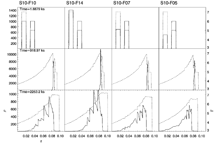
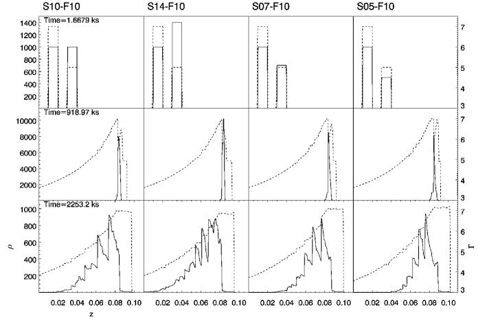
The evolution depends on the density of the shells in the following way: the higher the density of the faster shell, the higher is the resulting density peak (middle rows of Figs. 1 and 2), and the larger are the density variations within the merged shell (bottom rows in Figs. 1 and 2). The shock Lorentz factors, as computed from the simulations ($\Gamma_{\rm b}^{\rm sim}$, $\Gamma_{\rm f}^{\rm sim}$), increase with the rest mass density of the faster shell.

Kino et al. (2004) obtain a multi–peaked final density distribution, which they attribute to the rarefaction waves forming when the internal shocks cross the edges of the shells. In our models the rarefaction waves cause the Lorentz factor to decrease towards the rear part of the merged shell (bottom rows in Figs. 1 and 2). However, the direct comparison with Kino et al.  (2004) is difficult, as their results are computed in the comoving frame of the contact discontinuity between the two shells, whereas our results are shown in the laboratory frame attached to the central engine. Despite of this difficulty, there is a robust result common to every simulation modeling two-shell interactions, namely the formation of a very inhomogeneous merged structure as a result of the non-linear evolution of the system. This heterogeneity flaws simple one-zone models assuming homogeneous conditions in the emitting regions.

3.2 Energy conversion efficiency

Assuming an inelastic collision of two shells, the following conversion efficiency $\epsilon$ of bulk kinetic energy into internal energy can be derived from the conservation of energy and momentum (Kobayashi et al.  1997; Daigne & Mochkovitch  1998):

$$\epsilon=1-\displaystyle{\frac{({\cal M}_{1}+{\cal M}_{2})\Gamma_{m}}{{\cal M}_{1}\Gamma_{1}+{\cal M}_{2}\Gamma_{2}}}\,,$$ (1)

where ${\cal M}_{i}=\rho_{i}\Gamma_{i}V$ is the total inertial mass of the shell $i$ ($i=1,2$), and where the Lorentz factor of the merged shell is given by

$$\Gamma_{m}=\sqrt{\Gamma_{1}\Gamma_{2}\displaystyle{\frac{{\cal M}_{1}\Gamma_{1}+{\cal M}_{2}\Gamma_{2}}{{\cal M}_{1}\Gamma_{2}+{\cal M}_{2}\Gamma_{1}}}}\,.$$ (2)

The (time independent) efficiency given in Eq. (1) corresponds to a situation where two incompressible shells collide inelastically and instantaneously. However, as we are modeling the shells as compressible fluids, we have to consider the temporal evolution of the energy conversion efficiency, and hence use the following generalized definition

$$\epsilon(T)\equiv 1-\displaystyle{\frac{\int\Gamma^{2}(T,z)\rho(T,z){\rm d}z}{\int\Gamma^{2}(0,z)\rho(0,z){\rm d}z}}\,,$$ (3)

where $\rho(T,z)$ and $\Gamma(T,z)$ are the rest mass density and the Lorentz factor of the fluid at a time $T$ at position $z$, respectively. We point out that the instantaneous values of $\epsilon(T)$ do not necessarily coincide with those given by Eq. (1), because during the hydrodynamic evolution the fluid suffers multiple compressions and expansions changing the ratio of internal energy and kinetic energy (which is assumed to be constant in the simple model).

Figure 3: Temporal evolution of the conversion efficiency defined by Eq. (3) for all models. $T$ is the time measured in the source frame.

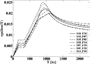
Fig. 3 shows the temporal evolution of conversion efficiency $\epsilon(T)$ for all of our simulated models. Initially, the efficiency rises until about $150$ ks, and then remains nearly constant until $350$ ks. The analysis of the hydrodynamic evolution shows that this is due to the fact that the faster shell is heated due to its interaction with the medium ahead of it. However, at $150$ ks the shell encounters a rarefaction created by the slower shell reducing the amount of heating. At $330$ ks the internal shocks form and the efficiency starts rising again until it reaches a maximum at about $1000$ ks. The subsequent decrease of the efficiency is caused by the expansion of the fluid as the shocks break out of and rarefactions form within the merged shell. The efficiency is generally the higher the smaller is the rest-mass density of the faster shell (Tab. 2). We note that the final values approach the efficiency predicted by the conservation laws (Eq. (1)).

sim.	$\epsilon_{\rm max}$	$\epsilon_{\rm fin}$	$\epsilon_{\rm pred}$
S10-F10	$0.0220$	$0.0133$	$0.0136$
S10-F07	$0.0241$	$0.0137$	$0.0140$
S10-F05	$0.0250$	$0.0138$	$0.0135$
S10-F14	$0.0198$	$0.0123$	$0.0125$
S07-F10	$0.0210$	$0.0142$	$0.0125$
S05-F10	$0.0200$	$0.0149$	$0.0109$
S14-F10	$0.0225$	$0.0121$	$0.0140$

Table 2: Maximum conversion efficiency $\epsilon_{\rm max}$, final conversion efficiency $\epsilon_{\rm fin}$, and theoretically predicted conversion efficiency $\epsilon_{\rm pred}$ (see Eq. (1)) for the seven simulated models.

The time evolution of the conversion efficiency in our models is qualitatively similar to that of Kino et al. (2004). However, due to the fact that these authors computed the evolution in the rest frame of the (relativistically moving) contact discontinuity, a quantitative comparison with our results is presently impossible.

3.3 Synthetic light curves

Figure 4: Soft (upper panel; observed photon energies between $0.1$ and $1$ keV) and hard (lower panel; $2$-$10$ keV) light curves for all of our seven models. A correlation between the total rest-mass of the shells and the peak photon counts is seen.

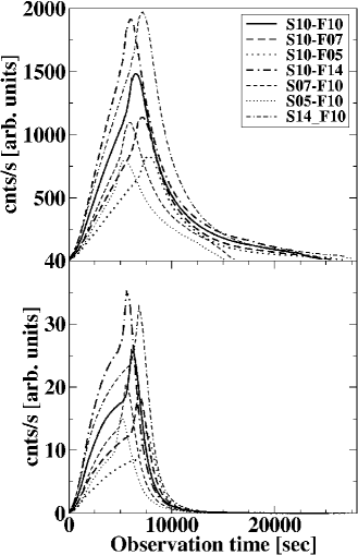
The peak intensity of the light curves in both the soft (Fig. 4; upper panel; $0.1-1$ keV) and the hard energy band (Fig. 4; lower panel; $2-10$ keV) is correlated to the total rest-mass of the shells (see Tab. 1). This correlation is slightly better in the wider hard energy band. We further find that the peak of the flare occurs in the hard energy band several hundreds of seconds before the peak in the soft band.

The shape of the flares is qualitatively similar for all models indicating that the variation of the density ratio between shells mostly tends to change the normalization of the flares. Furthermore, the large variations of the density (Figs. 1 and 2 bottom rows) and of the specific internal energy are not correspondingly do not change the shape of the light curves which are rather smooth. This implies that from the shape of the flare alone, it is very hard to infer any information about the rest–mass density or the specific internal energy of the emitting regions. This restriction should be taken into account by any analytic model aiming to infer physical parameters from light curves.

3.4 Sensitivity to the initial conditions

The light curves generated from our models are rather insensitive to both the choice of density and pressure of the external medium provided they are sufficiently small to be inertially negligible. If the density of the underlying medium is comparable to that of the shells the evolution will be quantitatively different (but qualitatively, the same Riemann structure will develop from every edge of every shell). We have limited the Lorentz factor of the external medium to be smaller than that of the slowest shell. Its value changes only the depth of the rarefaction trailing both shells (the smaller the velocity of the jet, the smaller the pressure and the density reached behind every shell). However, this will not change the light curves of our models as from rarefactions there is no emission (because only shocked regions emit in our model). The complementary situation, i.e., one or both shells being slower than the jet, we have not considered. This situation will correspond to a couple of shells being slower than the underlying, light jet. In such a case, the Riemann structure will be qualitatively different. The rear edges of the shells will be heated because of the development of shocks while the pull of the external medium will create rarefactions from the forward edges of every shell. Nevertheless, this interesting situation falls beyond the scope of the current work and will be considered elsewhere. We point out that it is reasonable to expect a low–density external medium, since the shells will clean up the medium through which they propagate (note that the state left behind every shell is less dense than that set up initially). This rarefication process of the external medium is a robust feature associated with the shell motion (see MAMB04).

4 Analytic modeling of flares

In this section we discuss some analytic approaches to the modeling of flares resulting from internal shocks, and most importantly which physical parameters can be obtained by analyzing the shape and duration of flares. We begin with general considerations of the observations of distant unresolved sources, and then provide an analytic model particularly suited to study the flares resulting from collisions of shells in a relativistic jet.

4.1 Computation of the radiation observed by a distant observer

As the simplest case, we assume that we have a source of radiation moving along the line–of–sight (LOS) towards a distant observer. We introduce two inertial frames: the source frame and the observer frame. The source frame is attached to the central energy source. In this frame the physics of the source is best described because time and space are independent coordinates. In the source frame, we denote the position along the LOS by $z$, and the time by $T$. The observer frame is located at a distance $z=z_{\rm obs}$ along the LOS. Except for a cosmological redshift factor, this frame is equivalent to one attached to the Earth. In this frame we have chosen two different coordinate systems, the $(z_{\rm obs},t_{\rm obs})$–system and the $(x,y)$–system. The second coordinate system is best suited for describing the structure of the observations in space time because the coordinates associated with this frame mix the spatial ($z$) and temporal ($T$) coordinates of the source frame in the following way:

$$x=\displaystyle{\frac{cT-z}{\sqrt{2}}}\,,$$ (4)

$$y=\displaystyle{\frac{cT+z}{\sqrt{2}}}\,,$$ (5)

where $c$ is the speed of light.

A process which takes place at time $T$ and position $z$ in the source frame is observed in the observer frame at a time

$$t_{\rm obs}=T+\displaystyle{\frac{z_{\rm obs}-z}{c}}=\displaystyle{\frac{\sqrt{2}x}{c}}+\displaystyle{\frac{z_{\rm obs}}{c}}\,,$$ (6)

i.e., all points with the same $x$ coordinate will be observed simultaneously. Hence, the total radiation observed by a distant observer at time $t$ is equal to the integral over $y$ of the emitted radiation of all points in the source frame which have the same $x=(ct-z_{\rm obs})/\sqrt{2}$ coordinate in the observer frame ($xy$–coordinate system), i.e.,

$$I(t)=\int{\rm d}y\,j(x,y)\,,$$ (7)

where $I(t)$ is the intensity of the observed radiation at time $t$, and $j(x,y)$ is the emissivity in the observer frame. This emissivity is related to the emissivity at the corresponding time and place in the source frame, i.e., $j(x,y)=j(z(x,y),T(x,y))$.

If a point source is moving with a velocity $\beta c$ then $z(T)=z_{0}+\beta cT$, and its trajectory in $xy$-coordinates will be

$$y(x)=\displaystyle{\frac{1+\beta}{1-\beta}}x+\displaystyle{\frac{\sqrt{2}}{1-\beta}}z_{0}\,.$$ (8)

Hence, an object moving with the speed of light is observed to propagate parallel to the $y$ axis, while an object at rest in the source frame is observed to move parallel to the line $y=x$.

Now we assume that an observer is located at $z_{\rm obs}=0$, and that the emissivity of a point source is a function of the time $T$,

$$j(z,T)=\left\{\begin{array}[]{ll}I_{0}\delta(z-z_{0}-\beta cT)&{\rm if\,}0\leq T\leq T_{\rm end}\\[11.38109pt] 0&{\rm otherwise}\end{array}\right.$$ (9)

where $I_{0}$, $z_{0}$, $\beta$ and $T_{\rm end}$ are the normalization of the emissivity, the initial source position, its velocity in units of the speed of light, and the duration of its emission, respectively. In the observer frame ($xy$-coordinates) the emissivity is then, using (4), (5), and the properties of the $\delta$-function,

$$\begin{array}[]{cc}j(x,y)=&\displaystyle{\frac{I_{0}\sqrt{2}}{1-\beta}}\delta\left[y-\displaystyle{\frac{x(1+\beta)+z_{0}\sqrt{2}}{1-\beta}}\right]\times\\ &S(y;-x,\sqrt{2}cT_{\rm end}-x)\end{array}$$ (10)

where

$$S(x;a,b)=\left\{\begin{array}[]{ll}1&{\rm if\,}a\leq x\leq b\\[11.38109pt] 0&{\rm otherwise}\end{array}\right.\,.$$ (11)

Using now equation (7) we can compute the light curve produced by a single emitting point source observed by a distant observer:

$$I(t)=\displaystyle{\frac{I_{0}\sqrt{2}}{1-\beta}}S\left(\displaystyle{\frac{ct}{\sqrt{2}}};\displaystyle{\frac{-z_{0}}{\sqrt{2}}},\displaystyle{\frac{(1-\beta)cT_{\rm end}-z_{0}}{\sqrt{2}}}\right)\,.$$ (12)

It follows from Eq. (12) that for the observer the duration of the emission is given by

$$t_{\rm total}=(1-\beta)T_{\rm end}\,,$$ (13)

or, in the ultra-relativistic limit by $t_{\rm total}\approx T_{\rm end}/(2\Gamma^{2})$, where $\Gamma=1/\sqrt{1-\beta^{2}}$ is the Lorentz factor of the emitting point source.

This shows that the total time (measured in the source frame) during which the source emits and its Lorentz factor are degenerate for a distant observer, i.e., it is not possible to determine both the Lorentz factor and the source frame time of an emission process from the duration of the observed emission alone. This is a major obstacle for any model which attempts to reconstruct, from an observed flare, the sizes and the velocities of colliding shells which produce that flare. Nevertheless, in the following sections we develop an analytic model which can recover some of the properties of the colliding shells, taking into account this limitation.

4.2 Geometry of the emitting region

Motivated by the results of numerical simulations (MAMB04) the emitting flare can be represented as a horn–shaped region in the observer frame when using the $xy$-coordinates (Fig. 5). The two curves $y_{\rm b}(x)$ and $y_{\rm f}(x)$ delimiting the horn–shaped region correspond to the front and back edges of the merged shell, respectively. They are approximated by second order polynomials passing through the origin (Fig. 5). This leaves two free parameters for each curve, which are determined by requiring that the velocities of the front and back edges be $\beta_{\rm fi}$ and $\beta_{\rm bi}$ at $T=0$, and $\beta_{\rm fe}$ and $\beta_{\rm be}$ at $T=T_{\rm e}$, respectively. $T_{\rm e}$ is the time (measured in the source frame) at which the emissivity from the shell interaction drops below the observable level. By computing the equations of motion (in the observer frame) $z_{\rm f}(T)$ and $z_{\rm b}(T)$ corresponding to $y_{\rm f}(x)$ and $y_{\rm b}(x)$, respectively, one obtains the following equations for the front edge,

$$y_{\rm f}(x)=4\Gamma_{\rm f}^{2}x\left[K_{\rm f}\Gamma_{\rm f}^{2}\displaystyle{\frac{x}{\sqrt{2}T_{\rm e}}}+1-\displaystyle{\frac{1}{4\Gamma_{\rm f}^{2}}}\right]\,,$$ (14)

$$z_{\rm f}(T)=cT\left\{1-\left[\Gamma_{\rm f}^{2}\left(1+\sqrt{1+K_{\rm f}\displaystyle{\frac{T}{T_{\rm e}}}}\right)\right]^{-1}\right\}\,,$$ (15)

and the back edge

$$y_{\rm b}(x)=4\Gamma_{\rm b}^{2}x\left[K_{\rm b}\Gamma_{\rm b}^{2}\displaystyle{\frac{x}{\sqrt{2}T_{\rm e}}}+1-\displaystyle{\frac{1}{4\Gamma_{\rm b}^{2}}}\right]\,,$$ (16)

$$z_{\rm b}(T)=cT\left\{1-\left[\Gamma_{\rm b}^{2}\left(1+\sqrt{1+K_{\rm b}\displaystyle{\frac{T}{T_{\rm e}}}}\right)\right]^{-1}\right\}\,,$$ (17)

where $\Gamma_{\rm f}$, $\Gamma_{\rm b}$, $K_{\rm f}$, and $K_{\rm b}$ are defined as

$$\Gamma_{\rm f}\equiv\left[2\left(1-\beta_{\rm fi}\right)\right]^{-1/2}\,,$$ (18)

$$\Gamma_{\rm b}\equiv\left[2\left(1-\beta_{\rm bi}\right)\right]^{-1/2}\,,$$ (19)

$$K_{\rm f}\equiv\left(\displaystyle{\frac{1-\beta_{\rm fi}}{1-\beta_{\rm fe}}}\right)^{2}-1\,,$$ (20)

$$K_{\rm b}\equiv\left(\displaystyle{\frac{1-\beta_{\rm bi}}{1-\beta_{\rm be}}}\right)^{2}-1\,.$$ (21)

We point out that only in the ultra-relativistic case (Lorentz factors$\lower 2.15277pt\hbox{$\;\buildrel>\over{\sim}\;$}2$, $\,\beta$ close to $1$) $\Gamma_{\rm f}$ and $\Gamma_{\rm b}$ approach the Lorentz factors corresponding to the initial velocities of the front and back edges which in turn can be identified with the Lorentz factors of the forward and reverse shocks, respectively. However, as we are usually dealing with ultra-relativistic velocities in our model, there arises no significant error when substituting (18) and (19) by the corresponding Lorentz factors in equations (14)-(17). In this case $K_{\rm f}$ and $K_{\rm b}$ are given by

$$K_{\rm f}=\left(\displaystyle{\frac{\Gamma_{\rm fe}}{\Gamma_{\rm f}}}\right)^{4}-1\,$$ (22)

$$K_{\rm b}=\left(\displaystyle{\frac{\Gamma_{\rm re}}{\Gamma_{\rm b}}}\right)^{4}-1\,$$ (23)

where $\Gamma_{\rm fe}$ and $\Gamma_{\rm be}$ are the Lorentz factors of the front and back edge at $T=T_{\rm e}$, respectively.

4.3 Light curve of a horn–shaped segment

Figure 5: Light curve (upper panel) and the observer emissivity distribution in $xy$–coordinates (lower panel) for a horn–shaped segment with parameters $\Gamma_{\rm b}=8$, $K_{\rm b}=4$, $\Gamma_{\rm f}=12$, $K_{\rm f}=3$, $T_{1}=30$ ks, $T_{2}=100$ ks, $T_{\rm e}=200$ ks, $\eta=0.1$, and $\theta=1$. The curves delimiting the horn–shaped region corresponding to the front and back edges of the merged shell are denoted by $y_{\rm f}(x)$ and $y_{\rm b}(x)$, respectively. The edges of the segment corresponding to $T_{1}$ and $T_{2}$ are indicated by $y_{1}(x)$ and $y_{2}(x)$, respectively. The vertical lines correspond to the points $x_{\rm 1f}$ (solid), $x_{\rm 1b}$ (dotted), $x_{\rm 2f}$ (dashed), and $x_{\rm 2b}$ (dot-dashed), respectively. The numbers inside the horn–shaped area denote regions where the emissivity is integrated using different upper and lower limits.

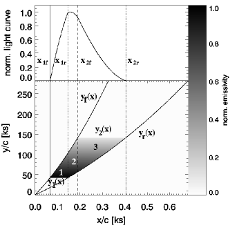
In order to compute the light curve emitted by the horn–shaped region (Fig. 5), we note that significant emission occurs only after the actual interaction of the shells starts and that this emission only lasts until the internal shocks reach the edge of the merged shell which terminates the shell interaction. Hence, one needs to calculate only the light curve produced by a segment of the horn–shaped region defined by two times, $T_{1}$ (start of the interaction) and $T_{2}$ (termination of the interaction). We assume an emissivity distribution in the source frame of the form

$$\begin{array}[]{rl}j(z,T)=&j_{0}\left[1+\displaystyle{\frac{T^{\theta}-T_{1}^{\theta}}{T_{2}^{\theta}-T_{1}^{\theta}}}(\eta-1)\right]\times\\[14.22636pt] &S(T;T_{1},T_{2})S\left[z;z_{\rm b}(T),z_{\rm f}(T)\right]\,,\end{array}$$ (24)

where $\theta$ is a power law index describing the temporal change of the emissivity, and $\eta$ is the ratio of the final $j(T_{2})$ and the initial $j_{0}\equiv j(T_{1})$ emissivities. The interval function $S(T;T_{1},T_{2})$ ((11) appearing in the above expression will be dropped in the following discussion.

Substituting (4) and (5) into (24), the emissivity in the observer frame ($xy$–coordinates) becomes

$$j(x,y)=\displaystyle{\frac{j_{0}}{T_{2}^{\theta}-T_{1}^{\theta}}}\left[T_{2}^{\theta}-\eta T_{1}^{\theta}+\displaystyle{\frac{(x+y)^{\theta}}{(\sqrt{2}c)^{\theta}}}(\eta-1)\right]\,.$$ (25)

The segment of the horn-shaped region is bound by the two parabolae $y_{\rm f}(x)$ and $y_{\rm b}(x)$ in $x$–direction (see § 4.2), and by the following two straight lines in $y$–direction (Fig. 5),

$$y_{1}(x)=\sqrt{2}cT_{1}-x\,,$$ (26)

$$y_{2}(x)=\sqrt{2}cT_{2}-x\,.$$ (27)

The light curve $I(x)$ at a given $x$–coordinate is obtained by integrating the emissivity distribution at that $x$–coordinate in $y$–direction. According to our model the integration limits depend on the value of the $x$–coordinate, and three regions can be distinguished (Fig. 5). In region 1 ($x_{1{\rm f}}\leq x\leq x_{1{\rm b}}$) the integration extends from $y_{1}(x)$ to $y_{\rm f}(x)$, in region 2 ($x_{1{\rm b}}<x\leq x_{2{\rm f}}$) from $y_{\rm b}(x)$ to $y_{\rm f}(x)$, and in region 3 ($x_{2{\rm f}}<x\leq x_{2{\rm b}}$) from $y_{\rm b}(x)$ to $y_{2}(x)$ (see Fig. 5). The coordinates $x_{1{\rm b}}$, $x_{1{\rm f}}$, $x_{2{\rm b}}$, and $x_{2{\rm f}}$ are given by

$$x_{1{\rm b}}=\displaystyle{\frac{\sqrt{2}cT_{1}}{2\Gamma_{\rm b}^{2}}}\displaystyle{\frac{1}{1+\sqrt{1+K_{\rm b}T_{1}/T_{e}}}}\,,$$ (28)

$$x_{1{\rm f}}=\displaystyle{\frac{\sqrt{2}cT_{1}}{2\Gamma_{\rm f}^{2}}}\displaystyle{\frac{1}{1+\sqrt{1+K_{\rm f}T_{1}/T_{e}}}}\,,$$ (29)

$$x_{2{\rm b}}=\displaystyle{\frac{\sqrt{2}cT_{2}}{2\Gamma_{\rm b}^{2}}}\displaystyle{\frac{1}{1+\sqrt{1+K_{\rm b}T_{2}/T_{e}}}}\,,$$ (30)

$$x_{2{\rm f}}=\displaystyle{\frac{\sqrt{2}cT_{2}}{2\Gamma_{\rm f}^{2}}}\displaystyle{\frac{1}{1+\sqrt{1+K_{\rm f}T_{2}/T_{e}}}}\,,$$ (31)

where we assume $x_{1{\rm b}}<x_{2{\rm f}}$ (see next section for discussion). Thus, $x_{1{\rm f}}<x_{1{\rm b}}<x_{2{\rm f}}<x_{2{\rm b}}$. Defining two auxiliary functions

$$g(\xi,K,\Gamma)=4\Gamma^{2}(\Gamma^{2}K\xi^{2}+\xi)\,,$$ (32)

and

$$\begin{array}[]{l}H(A,B,\tau_{1},\tau_{2},\theta,\eta)=\displaystyle{\frac{1}{\tau_{2}^{\theta}-\tau_{1}^{\theta}}}\times\\[14.22636pt] \,\,\,\,\,\,\,\,\left[(\tau_{2}^{\theta}-\eta\tau_{1}^{\theta})(B-A)+\displaystyle{\frac{(\eta-1)(B^{\theta+1}-A^{\theta+1})}{\theta+1}}\right]\end{array}$$ (33)

allows us to write the light curve of a segment of the horn-shaped region in a very compact way,

$$\begin{array}[]{l}I(x)=j_{0}\sqrt{2}cT_{\rm e}\times\\[14.22636pt] \,\,\,\,\,\,\,\,\left\{\begin{array}[]{ll}H\left[\displaystyle{\frac{T_{1}}{T_{\rm e}}},g_{\rm f}(x),\displaystyle{\frac{T_{1}}{T_{\rm e}}},\displaystyle{\frac{T_{2}}{T_{\rm e}}},\theta,\eta\right]&{\rm if}\,x_{1{\rm f}}\leq x\leq x_{1{\rm b}}\\[11.38109pt] H\left[g_{\rm b}(x),g_{\rm f}(x),\displaystyle{\frac{T_{1}}{T_{\rm e}}},\displaystyle{\frac{T_{2}}{T_{\rm e}}},\theta,\eta\right]&{\rm if}\,x_{1{\rm b}}<x\leq x_{2{\rm f}}\\[11.38109pt] H\left[g_{\rm b}(x),\displaystyle{\frac{T_{2}}{T_{\rm e}}},\displaystyle{\frac{T_{1}}{T_{\rm e}}},\displaystyle{\frac{T_{2}}{T_{\rm e}}},\theta,\eta\right]&{\rm if}\,x_{2{\rm f}}<x\leq x_{2{\rm b}}\end{array}\right.\end{array}$$ (34)

where $g_{\rm f}(x)$ and $g_{\rm b}(x)$ are given by

$$g_{\rm f}(x)\equiv g\left(\displaystyle{\frac{x}{\sqrt{2}cT_{\rm e}}},K_{\rm f},\Gamma_{\rm f}\right)\,,$$

$$g_{\rm b}(x)\equiv g\left(\displaystyle{\frac{x}{\sqrt{2}cT_{\rm e}}},K_{\rm b},\Gamma_{\rm b}\right)\,.$$

The upper panel of Fig. 5 shows an example of a light curve computed from Eq. (34) for $\Gamma_{\rm b}=8$, $K_{\rm b}=4$, $\Gamma_{\rm f}=12$, $K_{\rm f}=3$, $T_{1}=30$ ks, $T_{2}=100$ ks, $T_{\rm e}=200$ ks, $\eta=0.1$, and $\theta=1$.

4.4 Two-phase flare model

As discussed in § 2 and by MAMB04, the interaction of two shells consists of three basic phases: a fast rise of the pressure, a slow pressure decrease while the internal shocks propagate through the shells, and finally the acceleration of the front shock as it breaks out of the slower shell. In our analytic model we simplify the situation by assuming only two phases, and hence call it a two-phase flare model. For the first phase ($0\leq T\leq T_{\rm i}$) we assume that the initial and final values of the emissivity are $j_{0}$ and $\eta_{1}j_{0}$, respectively. In the second phase ($T_{\rm i}\leq T\leq T_{\rm e}$) the emissivity is assumed to abruptly jump to a value $\eta_{2}j_{0}$, and then to decrease to zero. The abrupt jump is motivated by the fact that when the forward shock, created by the interaction of the shells, is about to break out of the slower shell, it encounters the reverse shock produced by the pre–collision hydrodynamic evolution of its leading edge. The interaction of these two shocks causes a fast rise both of the pressure and the density, i.e., $\eta_{2}>\eta_{1}$.

Figure 6: Two–phase flare model with $\Gamma_{\rm b}=5.5$, $K_{\rm b}=1.1$, $\Gamma_{\rm f}=6$, $K_{\rm f}=4$, $T_{\rm i}=50$ ks, $T_{\rm e}=100$ ks, $\theta_{1}=1$, $\theta_{2}=1$ and $\eta_{1}=100$, and $\eta_{2}=300$. The upper panel shows the normalized light curve, and the lower one the emissivity. The vertical lines denote the coordinates $x_{1}$ (solid), $x_{2}$ (dotted), $x_{3}$ (dashed), and $x_{4}$ (dot-dashed line) which divide the emissivity distribution into four distinct regions labeled by numbers 1 to 4. The white thick horizontal line separates the two phases of the temporal evolution of the emissivity.

Figure 7: Same as Fig. 6, but for $\eta_{2}=101$.

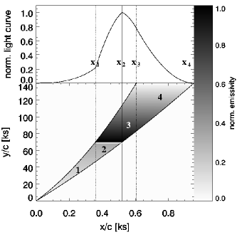
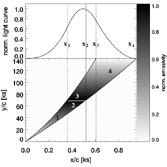
The light curve ${\cal I}(x)$ of the two–phase flare model is then computed as follows: we assume that the emissivity $j(T)$ has the form

$$j(T)=j_{0}\left\{\begin{array}[]{ll}1+\displaystyle{\frac{T^{\theta_{1}}}{T_{\rm i}^{\theta_{1}}}}(\eta_{1}-1)&{\rm if}\,0\leq T\leq T_{\rm i}\\[14.22636pt] \eta_{2}\left[1-\displaystyle{\frac{T^{\theta_{2}}-T_{\rm i}^{\theta_{2}}}{T_{\rm e}^{\theta_{2}}-T_{\rm i}^{\theta_{2}}}}\right]&{\rm if}\,T_{\rm i}\leq T\leq T_{\rm e}\end{array}\right.\,,$$ (35)

and that the light curve in both phases (i.e., in both sub–segments of the horn-shaped emission region; see (Fig. 6) has the form of the light curve $I(x)$ (34) with common parameters $\Gamma_{\rm b}$, $K_{\rm b}$, $\Gamma_{\rm f}$, and $K_{\rm f}$, but with the sub–segment specific parameters according to the following substitutions:

• segment  1:  $j_{0}$, $T_{1}\rightarrow 0$, $T_{2}\rightarrow T_{\rm i}$, $\theta\rightarrow\theta_{1}$, $\eta\rightarrow\eta_{1}$

• segment 2:  $j_{0}\rightarrow\eta_{2}j_{0}$, $T_{1}\rightarrow T_{\rm i}$, $T_{2}\rightarrow T_{\rm e}$, $\theta\rightarrow\theta_{2}$, $\eta\rightarrow 0$   .

In order to obtain the light curve ${\cal I}(x)$ of the two–phase flare model (again by integrating the emissivity distribution at each $x$–coordinate in $y$–direction) the horn–shaped emissivity region is divided into four distinct regions defined by (Fig. 6)

$$x_{1} = \displaystyle{\frac{\sqrt{2}cT_{\rm i}}{2\Gamma_{\rm f}^{2}}}\displaystyle{\frac{1}{1+\sqrt{1+K_{\rm f}T_{\rm i}/T_{\rm e}}}}\,,$$ (36)

$$x_{2} = \displaystyle{\frac{\sqrt{2}cT_{\rm i}}{2\Gamma_{\rm b}^{2}}}\displaystyle{\frac{1}{1+\sqrt{1+K_{\rm b}T_{\rm i}/T_{\rm e}}}}\,,$$ (37)

$$x_{3} = \displaystyle{\frac{\sqrt{2}cT_{\rm e}}{2\Gamma_{\rm f}^{2}}}\displaystyle{\frac{1}{1+\sqrt{1+K_{\rm f}}}}\,,$$ (38)

$$x_{4} = \displaystyle{\frac{\sqrt{2}cT_{\rm e}}{2\Gamma_{\rm b}^{2}}}\displaystyle{\frac{1}{1+\sqrt{1+K_{\rm b}}}}\,.$$ (39)

Then, using the auxiliary functions $H$, $g_{\rm b}$ and $g_{\rm f}$ defined in § 4.3, one can write the light curve of the two–phase model in the form

$$\begin{array}[]{l}{\cal I}(x)=j_{0}\sqrt{2}cT_{\rm e}\times\\[5.69054pt] \,\,\,\,\,\,\,\,\left\{\begin{array}[]{ll}H\left[g_{\rm b}(x),g_{\rm f}(x),0,\displaystyle{\frac{T_{\rm i}}{T_{\rm e}}},\theta_{1},\eta_{1}\right]&{\rm if}\,\,0\leq x\leq x_{1}\\[28.45274pt] \begin{array}[]{l}H\left[g_{\rm b}(x),\displaystyle{\frac{T_{\rm i}}{T_{\rm e}}},0,\displaystyle{\frac{T_{\rm i}}{T_{\rm e}}},\theta_{1},\eta_{1}\right]+\\[11.38109pt] \eta_{2}H\left[\displaystyle{\frac{T_{\rm i}}{T_{\rm e}}},g_{\rm f}(x),\displaystyle{\frac{T_{\rm i}}{T_{\rm e}}},1,\theta_{2},0\right]\end{array}&{\rm if}\,\,x_{1}<x\leq x_{2}\\[42.67912pt] \eta_{2}H\left[g_{\rm b}(x),g_{\rm f}(x),\displaystyle{\frac{T_{\rm i}}{T_{\rm e}}},1,\theta_{2},0\right]&{\rm if}\,\,x_{2}<x\leq x_{3}\\[28.45274pt] \eta_{2}H\left[g_{\rm b}(x),1,\displaystyle{\frac{T_{\rm i}}{T_{\rm e}}},1,\theta_{2},0\right]&{\rm if}\,\,x_{3}<x\leq x_{4}\end{array}\right.\end{array}$$ (40)

Figs. 6 and 7 show two examples of analytic two–phase light curves, which only differ in the value of $\eta_{2}$ with $\eta_{2}=300$ in Fig. 6 and $\eta_{2}=101$ in Fig. 7, respectively.

4.5 Normalized two-phase model

As pointed out in § 4.1, all observed time scales are functions of $T/\Gamma^{2}$, where $T$ is a typical time scale in the source frame, and $\Gamma$ is a typical Lorentz factor at which the emitting region is moving. In order to make our model “aware” of this, we introduce the normalized coordinate

$$\xi\equiv\displaystyle{\frac{x}{x_{4}}}=\displaystyle{\frac{2\Gamma_{\rm b}^{2}}{\sqrt{2}cT_{\rm e}}}(1+\sqrt{1+K_{\rm b}})\,,$$ (41)

and define

$$\gamma_{\rm b}\equiv\displaystyle{\frac{\Gamma_{\rm b}}{\Gamma_{\rm f}}}$$ (42)

and

$$t_{\rm i}\equiv\displaystyle{\frac{T_{\rm i}}{T_{\rm e}}}\,.$$ (43)

Thereby we can specify a normalized (both in intensity and in time) flare model

$${\cal F}(\xi)={\cal F}_{0}\left\{\begin{array}[]{lr}H[h_{\rm b}(\xi),h_{\rm f}(\xi),0,t_{\rm i},\theta_{1},\eta_{1}]&{\rm if\,}0\leq\xi\leq\xi_{1}\\[11.38109pt] \begin{array}[]{l}H[h_{\rm b}(\xi),t_{\rm i},0,t_{\rm i},\theta_{1},\eta_{1}]+\\[5.69054pt] \eta_{2}H[t_{\rm i},h_{\rm f}(\xi),t_{\rm i},1,\theta_{2},0]\end{array}&{\rm if\,}\xi_{1}<\xi\leq\xi_{2}\\[11.38109pt] \eta_{2}H[h_{\rm b}(\xi),h_{\rm f}(\xi),t_{\rm i},1,\theta_{2},0]&{\rm if\,}\xi_{2}<\xi\leq\xi_{3}\\[11.38109pt] \eta_{2}H[h_{\rm b}(\xi),1,t_{\rm i},1,\theta_{2},0]&{\rm if\,}\xi_{3}<\xi\leq 1\end{array}\right.$$ (44)

where the constant ${\cal F}_{0}$ is chosen such that the maximum value of ${\cal F}(\xi)$ is $1$. The points $\xi_{i}$, $i=1,2,3$ are given by

$$\xi_{1}\equiv\gamma_{\rm b}^{2}t_{\rm i}\displaystyle{\frac{1+\sqrt{1+K_{\rm b}}}{1+\sqrt{1+K_{\rm f}t_{\rm i}}}}\,,$$ (45)

$$\xi_{2}\equiv t_{\rm i}\displaystyle{\frac{1+\sqrt{1+K_{\rm b}}}{1+\sqrt{1+K_{\rm b}t_{\rm i}}}}\,,$$ (46)

$$\xi_{3}\equiv\gamma_{\rm b}^{2}\displaystyle{\frac{1+\sqrt{1+K_{\rm b}}}{1+\sqrt{1+K_{\rm f}}}}\,,$$ (47)

and the auxiliary functions $h_{\rm b}(\xi)$ and $h_{\rm f}(\xi)$ are obtained from $g_{\rm b}(x)$ and $g_{\rm f}(x)$, respectively:

$$h_{\rm b}(\xi)=\displaystyle{\frac{K_{\rm b}\xi^{2}}{(1+\sqrt{1+K_{\rm b}})^{2}}}+\displaystyle{\frac{2\xi}{1+\sqrt{1+K_{\rm b}}}}\,,$$ (48)

and

$$h_{\rm f}(\xi)=\displaystyle{\frac{K_{\rm f}\xi^{2}}{\gamma_{\rm b}^{4}(1+\sqrt{1+K_{\rm b}})^{2}}}+\displaystyle{\frac{2\xi}{\gamma_{\rm b}^{2}(1+\sqrt{1+K_{\rm b}})}}\,.$$ (49)

The normalized two–phase model has the advantage that the absolute intensity is no longer a parameter, and that it has embedded the intrinsic degeneracies of $T/\Gamma^{2}$ which must be present in the model due to the relativistic time contraction. Indeed, the normalized two–phase model uses two parameter less in order to fit the light curves. Therefore, we find that the fitting procedure is always convergent.

5 Fits of the analytic model to synthetic light curves

The final goal of our analytic modeling of the light curve of a flare is to extract unobservable physical parameters of the emitting region. As a first step, we have validated our analytic model by comparing the parameters extracted from fits of synthetic light curves (computed from our hydrodynamic models) to the parameters that we can directly obtain from the same hydrodynamic models. The second step will be to apply our validated analytic model to real observations, which is beyond the scope of this paper.

Table 3 shows the results of the fit of the analytic model to the soft ($0.1$-$1$ keV) light curves of all seven models. First, we observe that the ratios $\gamma_{\rm b}^{\rm sim}\equiv\Gamma_{\rm b}^{\rm sim}/\Gamma_{\rm f}^{\rm sim}$) and $\gamma_{\rm b}\equiv\Gamma_{\rm b}/\Gamma_{\rm f}$ are very similar, but not exactly the same, i.e., there exists a correlation between the values obtained from the simulations and the fit. Second, the small values of the parameter $K_{\rm b}$ indicate a lack of acceleration of the reverse shock, i.e., the reverse shock moves at almost constant velocity until it breaks out of the faster shell. This is clearly seen in Fig. 9, where the trajectory (world–line) of the reverse shock (full thick line) is a straight line between points $a$ and $d$, which correspond to the start of the interaction and the time and place where the reverse shock breaks out of the faster shell, respectively. Third, the values of the parameter $K_{\rm f}$ imply that the forward shock accelerates, though its Lorentz factor does not increase by more than about $30\%$ (model S10-F14). From the simulations, we see that the forward shock (dashed thick line in Fig. 9) moves at approximately constant velocity between points $a$ and $b$ the latter point corresponding to the time and place where the forward shock catches up with the reverse shock emerging from the leading edge of the slower shell – see Sec. 4.4). Afterwards, beyond point $b$, the forward shock speeds up, because it breaks out of the slower shell. Therefore, in the time interval between the formation of the forward shock and the time when the emissivity associated to it ceases to contribute to the light curve, there is a net acceleration of this shock. This is also properly captured by our analytic model. Fourth, on the one hand, considering the models having the same inertial mass of the slower shell (rows 1–4 in Tab. 3) the time $t_{\rm b}$ necessary for the forward shock to break out of that shell, relative to the total flare duration in the laboratory frame, decreases with increasing inertial mass of the faster shell. On the other hand, we find a similar correlation considering those models where the inertial mass of the faster shell is fixed (rows 1, 5, 6 and 7), i.e., $t_{\rm b}$ is decreasing as the inertial mass of the slower shell increases (see Sec. 7.1).

sim.	$\gamma_{\rm b}^{\rm sim}$	$\gamma_{\rm b}$	$K_{\rm b}$	$K_{\rm f}$	$t_{\rm b}$
S10-F10	$0.943$	$0.832$	$3.4\times 10^{-6}$	$1.07$	$0.429$
S10-F07	$0.940$	$0.867$	$1.2\times 10^{-4}$	$1.68$	$0.434$
S10-F05	$0.937$	$0.861$	$2.5\times 10^{-4}$	$1.39$	$0.445$
S10-F14	$0.944$	$0.855$	$6.4\times 10^{-4}$	$2.35$	$0.414$
S07-F10	$0.946$	$0.913$	$7.2\times 10^{-5}$	$1.40$	$0.567$
S05-F10	$0.948$	$0.887$	$1.1\times 10^{-4}$	$1.95$	$0.579$
S14-F10	$0.941$	$0.839$	$1.09\times 10^{-4}$	$1.34$	$0.415$

Table 3: Results of the fit of the normalized analytic model to the soft ($0.1$-$1$ keV) light curves of all simulated models. $\gamma_{\rm b}^{\rm sim}$ is the ratio $\Gamma_{\rm b}^{\rm sim}/\Gamma_{\rm f}^{\rm sim}$ computed from the models (see Tab. 1). The rest of the columns provide the other parameters obtained by fitting the normalized analytic model.

Figure 8: Soft light curve of model S05-F10 (dotted line), and the best fit of the normalized analytic model (full line).

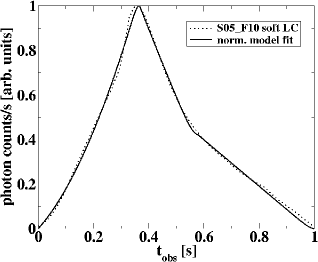
6 Space time emissivity distribution

Figure 9: The distribution of the emissivity in the observer frame in $xy$–coordinates in the soft photon band (lower panel), and the corresponding soft light curve (upper panel) for model S05-F10. The grey contours show the emissivity distribution on a linear scale. The full, dotted, dashed, and dot–dashed lines denote positions of the back edge of the slower shell, the front edge of the slower shell, the back edge of the faster shell, and the front edge of the faster shell, respectively. The full thick and dashed thick lines show the trajectories of the reverse and forward shock, respectively.

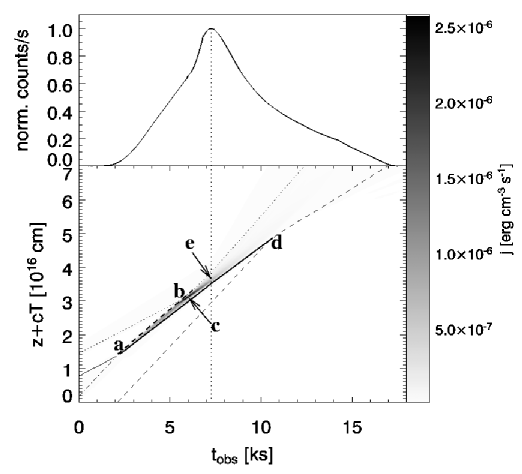
From Fig. 9, which shows the soft light curve (upper panel) and a grey contour plot of the emissivity distribution in the observer frame using the $xy$–coordinates (lower panel) for model S05-F10, one sees that the emissivity distribution has the shape expected from the analytic model, i.e., a horn–like shape starting at point $a$ where the internal shocks form. The region then widens as the shocks propagate through the shells. The bulk of the radiation is produced relatively early in the evolution (up to point $c$ in Fig. 9, which corresponds to the moment of maximum emissivity), i.e., the subsequent formation of rarefaction waves does not have any influence on the observed light curve (see, however, §  7.1 for a discussion of the possible influence on later collisions). We point out that there might be a difference between the time (in the observer frame) when the light curve has a maximum (point $e$), and the point when the emissivity has a maximum (point $c$). This difference arises because the total observed intensity at a given time is the result of an integration of the emissivity over the emitting region. Thus, the maximum observed intensity can result from a region where the emissivity is not maximal, but whose emitting volume is sufficiently large. In case of model S05-F10 (Fig. 9) the maximal observed intensity is delayed with respect to the maximum of the emissivity. This influences the shape of the light curve, because prior to the maximum, at $t_{\rm obs}\approx 6$ ks, we see a kink in the light curve where its slope steepens. When the emissivity maximum (in the observer frame) happens close to, or even after the intensity maximum, no such kink will appear (see Figs. 6 and 7, which illustrate precisely these two cases).

7 Discussion

We have performed a detailed study of two–shell collisions in the framework of the internal shock model using relativistic hydrodynamic simulations. The non–thermal radiation emitted by shocked plasma is consistently coupled to the hydrodynamics (including the radiation back–reaction on the dynamics) in our numerical scheme. Our findings can be applied to extract physical parameters of the emitting regions of blazar flares. However, the method of extracting physical parameters out of synchrotron light curves might as well be applied to other astrophysical scenarios where internal shocks occur (e.g., gamma–ray bursts).

7.1 Hydrodynamic evolution of the shell interaction

The properties of the interaction common to all our models are the existence of three main phases of evolution (Figs. 1 and 2): (i) the pre–collision phase where the front edges of the shells pile up matter from the external medium and are heated due to their interaction with the latter, (ii) the collision phase where the internal shocks form and propagate through the shells, and (iii) the post–collision or rarefaction phase where the reverse shock has broken out of the faster shell creating rarefaction waves which expand the merged shell and cause its structure to become multi–peaked. Although this multi–peaked structure does not have any influence on the observed flare, one has to bear in mind that any shell colliding subsequently with the merged shell will encounter a non–uniform structure, which will probably cause the forward shock, originating after the new shell collision, to undergo a much more complicated set of non–linear wave interactions than in the case of initially uniform shells. This will yield a more complex light curve profile. We also point out that the insensitivity of the light curve profiles to the large rest–mass density and specific energy variations in the merged shell, may probably prevent one from extracting from any simple one-zone model accurate information about these hydrodynamic variables from fits of the observed flare light curves. This lack of sensitivity to the rest–mass density profile comes from the fact that most of the steep density gradients in the merged shell are either weak shocks or no shocks at all. Hence, no significant emission can be originated in such steep density variations and the resulting light curve remains uninfluenced. Furthermore, when assuming an approximately uniform proportionality between the rest–mass energy and the magnetic field energy (i.e., the ratio $B^{2}/\rho$ being approximately uniform) accurate values of the magnetic field strength are hardly to be inferred from a flare light curve, too.

We have also computed the instantaneous efficiency of conversion of kinetic energy into internal energy of the fluid. As can be seen from Fig. 3, the efficiency rises initially, then remains constant for a period of time during which the front edge of the faster shell propagates through the rarefaction caused by the back edge of the slower shell, and then rises again when the internal shocks form. The efficiency during the period when most of the radiation is observed is larger than the analytically predicted value. Afterwards, it decreases and reaches the analytically predicted values.

For a fixed inertial mass of the slower shell, the Lorentz factor of the reverse and forward shocks grows as the inertial mass of the faster shell increases. Conversely, fixing the inertial mass of the faster shell, the Lorentz factor of the shocks decreases with increasing inertial mass of the slower shell. These correlations are expected, because increasing the inertial mass of the slower shell any incoming (faster) shell will supply less inertia (relative to that of the slower shell), i.e., the two internal shocks will propagate at smaller velocities. On the other hand, increasing the inertia of the faster shell will result in larger shock speeds, because the target shell does not decelerate the faster shell so efficiently.

The parameter $t_{\rm i}$, which is approximately the ratio of the time it takes the forward and reverse shocks to cross the slower and faster shell, respectively, depends on the inertial masses of the shells, too. We find that $t_{\rm i}$ decreases with increasing relative inertia of the faster shell (with respect to the slower one), because with increased inertia it is much easier for the forward shock to propagate through the slower shell and exiting from its front edge earlier than the reverse shock, which propagates into the heavier, faster shell.

7.2 Properties of the analytic model

As described in § 4, we have introduced the observer–xy coordinate system in order to simplify the relationship between the observed radiation and the space time evolution of the emissivity. By making assumptions about the properties of the emissivity distribution, we are able to construct an analytic model which depends on parameters of the internal shocks, namely the shock Lorentz factors and the shock propagation time scales. Our model can be applied to non–relativistic as well as ultra-relativistic shocks, and even allows for a (constant) acceleration of the shocks. For the moment, it does not take into account any spectral information, but we intend to improve our model in order to be able to interpret multi–frequency observations which may provide further restrictions on the physical parameters of the emitting regions. We have validated the analytic model by comparing its fitted parameters (using synthetic light curves) with their values obtained directly from the simulations which provide the synthetic light curves.

7.3 Synthetic flares and the analytic model fitting

We find that all flares, once normalized, look qualitatively the same. This suggests that the exact shape of the flare depends mostly on the shock Lorentz factors and shock propagation time scales while it is rather insensitive to the distribution of the rest–mass density or specific energy within the emitting region (see § 7.1). We have fitted the analytic model (using a simple genetic algorithm) to synthetic light curves and have achieved satisfactory results. The deviations in the parameters between the simulation and the fit (Tab. 3) are due to the simplifications of the analytic model, e.g., the assumption that the emissivity is constant between internal shocks (this is not exactly the case, as can be seen in Fig. 9). However, the general shape of the emissivity distribution (Fig. 9) does match our assumptions. This implies that one might fit the model parameters using the observed X-ray light curves of blazar flares (e.g., Mrk 421) and recover shock parameters, like e.g., the ratio of Lorentz factors between the reverse and forward shock, the propagation time scales through the shells, and the kinematic evolution (acceleration) of the shock fronts. However, here the quality of the observations might play a crucial role, since the analytic model is very sensitive to changes in the flare shape, as can be seen from Figs.  6 and 7.

We have produced synthetic observations in soft and hard energy bands (Fig. 4). A correlation between the peak photon counts and the initial rest mass density of the shells has been found. Currently, we are performing a more detailed parameter study aiming to confirm this suspected correlation for cases of different shell Lorentz factors and densities. The peak in the hard band is observed several hundreds of seconds before the one in the soft band. However, the exact value of the lag between the hard and soft peaks will be different in the case of varying shock strengths and velocities (which strongly depend on the shell properties). Additionally, the possible acceleration of particles inside the emitting region is not included in our model. Instead, particles are injected into the plasma with a given energy distribution, as acceleration timescales are expected to be shorter than the dynamical timescale. Note, however, that acceleration may be the origin of some of the features (sign of the delay) observed in temporal evolution of these sources (e.g., Kirk, Rieger & Mastichiadis  1998).

Observationally, the lags between the peaks in the soft and hard bands are still a matter of controversial debate. The emission of the soft X-rays can be well correlated with that of the hard X-rays lagging it by 3$-$4 ks (Takahashi et al. 1996, 2000, Zhang et al. 1999, Malizia et al. 2000, Kataoka et al. 2000, Fossati et al. 2000). However, significant lags of both signs were detected from several flares (Tanihata et al. 2001). The lags between the soft and hard peaks may depend on the assumed value of the parameter $\alpha_{B}=(B^{2}/8\pi)/(\rho\varepsilon)$ which sets the strength of the magnetic field in the emitting region. As in MAMB04 this parameter has been chosen such that the field strength resulting from the hydrodynamic evolution yields values of $\sim 0.1$ G (the value of $\alpha_{B}$ is the same for all our models). This field strength lies in the ballpark of the values inferred from detailed fits of SED curves of several sources (see, e.g., Tanihata et al.  2001). We point out that even for the same source there is no consensus on the exact value of the magnetic field strength. For example, Tanihata et al.  (2001) report $B\sim 0.14\,$G for PKS 2155-304, while is inferred $B\sim 1.5\,$G from Chiappetti et al.  (1999) for the same source (taking the Doppler factor to be $\delta=28$; Tanihata et al. 2001).

Observations of PKS 2155-304 Edelson et al. (2001) using $XMM-Newton$suggest that previous claims of soft lags with time scales of $\sim$ hours might be an artifact of the periodic interruptions of the low–Earth orbits of the satellites every $\sim 1.6$ hours. This claim was questioned by Zhang et al. (2004) who show that, although periodic gaps introduce larger uncertainties than present in evenly sampled data, lags on time scales of hours cannot be the result of periodic gaps. Large flares with time scales of $\sim 1$ day were detected with temporal lags of less than 1.5 hours between X-ray and TeV energies (for Mrk 421 see Takahashi et al. 2000).

Recently, very detailed studies of Mrk 421 with $XMM-Newton$(Brinkmann et al. 2003, 2005; Ravasio et al.  2004) clearly show that the source exhibits stronger variability when it is brighter, that the cross correlation function appears to change “continuously”, and depending on the length of the observing window and the actual activity state of the source they find periods with positive, negative or no lags, but also periods of weak correlations between the soft and hard energy bands. Here we propose that the apparent sign of the lags is the result of the particular arrangement of a number of emitting regions, i.e., the resulting spectral properties will depend strongly on the time scales of their emission, as well as their distances and relative velocities.