Infrared Surface Brightness Distances to Cepheids: a comparison of Bayesian and linear-bisector calculations

Abstract

We have compared the results of Bayesian statistical calculations and linear-bisector calculations for obtaining Cepheid distances and radii by the infrared surface brightness method. We analyzed a set of 38 Cepheids using a Bayesian Markov Chain Monte Carlo method that had been recently studied with a linear-bisector method. The distances obtained by the two techniques agree to $1.5\%\pm 0.6\%$ with the Bayesian distances being larger. The radii agree to $1.1\%\pm 0.7\%$ with the Bayesian determinations again being larger. We interpret this result as demonstrating that the two methods yield the same distances and radii. This implies that the short distance to the LMC found in recent linear-bisector studies of Cepheids is not caused by deficiencies in the mathematical treatment. However, the computed uncertainties in distance and radius for our dataset are larger in the Bayesian calculation by factors of 1.4–6.7. We give reasons to favor the Bayesian computations of the uncertainties. The larger uncertainties can have a significant impact upon interpretation of Cepheid distances and radii obtained from the infrared surface brightness method.

1 Introduction

The infrared surface brightness technique is a powerful method for determining distances to Cepheid variables (Welch 1994, Fouqué & Gieren 1997). It is independent of other astrophysical distance scales, nearly independent of errors in reddening, and may be applied to arbitrarily-chosen, individual Cepheids at great distances. However, the implementation of the infrared surface brightness technique and its predecessor, the visual surface brightness method, have been criticized as not mathematically rigorous in their solutions to the surface brightness equations (Laney & Stobie 1995, Barnes & Jefferys 1999). This leads to the possibility that the distances, radii, and their uncertainties may be erroneous.

This is of current interest as Storm et al. (2004) have found a short distance to the LMC based on a linear-bisector analysis of six Cepheids in the LMC cluster NGC1866. They also found a slope to the LMC Cepheid period-luminosity relation that is substantially different than found in the OGLE magnitudes (Udalski et al. 1999). It is important to determine if their results are affected by the mathematical method used in the surface brightness analysis.

To address the larger issue Barnes et al. (2003) developed a Bayesian Markov Chain Monte Carlo (MCMC) solution to the surface brightness equations that is mathematically rigorous. In the current paper we do a direct comparison for a significant sample of Cepheids between the Bayesian MCMC solution and recent linear-bisector calculations (Storm et al. 2004, Gieren et al. 2005) to explore possible differences. The two methods used identical data, identical surface brightness equations and identical physical constants to ensure that only the mathematical approaches were compared.

In the next section we introduce the surface brightness method for determining distances and radii and present the background of the infrared surface brightness method. We then discuss the data that are used for the two calculations. We review the linear-bisector calculations and the Bayesian MCMC calculations. In section 6 we compare the results of the two methods for 38 Galactic Cepheids. Finally we discuss the importance of the agreement and the differences that we find.

2 The Surface Brightness Method

2.1 The surface brightness equations

The infrared surface brightness method is a modification of the visual surface brightness technique developed by Barnes et al. (1977) and thus shares the same computational algorithm. Because solution of the equations is the important issue, we introduce the equations in some detail. Useful discussions of previous work have been given by Gieren, Barnes & Moffett (1993), Fouqué & Gieren (1997), Nordgren et al. (2002), Fouqué, Storm, & Gieren (2003), and Barnes et al. (2003).

Barnes & Evans (1976) and Barnes, Evans, & Parsons (1976) defined a visual surface brightness parameter $F_{V}$ as

$$F_{V}=4.2207-0.1V{\rm{}_{0}}-0.5\log\phi$$ (1)

and also as,

$$F_{V}=\log{T_{e}}+0.1BC,$$ (2)

where $V{\rm{}_{0}}$ is the stellar visual magnitude corrected for interstellar extinction, $\phi$ is the stellar angular diameter expressed in milliarcseconds, $T_{e}$ is the effective temperature and $BC$ is the bolometric correction.

They demonstrated that $F_{V}$ is well correlated with Johnson color index $(V-R){\rm{}_{0}}$ for a very wide range of stellar types.

$$F_{V}=A+B\left(V-R\right){\rm{}_{0}}$$ (3)

equation (3) is called the visual surface brightness relation.

These relations led Barnes et al. (1977) to infer a distance scale for Cepheids as follows. At each time $t$ in the pulsation of the Cepheid, equations (1) and (3) may be combined to obtain the angular diameter variation of the star, $\phi(t)$,

$$4.2207-0.1V{\rm{}_{0}}(t)-0.5\log\phi(t)=A+B\left(V-R\right){\rm{}_{0}}(t)$$ (4)

In addition we infer the Cepheid’s linear radius variation ${\Delta}R(t)$ about the mean radius from an integration of the radial velocity curve, $V_{r}(t)$,

$${\Delta}R(t)=-\int{p\left(V_{r}(t)-{V_{\gamma}}\right)dt}$$ (5)

where the factor $-p$ converts observed radial velocity to the star’s pulsational velocity and $V_{\gamma}$ is the center-of-mass radial velocity of the star. Integration of the discrete radial velocity data requires that the velocity variation be appropriately modeled.

Substituting into equation (4), the relation among mean angular diameter $\phi_{0}$, linear diameter $\Delta R(t)$, and distance $r$, we obtain

$$4.2207-0.1V{\rm{}_{0}}(t)-0.5\log(\phi_{0}+2000\Delta R(t)/r)=A+B\left(V-R\right){\rm{}_{0}}(t).$$ (6)

where $\phi_{0}$ is in milliarcseconds, $r$ is in parsecs, and $\Delta R(t)$ is in AU. The factor $2000$ converts radius to diameter and arcseconds to milliarcseconds.

Until very recently direct solution to equation (6) for distance and diameter has proved daunting. Various methods have been tried, but for reasons given by Barnes & Jefferys (1999), none of the methods is rigorous.

Barnes et al. (1977), Gieren et al. (1993, 1997) and Welch (1994) simplified the problem by solving equation (4) for $\phi(t)$, solving equation (5) for $\Delta R(t)$ and then solving for $r$ and $\phi_{0}$ using ordinary least-squares solution on equation (7) taking $\Delta R(t)$ as the independent variable.

$$\Delta R(t)=r(\phi_{0}+\phi(t))/2000$$ (7)

However, the least-squares calculations do not properly treat the errors-in-variables problem that arises from uncertainty in both $\Delta R(t)$ and $\phi(t)$. The best that can be done using least-squares is the linear-bisector solution. Isobe et al. (1990) showed that linear-bisector performs better than other least-squares solutions when the problem is symmetric in the variables, as is the case here. Storm et al. (2004) adopted the linear-bisector method.

Following Balona (1977), Laney & Stobie (1995) linearized equation (6) and applied a maximum-likelihood calculation to its solution. They used an iterative maximum-likelihood method to solve for the larger amplitude Cepheids for which the linearization is invalid. Their calculation addresses the errors-in-variables problem. However, results from the maximum-likelihood method can be quite sensitive to accurate knowledge of the uncertainties in the data, as discussed by Gieren et al. 1997.

All the above methods require that the observed radial velocities be modeled in order to do the integration of equation (5). This creates a model selection problem. Most researchers choose a Fourier series to fit the radial velocities, but the number of terms to include in the series is subjectively chosen.

Finally, whether least-squares or maximum-likelihood, the above calculations fail to treat properly the propagation of observational error through the radial velocity integral, equation (5). Balona (1977) introduced a widely used approximation to the error in $\Delta R(t)$ based on the uncertainty in the radial velocity data and on the assumption that the radial velocity data are equally spaced in pulsation phase, which is rarely true.

It was to address these issues that the Bayesian MCMC method was developed by Barnes et al. (2003). Their calculation correctly solves the errors-in-variables problem, objectively selects the number of terms in the Fourier series fits, and correctly propagates the observational error through the radial velocity integration. Moreover, the Bayesian MCMC calculation does not demand that a particular Fourier series fit the data; rather, each Fourier series that is fit to the data has a particular posterior probability. That probability is used as a weight in determining the other quantities sought in the solution, i.e., distance, mean radius, etc.

A large number of calculations of variable star distances and radii by surface brightness methods are present in the literature. It is therefore of interest to determine the extent to which the above listed deficiencies affect those results. We will do this by comparing the linear-bisector calculations with Bayesian MCMC calculations.

2.2 The infrared surface brightness technique

Welch (1994) first showed that use of the infrared combination $K{\rm{}_{0}},(V-K){\rm{}_{0}}$ in place of $V{\rm{}_{0}},(V-R){\rm{}_{0}}$ in equation (6) has significant advantage in the precision of the distances and radii for Cepheids. He found an improvement by a factor of three in the distance uncertainty for the Cepheid U Sgr. Welch attributed the improved precision to several factors. First, the color index $(V-K){\rm{}_{0}}$ is as good an indicator of surface brightness as bluer color indices but much less sensitive to the complications of line blanketing and surface gravity. Second, the $K{\rm{}_{0}}$ magnitude lies on the Rayleigh-Jeans tail of the flux distribution and is therefore less affected by the surface brightness variation. It is obvious that a magnitude more sensitive to the radius variation that is then corrected for surface brightness variation using a color index that is a more accurate indicator of surface brightness ought to yield superior results.

Laney & Stobie (1995) independently examined two optical magnitude-color index combinations and two infrared combinations to determine which would give the most precise radii of Cepheids. From both model atmosphere considerations and the precision of 49 Cepheid calculations, they concluded that $K{\rm{}_{0}},(V-K){\rm{}_{0}}$ and $K{\rm{}_{0}},(V-J){\rm{}_{0}}$ were superior to the optical indices. (Examination of their Tables 5–6 suggests that $K{\rm{}_{0}},(V-K){\rm{}_{0}}$ is slightly better, confirming Welch’s choice.) Laney & Stobie also noted that the presence of a companion to the Cepheid would have less effect on infrared indices than on optical ones, as Cepheids are more likely to have a blue main-sequence companion than a red giant companion from stellar evolution considerations.

Extending Welch’s (1994) work on U Sgr, Fouqué & Gieren (1997) compared distance and radius results using $V{\rm{}_{0}},(V-R){\rm{}_{0}}$; $V{\rm{}_{0}},(V-K){\rm{}_{0}}$; and $K{\rm{}_{0}},(J-K){\rm{}_{0}}$ with a somewhat improved data base and improved surface brightness equations. They found the same distances and radii from all three combinations, but much superior precision for the infrared color indices. The combination $V{\rm{}_{0}},(V-K){\rm{}_{0}}$ seemed to be slightly preferred on the basis of precision. When adjusted to the same surface brightness equations, Fouqué & Gieren’s results agree within the errors with those of Welch and of Laney & Stobie.

With a sample of 16 Galactic cluster Cepheids, Gieren, Fouqué, & Gómez (1997) repeated the comparison of the above three combinations. Again they concluded that the infrared color indices are superior to the optical in precision and also agree well with each other. On the other hand, the $V{\rm{}_{0}},(V-R){\rm{}_{0}}$ solutions gave distances and radii $\sim 14\%$ larger than the infrared solutions. While they indicated no preference between $V{\rm{}_{0}},(V-K){\rm{}_{0}}$ and $K{\rm{}_{0}},(J-K){\rm{}_{0}}$, their Table 3 shows that $V{\rm{}_{0}},(V-K){\rm{}_{0}}$ gave better precision than $K{\rm{}_{0}},(J-K){\rm{}_{0}}$ in 13 of 16 cases.

Based on these studies, we adopt the combination $V{\rm{}_{0}},(V-K){\rm{}_{0}}$ as the basis for our comparison of the mathematical methods.

3 The Data

Storm et al. (2004) analyzed $34$ Galactic Cepheids for distances and radii using the $V{\rm{}_{0}},(V-K){\rm{}_{0}}$ infrared surface brightness technique. Gieren et al. (2005) enlarged the sample by adding four more stars. We have used the full set of 38 Cepheids. The infrared surface brightness relation adopted in both those studies and by us is the one determined by Fouqué & Gieren (1997):

$$F_{V}=3.947-0.131(V-K)_{0}$$ (8)

The individual stellar data required for the analyses are the photometric measures $V,(V-K)$, reddening $E(B-V)$, radial velocities $V_{r}$, pulsation period $P$, and pulsation phases $\theta$. Storm et al. list the sources for photometry and radial velocities in their Table 1. To ensure that we used identical data in both calculations, the Bayesian analysis used the same input data files as used in the linear-bisector analysis.

We added Z Lac, Y Oph, S Sge, and CS Vel to the program using data referenced in Gieren et al. (2005). In addition, the results for $\ell$ Car given by Storm et al. were revised to incorporate new radial velocities, which are also referenced in Gieren et al. (2005). Again, the Bayesian analysis used the same input data files as used in the linear-bisector analysis by Gieren et al.

Although the infrared surface brightness method is largely independent of the interstellar extinction, it is important that the same extinction and reddening be used in our two calculations. We follow the earlier studies and adopt $E(B-V)$ from Fernie’s (1990) tabulation for Cepheids. These $E(B-V)$ values are listed in Table 1 along with the periods of the Cepheids. We adopted $A_{V}=3.26E(B-V)$ and $E(V-K)=2.88E(B-V)$, slightly different than the reddening law used by Storm et al. The linear-bisector calculations were repeated with the new reddening law for all 38 Cepheids.

In the integration of the radial velocity curve to obtain the linear displacements, equation (5), the value of $p$ is required. Some studies have adopted a single value of $p$ for all Cepheids, others have adopted individual values. This choice has no effect upon our comparison of linear-bisector and Bayesian computations, provided the same value is used in both calculations for a specific Cepheid. Storm et al. and Gieren et al. used a relation between $p$ and period developed by Gieren et al. (1989) to approximate model atmosphere results by Hindsley & Bell (1986):

$$p=1.39-0.03logP$$ (9)

where $P$ is the pulsation period. We adopt this relation as well, using the periods given in Table 1 for the Bayesian MCMC calculation.

4 The Linear-bisector Computations

Storm et al. (2004) and Gieren et al. (2005) applied a linear-bisector, least-squares solution to the surface brightness equations. They solved equation (4) for the angular diameter variation $\phi(t)$. The radial velocity data $V_{r}(t)$ were linearly interpolated in phase between the observed velocities and equation (5) integrated in 0.01 steps in phase to obtain the $\Delta R(t)$ variation. Finally, equation (7) was solved for $r$ and $\phi_{0}$.

To verify the solution for each Cepheid, the angular diameter variation and the displacement variation were plotted against phase in the pulsation cycle. For many of the stars, the angular diameter variation was a very poor match to the displacement curve in the phase interval $0.8-1.0$, as illustrated in Figure 1. Storm et al. discussed the source of the poor fit without coming to a conclusion and decided that the best course of action was to ignore this phase interval in the fit. They deleted the phase interval $0.8-1.0$ for all stars in their fit of equation (7) for $r$ and $\phi_{0}$.

Figure 1: Points represent the photometrically determined angular diameters for AQ Pup. Crosses represent computed values that were eliminated from the fit. The line in the upper panel shows the bisector fit. The curve in the lower panel delineates the angular diameters obtained from integrating the radial velocity curve at the derived distance.

Some Cepheids showed a small phase shift between the photometry and the radial velocities. The phase shift causes a loop in the upper panel and a displacement between the fitted curve and the points in the lower panel. For the stars showing this effect a phase shift was determined by minimizing the scatter in the upper panel. The phase shift has already been imposed between the photometry and radial velocities used for Fig. 1 and thus these effects are not seen. The adopted phase shifts are listed in Table 1.

There are two constants adopted in a surface brightness calculation that must be the same in the linear-bisector and Bayesian calculations. We chose to fix the constants in the Bayesian calculation to those used in the Storm et al. paper. These constants are the constant term in the surface brightness definition, equation (1), and the conversion factor from angular diameter (in milliarcseconds) and distance (parsecs) to linear radius (solar radii). The first of these was taken to be 4.2207 and the second as 0.10727 solar radii per mas-parsec (see eq. (7)).

To perform the calculations Storm et al. used the FORTRAN subroutine SIXLIN which is available from Isobe et al. (1990). The computations were run on a Linux personal computer and took a fraction of a second per star.

The quantities determined in the linear-bisector calculation that are of interest to us here are the distance $r$, the mean linear radius $R$, computed from the distance and mean angular diameter $\phi_{0}$, and their 1 $\sigma$ uncertainties. These quantities are given in Table 1.

5 The Bayesian Markov Chain Monte Carlo Computations

The Bayesian MCMC method that we applied here is described in detail by Barnes et al. (2003). It is important to realize that the Bayesian calculation treats the unknowns in the problem as probability distributions, not as specific values to be determined. The goal of the analysis is to determine the probability distribution for each parameter of interest, from which inferences may be drawn by appropriate means and variances.

To compute the posterior probability distribution for each parameter requires the likelihood function on a specific model, appropriate priors, and sampling strategies for all parameters. The likelihood function is the probability of obtaining the particular data given the model. Bayesian statistics encapsulate our understanding of the parameters in the model, prior to considering the data, in prior distributions. The posterior probability distribution is the product of the prior and the likelihood, appropriately normalized.

The full posterior probability distribution in this problem requires solution to integrals in the normalization that cannot be done analytically. However, the unnormalized posterior probability distribution avoids these integrals and can be used to generate a Monte Carlo sample from the full posterior probability distribution. The techniques used to generate the sample are Markov Chain techniques.

The model for the infrared surface brightness calculation is developed by first substituting the infrared color index for the visual color index in equation (6) and then rearrange as follows

$$\left(V-K\right){\rm{}_{0}}(t)=\frac{1}{B}\left(4.2207-0.1V{\rm{}_{0}}(t)-A-0.5\log\left(\phi_{0}+2000\Delta R(t)\pi\right)\right)$$ (10)

where $A,B$ take the values given in equation (8) and where we have replaced $1/r$ with $\pi$, the parallax in arcseconds. Within this model the likelihood function is specified in a straightforward way and is given in equation (12) of Barnes et al. (2003). We model the photometry and the radial velocity data as drawn from normal distributions with variances given by the observational uncertainties. Because we do not trust the quoted observational uncertainties, we introduce a hyper-parameter scale factor on each variance to model deviation in the scatter from that expected from the quoted uncertainties. The time variations of the photometry and radial velocities are modeled by Fourier series of unknown order on the pulsation phase.

Barnes et al. discuss the priors adopted for each parameter of interest, but only one is relevant here. It is well-known that Cepheids are distributed within the plane of the Galaxy with an exponential decrease in density away from the plane. We adopted a prior on distance that reflects the flattened density distribution with a scale height of $70\pm 10$ pc. The results are insensitive to reasonable changes in the scale height.

The sampling strategy employed in this work is Markov Chain Monte Carlo using the Metropolis-Hastings and Gibbs algorithms, as described in Barnes et al. The art in this approach is to find sampling methods that explore the posterior probability distributions fully and efficiently. Internal tests provide guidance on the completeness and efficiency of the sampling. All the results presented here passed those tests. In the customary manner, we chose a burn-in phase to improve the model selection efficiency.

To be consistent with the linear-bisector calculation, we deleted from the Bayesian solution the photometry and radial velocities in pulsation phase interval $0.8-1.0$. In the general model, we allow for an unknown phase shift between the photometry and the radial velocities; in this calculation, we fixed the phase shift at the value determined by the linear-bisector calculation.

The calculations were run on a 1 GHz Macintosh G4 computer under system MacOS 10.3 using the statistical language R-1.8.0$\beta$ distributed by the R Development Core Team. (The R language is available for other platforms.) We used a burn-in of 1,000 samples followed by 10,000 samples. Because the R code is interpreted code, the calculations run slowly; the computations here typically took about an hour per star.

Posterior probability distributions were determined for all the model parameters of interest. These are the parallax $\pi$, the mean angular diameter $\phi_{0}$, the orders of the Fourier series on the apparent magnitudes and the radial velocities, the aforementioned hyper-parameters on the observational uncertainties, the mean $V{\rm{}_{0}}$ magnitude (both intensity mean and magnitude mean), and the center-of-mass radial velocity. For our purpose here, only the parallax and mean angular diameter are important. These were converted to distance and mean linear radius within the code and listed with their uncertainties in Table 1. (The erratum published by Barnes et al. (2003) was addressed in the computation of the radii.)

6 Comparison of the Results

6.1 The distances and radii

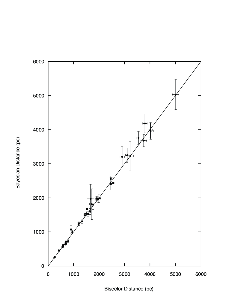
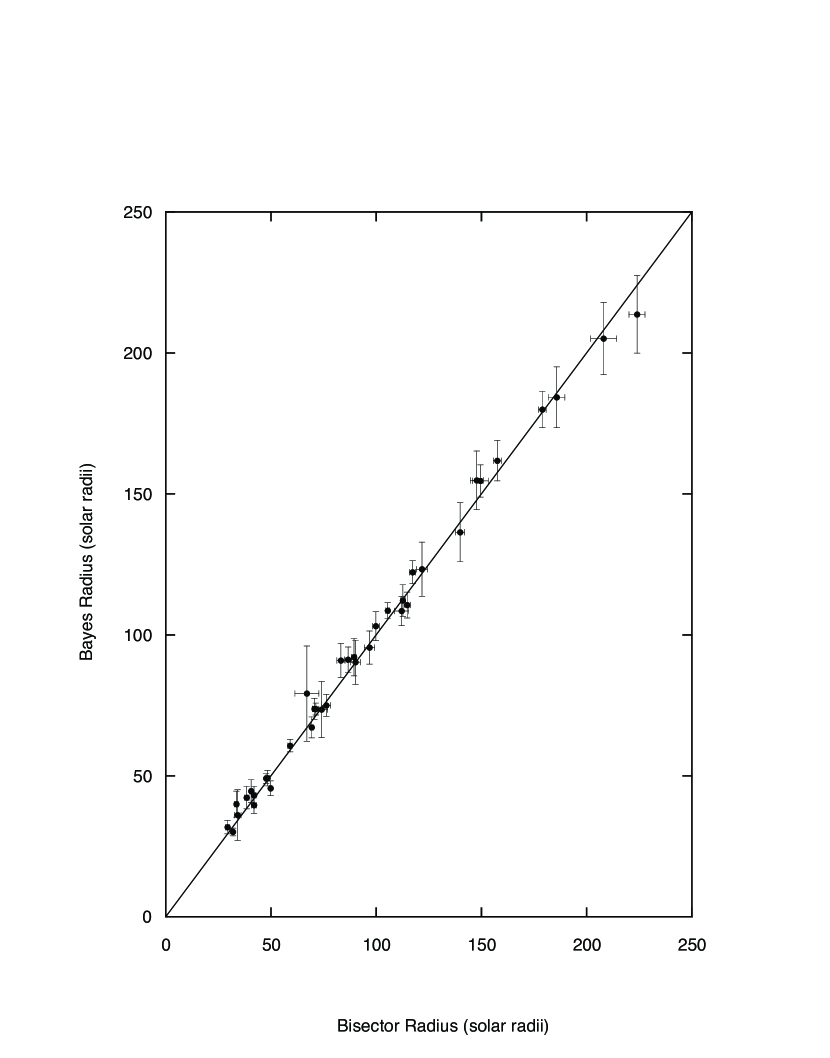
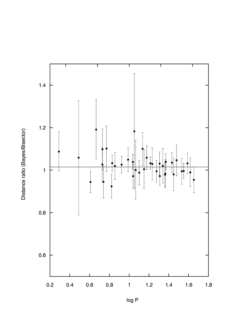
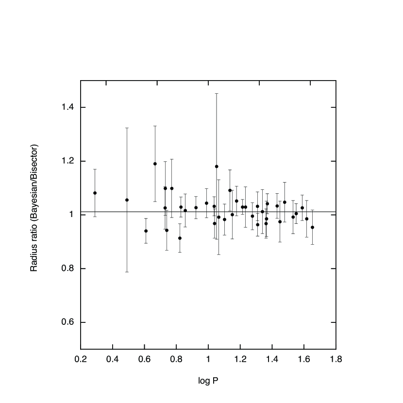
Our goal is to determine differences in the results of the two calculations with respect to distance and radius. Figures 2 and 3 show the Bayesian values plotted against the linear-bisector values. There is no obvious difference between the values from the two calculations. To look for subtle differences, we computed the ratio of the Bayesian distance to the linear-bisector distance. A weighted least-squares fit of this ratio against $log(P)$ gives (Figure 4)

Figure 2: The Bayesian distances are plotted against the linear-bisector distances, each with its 1$\sigma$ error bar. For nearby Cepheids the uncertainties are smaller than the symbols. The identity line is shown for reference.

Figure 3: The Bayesian radii are plotted against the linear-bisector radii, each with its 1$\sigma$ error bar. For smaller Cepheids the uncertainties are comparable to the symbols in size. The identity line is shown for reference.

$$Ratio(r)=1.016(\pm 0.007)-0.012(\pm 0.022)(logP-1.113)$$ (11)

where the fit is centered on the mean period. A weighted fit for the radius ratio gives (Figure 5)

$$Ratio(R)=1.012(\pm 0.007)-0.004(\pm 0.023)(logP-1.113)$$ (12)

These show no evidence for any dependence on pulsation period. Therefore we take a weighted mean for each ratio: the distance calculations differ by $1.5\%\pm 0.6\%$, with the Bayesian being larger, and the radius calculations differ by $1.1\%\pm 0.7\%$, with the Bayesian again being larger. For comparison, the best individual distance and radius measurements in our dataset are for X Cyg, for which the Bayesian uncertainties are both $\pm 2.6\%$, larger than the possible systematic difference between the Bayesian and bisector calculations. Our first result is that the distances and radii computed by the two methods agree quite well.

Figure 4: The ratio of Bayesian distance to bisector distance is plotted against $logP$. The combined uncertainty is shown as a 1$\sigma$ error bar. The line at $ratio=1.016\pm 0.006$ is the weighted mean value.

Figure 5: The ratio of Bayesian radius to bisector radius is plotted against $logP$. The combined uncertainty is shown as a 1$\sigma$ error bar. The line at $ratio=1.012\pm 0.007$ is the weighted mean value.

6.2 Uncertainties in distance and radius

In Figures 4 and 5 the uncertainties can be seen to increase as the period is shorter. This is likely a result of the smaller pulsation amplitudes at shorter periods, which result in the photometric and velocity uncertainties having greater effect on the computed distances and radii.

More importantly, a glance at Table 1, or Figures 4 and 5, shows that the uncertainties in the distances and radii disagree substantially between the two calculations. Typically the Bayesian uncertainty is more than three times the linear-bisector uncertainty.

Figure 6: The posterior probability distribution for the distance to U Sgr is shown as a histogram. A normal distribution of the same mean distance, sigma and area is over-plotted.

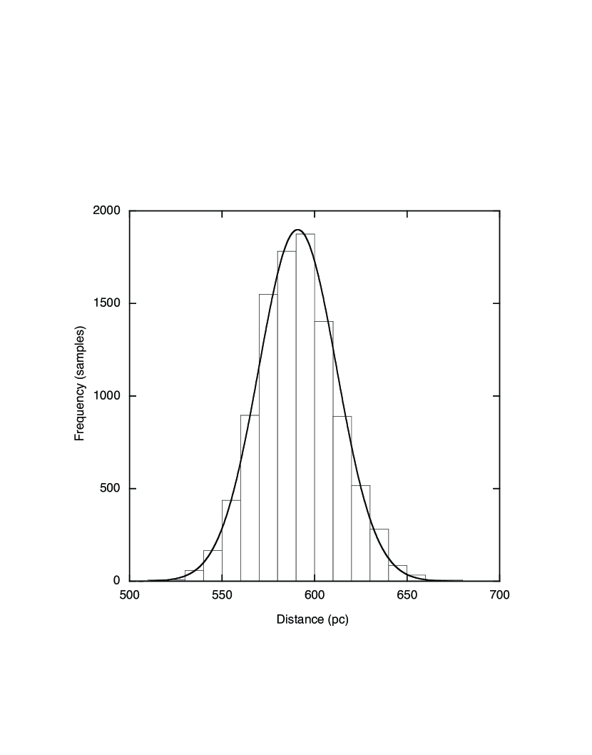
Because the concept of an uncertainty estimated from the Bayesian MCMC posterior probability distribution may not be clear, we show an example in Figure 6, the posterior probability distribution for the distance to U Sgr, which star is typical of our results. Over-plotted on the probability distribution is a normal distribution constructed for the same distance (592 pc), sigma ($\pm 21$ pc) and area (10,000 samples). The normal distribution describes the posterior probability distribution for the distance very well. This justifies our adopting the sigma of the corresponding normal distribution as a 1$\sigma$ estimator for the uncertainty in the distance (and similarly for the radius) determined in the Bayesian calculation. This estimator is then compared to the 1$\sigma$ estimator from the linear-bisector computation.

We add a caveat to the previous paragraph. Because our computation determines the stellar parallax, not the stellar distance, (see equation (10)) the posterior probability distribution for the distance can become asymmetric when the errors are large. As the uncertainties become large, the parallax posterior probability distribution becomes broad (large sigma). Its reciprocal, the distance posterior probability distribution, will also become broad and necessarily asymmetric to larger distances. The same asymmetry will arise for the radius posterior probability distribution in such cases because that distribution is the product of the angular diameter posterior probability distribution (symmetric) and the distance posterior probability distribution (asymmetric). Note that these asymmetric distributions are real and not mathematical artifacts; they properly represent our knowledge of the distance and radius, which is not true for least-squares or maximum-likelihood calculations on the same data. The latter methods assume symmetric errors by their very nature. Because this situation prevails for only a few stars in this sample, and only for stars with large errors, it has little effect on the weighted mean ratios of distances and radii quoted in the previous section.

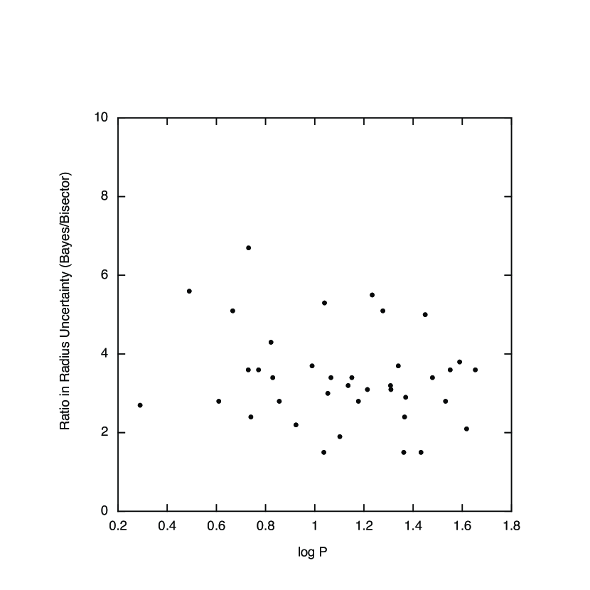
As we did with the distances and radii themselves, we begin by examining the behavior of the ratio of the Bayesian uncertainty to the linear-bisector uncertainty for the same Cepheid. In Figures 7 and 8 we show these ratios for the distance and radius uncertainties plotted against $logP$. Unweighted least-squares fits in these figures yield

$$Ratio(r)=3.396(\pm 0.183)-0.748(\pm 0.549)(logP-1.113)$$ (13)

$$Ratio(R)=3.281(\pm 0.202)-0.673(\pm 0.606)(logP-1.113)$$ (14)

There is no apparent dependence of these ratios on pulsation period. Plots of the ratios of the distance uncertainties against distance and of the ratios of the radius uncertainties against radius are similarly uninformative.

The two ratios are, however, highly correlated with each other ($R=0.99$) as shown in Figure 9. Thus the underlying cause of the larger uncertainties in the Bayesian calculation is likely to be the same for the distance uncertainty and radius uncertainty.

Figure 7: The ratio of the Bayesian distance uncertainty to the bisector distance uncertainty for the same Cepheid is plotted against $logP$.

Figure 8: The ratio of the Bayesian radius uncertainty to the bisector radius uncertainty for the same Cepheid is plotted against $logP$.

Figure 9: The ratio of the Bayesian distance uncertainty to the bisector distance uncertainty is plotted against the ratio of the Bayesian radius uncertainty to the bisector radius uncertainty. The identity line is shown for reference.

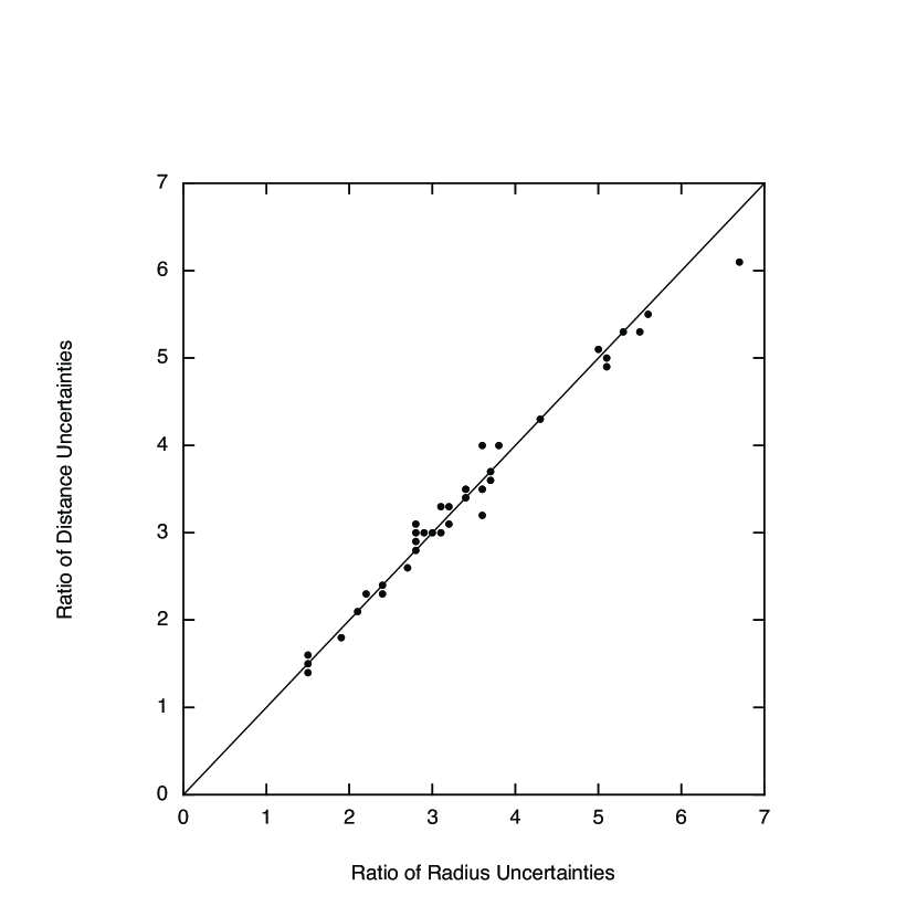
In section 2.1 we noted that the linear-bisector calculation does not treat the errors-in-variables problem rigorously nor does it properly propagate uncertainty through the radial velocity integration. The second of these issues will certainly lead to an underestimate of the uncertainties in the computed distances and radii. Because the Bayesian MCMC calculation does correctly address these two computational issues, we interpret the large ratio of Bayesian to bisector uncertainty as measuring the amount by which the linear-bisector errors have been underestimated. This interpretation is supported by the fact that none of the linear-bisector uncertainties is larger than its Bayesian counterpart. Our second result is that the linear-bisector calculation underestimates the uncertainties in distance and in radius substantially, amounting to factors of 1.4–6.7 for this dataset. This large range implies that the ratio that is obtained depends on the specifics of the data for the Cepheid which varies from star to star.

7 Discussion

We set out to determine whether infrared surface brightness estimates of Cepheid distances and radii by the linear-bisector calculation are affected by the known mathematical shortcomings of that calculation. Based on comparison of Bayesian MCMC and linear-bisector calculations for 38 Cepheids using the same data, same surface brightness equations, and same physical constants, we find that the distances and radii are not adversely affected but that the uncertainties in these quantities are seriously underestimated in the linear-bisector calculation.

We find that Cepheid distances determined by the two calculations agree to $1.5\%\pm 0.6\%$ with the Bayesian distances being larger. This may be compared to the smallest individual uncertainty in distance found in the Bayesian calculation of $\pm 2.6\%$. Similarly we find that Cepheid radii determined by the two calculations agree to $1.1\%\pm 0.7\%$ with the Bayesian radii being larger. This may be compared to the smallest individual uncertainty in radius found in the Bayesian calculation of $\pm 2.6\%$. Any systematic difference between the mathematical approaches is both smaller than a $2\sigma$ effect and smaller than the typical single-star (Bayesian) uncertainty dictated by the data.

These results have an impact on interpretation of infrared surface brightness results for Cepheids. For example, Storm et al. (2005) used six Cepheids in an LMC cluster to infer a distance to the LMC of $(m-M)_{0}=18.30\pm 0.07$ mag. by means of a linear-bisector solution for the infrared surface brightness equations. This is less than the generally accepted distance of 18.50 mag. From the present work, we can say that the linear-bisector calculation used by Storm et al. is not the cause of the smaller distance modulus.

Similarly, that work found a much smaller slope for the Cepheid PL relation in the LMC than had been found by the OGLE project. From the absence of a period dependence between the Bayesian MCMC distances and the linear bisector distances (Fig. 4) and from the overall agreement between the two, we can be certain that the smaller slope found by Storm et al. (2005) is not a result of using the linear-bisector, least-squares method.

The uncertainties in distance and radius determined by the Bayesian MCMC calculation are much larger than determined by the linear-bisector calculation. Given the known problems in a least-squares solution to the surface brightness equations, we interpret this as measuring the amount by which the linear-bisector computation underestimates the uncertainties. It is important to note that the ratio of Bayesian to linear-bisector uncertainty ranges from 1.4 to 6.7 in this set of 38 Cepheids. Clearly the amount by which the linear-bisector method underestimates the uncertainty depends on the specific nature of the data. This is expected, but inconvenient, as it is not possible to simply multiply published linear-bisector uncertainties by a constant correction factor.

Our result on the underestimation of the uncertainties in a linear-bisector calculation is supported in the previously mentioned paper by Storm et al. (2005). As the six Cepheids studied by them are in an LMC cluster, we can be confident that they are at the same distance. The scatter in their distances is then an estimate of the true uncertainty in the linear-bisector distance to the cluster. This scatter was found by Storm et al. (2005) to be twice the formal errors of the linear-bisector distances to the Cepheids, within the range of results determined here.

Other mathematical approaches have been used to solve the surface brightness equations for distance and radius. Ordinary least-squares assumes no error on one variable and all errors on the other. Inverse fit least-squares assumes the reverse. The limitations of ordinary linear least-squares solutions (direct and inverse) include not only underestimation of the errors, but also possible systematic bias in the resulting distances and radii as discussed by Laney & Stobie (1995) and Gieren et al. (1997).

The linear-bisector, least-squares calculation achieves a solution in-between the two other least-squares calculations (direct and inverse). Moreover, the linear-bisector error bar roughly corresponds to the difference between the two least-squares solutions. Maximum likelihood uses information on errors on one or both variables to choose a result between the two results of linear least-squares (direct and inverse fits). As a result, maximum likelihood cannot differ by more than one linear-bisector sigma from ordinary least-squares and even less from a linear-bisector fit. As we have shown that this linear-bisector sigma is about 1/3 of the Bayesian sigma, the maximum likelihood results should also be about 1/3 of the Bayesian values. Our results for the linear-bisector solutions thus suggest that the maximum likelihood method would yield distances and radii in the infrared surface brightness method that are unbiased if the uncertainties in the data are well understood. Unfortunately, these uncertainties are often not well understood. First, Barnes et al. (2003) showed that quoted uncertainties in Cepheid photometry and radial velocities are usually underestimated. Second, maximum-likelihood calculations usually adopt an approximation for the uncertainty in the displacements advocated by Balona (1977) for equally spaced velocity data. Our work demonstrates that this approximation does not apply to typical unequally-spaced radial velocity curves; if it did apply, the linear-bisector method would have yielded uncertainties in distance and radius close to those of the Bayesian MCMC calculation. Thus we expect the maximum likelihood uncertainties to be underestimated as are the linear-bisector uncertainties and for the same reasons.

Table 1: Distance and Radius Results

Cepheid	Period	E(B-V)	$\Delta\theta$	r	$\sigma_{r}$	r	$\sigma_{r}$	R	$\sigma_{R}$	R	$\sigma_{R}$
	days	mag	phase	pc	pc	pc	pc	$R_{\odot}$	$R_{\odot}$	$R_{\odot}$	$R_{\odot}$
				LSQ		Bayes		LSQ		Bayes
SU Cas	1.949322	0.287	0.000	423	$\pm$14	460	$\pm$36	29.4	$\pm$0.9	31.8	$\pm$2.4
EV Sct	3.090990	0.679	0.045	1714	$\pm$83	1815	$\pm$453	34.2	$\pm$1.6	36.1	$\pm$9.0
BF Oph	4.067510	0.247	0.035	705	$\pm$11	666	$\pm$34	32.0	$\pm$0.5	30.1	$\pm$1.4
T Vel	4.639819	0.281	0.000	899	$\pm$25	1071	$\pm$124	33.6	$\pm$0.9	40.0	$\pm$4.6
$\delta$ Cep	5.366341	0.092	0.000	260	$\pm$5	267	$\pm$20	42.0	$\pm$0.9	43.1	$\pm$3.2
CV Mon	5.378793	0.714	0.015	1527	$\pm$24	1677	$\pm$146	40.6	$\pm$0.6	44.6	$\pm$4.0
V Cen	5.49392	0.289	0.000	673	$\pm$20	636	$\pm$48	42.0	$\pm$1.2	39.6	$\pm$2.9
CS Vel	5.904740	0.847	-0.005	2908	$\pm$86	3204	$\pm$297	38.5	$\pm$1.1	42.3	$\pm$4.0
BB Sgr	6.63699	0.284	-0.035	789	$\pm$10	729	$\pm$43	49.9	$\pm$0.6	45.6	$\pm$2.6
U Sgr	6.745226	0.403	0.000	573	$\pm$6	592	$\pm$21	47.7	$\pm$0.5	49.1	$\pm$1.7
$\eta$ Aql	7.176779	0.149	0.000	248	$\pm$5	253	$\pm$15	48.4	$\pm$1.0	49.2	$\pm$2.8
S Sge	8.382086	0.127	-0.010	695	$\pm$11	713	$\pm$25	59.1	$\pm$1.0	60.7	$\pm$2.2
S Nor	9.754244	0.189	0.000	949	$\pm$14	996	$\pm$51	70.7	$\pm$1.0	73.8	$\pm$3.7
Z Lac	10.885642	0.404	-0.005	1905	$\pm$38	1979	$\pm$55	71.4	$\pm$1.4	73.7	$\pm$2.1
XX Cen	10.95337	0.260	-0.040	1647	$\pm$17	1601	$\pm$90	69.4	$\pm$0.7	67.2	$\pm$3.7
V340 Nor	11.287	0.315	0.000	1667	$\pm$142	1972	$\pm$420	67.1	$\pm$5.7	79.2	$\pm$16.9
UU Mus	11.63641	0.413	-0.005	3224	$\pm$125	3227	$\pm$433	74.1	$\pm$2.9	73.5	$\pm$9.9
U Nor	12.643710	0.892	0.000	1325	$\pm$37	1310	$\pm$68	76.3	$\pm$2.1	75.0	$\pm$3.9
BN Pup	13.67310	0.438	0.000	3802	$\pm$88	4184	$\pm$277	83.3	$\pm$1.9	90.9	$\pm$6.0
LS Pup	14.146400	0.478	0.000	5010	$\pm$129	5032	$\pm$438	90.2	$\pm$2.3	90.3	$\pm$7.8
VW Cen	15.03618	0.448	0.000	3550	$\pm$64	3758	$\pm$186	86.7	$\pm$1.6	91.2	$\pm$4.5
X Cyg	16.386332	0.288	0.000	1194	$\pm$10	1233	$\pm$33	105.5	$\pm$0.9	108.6	$\pm$2.8
Y Oph	17.12413	0.655	-0.035	573	$\pm$8	590	$\pm$42	89.5	$\pm$1.2	92.1	$\pm$6.6
VY Car	18.9154892	0.243	-0.020	1968	$\pm$20	1958	$\pm$98	112.7	$\pm$1.1	112.2	$\pm$5.6
RY Sco	20.320144	0.777	0.000	1215	$\pm$19	1253	$\pm$62	99.9	$\pm$1.6	103.1	$\pm$5.1
RZ Vel	20.3969	0.335	0.000	1571	$\pm$21	1527	$\pm$64	114.8	$\pm$1.5	110.6	$\pm$4.6
WZ Sgr	21.8496	0.467	0.000	1764	$\pm$38	1800	$\pm$139	121.8	$\pm$2.6	123.3	$\pm$9.6
WZ Car	23.01320	0.384	0.000	3757	$\pm$114	3678	$\pm$177	112.1	$\pm$3.4	108.5	$\pm$5.2
VZ Pup	23.17100	0.471	0.000	4027	$\pm$104	3962	$\pm$243	96.9	$\pm$2.5	95.5	$\pm$5.9
SW Vel	23.443130	0.349	-0.020	2459	$\pm$28	2557	$\pm$85	117.3	$\pm$1.4	122.2	$\pm$4.1
T Mon	27.03428	0.209	0.000	1439	$\pm$36	1490	$\pm$55	149.6	$\pm$3.8	154.6	$\pm$5.7
RY Vel	28.129259	0.562	-0.005	2458	$\pm$36	2410	$\pm$185	139.9	$\pm$2.1	136.4	$\pm$10.5
AQ Pup	30.1040	0.512	-0.055	3106	$\pm$64	3251	$\pm$216	147.8	$\pm$3.1	154.8	$\pm$10.4
KN Cen	34.029641	0.926	0.005	4011	$\pm$83	3990	$\pm$231	185.8	$\pm$3.9	184.3	$\pm$10.8
$\ell$ Car	35.54804	0.170	-0.025	561	$\pm$6	559	$\pm$19	179.0	$\pm$1.8	179.9	$\pm$6.4
U Car	38.81234	0.283	-0.035	1497	$\pm$17	1545	$\pm$68	157.6	$\pm$1.9	161.8	$\pm$7.2
RS Pup	41.4400	0.446	0.000	2004	$\pm$59	1984	$\pm$122	208.1	$\pm$6.1	205.1	$\pm$12.8
SV Vul	44.994772	0.570	-0.045	2553	$\pm$43	2438	$\pm$149	224.0	$\pm$3.8	213.7	$\pm$13.8

References

- Balona (1977) Balona, L. A. 1977, MNRAS, 178, 231
- Barnes & Evans (1976) Barnes, T. G., & Evans, D. S. 1976, MNRAS, 174, 489
- Barnes & Jefferys (1999) Barnes, T. G., & Jefferys, W. J. 1999, in ASP Conf. Ser. 167, Harmonizing Cosmic Distance Scales in a Post-Hipparcos Era, ed. D. Egret & A. Heck, (San Francisco:ASP), 243
- Barnes et al. (1977) Barnes, T. G., Dominy, J. D., Evans, D. S., Kelton, P. W., Parsons, S. B., & Stover, R. J. 1977, MNRAS, 178, 661
- Barnes, Evans, & Parsons (1996) Barnes, T. G., Evans, D. S., & Parsons, S. B. 1976, MNRAS, 174, 503
- Barnes et al. (2003) Barnes, T. G., Jefferys, W. H., Berger, J. O., Mueller, P. J., Orr, K., & Rodriguez, R. 2003, ApJ, 592, 539; erratum ApJ, 611, 621, 2004
- Fernie (1990) Fernie, J. D. 1990, ApJS, 72, 153
- Fouqué & Gieren (1997) Fouqué, P., & Gieren, W. P. 1997, A&A, 320, 799
- Fouqué et al. (2003) Fouqué, P., Storm, J., & Gieren, W. P. 2003, in Lecture Notes in Physics, Vol. 635, Stellar Candles for the Extragalactic Distance Scale, eds. D. Alloin & W. Gieren (Berlin: Springer), 21
- Gieren, Barnes & Moffett (1989) Gieren, W. P., Barnes, T. G., & Moffett, T. M. 1989, ApJ, 342, 467
- Gieren, Barnes, & Moffett (1993) Gieren, W. P., Barnes, T. G., & Moffett, T. M. 1993, ApJ, 418, 135
- Gieren et al. (1997) Gieren, W. P., Fouqué, P. & Gómez, M. 1997, ApJ, 488, 74
- Gieren et al. (2005) Gieren, W. P., Storm, J., Barnes, T. G., Fouqué, P. Pietrzyński, G., & Kienzle, F. 2005, ApJ, July 10
- Hindsley & Bell (1986) Hindsley, R. B., & Bell, R.A. 1986, PASP, 98, 881
- Isobe et al (1990) Isobe, T., Feigelson, E. D., Akritas, M. G. & Babu, G. J. 1990, ApJ, 364, 104
- Laney & Stobie (1995) Laney, C. D., & Stobie, R. S. 1995, MNRAS, 274, 337
- Nordgren et al. (2002) Nordgren, T. E., Lane, B. F., Hindsley, R. B., & Kervella, P. 2002, AJ, 123, 3380
- Storm et al (2004) Storm, J., Carney, B. W. , Gieren, W. P. , Fouqué, P. , Latham, D. W., & Fry, A.M. 2004, A&A, 415, 531
- Storm et al (2005) Storm, J., Gieren, W. P. , Fouqué, P. , Barnes, T. G., & Gómez, M. 2005, A&A, in press
- Udalski et al. (1999) Udalski, A., Soszyński, I., Szymański, M., Kubiak, M., Pietrzyński, G., Woźniak, P., & Źebruń, K. 1999, Acta Astron., 49, 223
- Welch (1994) Welch, D. L. 1994, AJ, 108, 1421