CMB Tomography: Reconstruction of Adiabatic Primordial Scalar Potential Using Temperature and Polarization Maps

Abstract

Assuming linearity of the perturbations at the time of decoupling, we reconstruct the primordial scalar potential from the temperature and polarization anisotropies in the cosmic microwave background radiation. In doing so we derive an optimal linear filter which, when operated on the spherical harmonic coefficients of the anisotropy maps, returns an estimate of the primordial scalar potential fluctuations in a spherical slice. The reconstruction is best in a thick shell around the decoupling epoch; the quality of the reconstruction depends on the redshift of the slice within this shell. With high quality maps of the temperature and polarization anisotropies it will be possible to obtain a reconstruction of potential fluctuation on scales between $\ell=2$ and $\ell\sim 300$ at the redshift of decoupling, with some information about the three-dimensional shapes of the perturbations in a shell of width 250Mpc.

I Introduction

Cosmic microwave background (CMB) radiation has given us a great deal of insight into the early universe Bennett et al. (2003), for example the pattern of temperature fluctuation gives us the information about the perturbations in the plasma at a temperature $T\sim 3000$K. Using the concordance between big bang nucleosynthesis and CMB Cyburt et al. (2003), we are able to probe directly the earlier universe $T\sim 10^{10}$K, but we rely on an understanding of cosmological theory to learn about the Universe at even higher energy scales. One of the most promising theories of the early universe is inflation Guth (1981), which predicts (i) spatial flatness of the observable universe today, (ii) nearly scale invariant, adiabatic, primordial density perturbations, (iii) homogeneity and isotropy on large angular scales of the observable universe, and (iv) Gaussianity. Predictions (i) and (ii) have been observationally tested Spergel et al. (2003), while predictions (iii) and (iv) are yet to be conclusively tested.

Any characterization of the Gaussianity (or otherwise) of the primordial perturbations will constrain models of inflation (e.g. Starobinsky (1982); Guth and Pi (1982); Bardeen et al. (1983)). Any non-Gaussianity predicted in canonical inflation is very small Acquaviva et al. (2002); Maldacena (2002), but inflation scenarios with large amounts of non-Gaussianity can be constructed Salopek and Bond (1990); Gangui et al. (1994); Gangui (1994). So far, bispectrum tests for primordial non-Gaussianity have not detected a signal in the temperature fluctuations mapped by COBE Komatsu et al. (2002) and WMAP Komatsu et al. (2003a). Other authors have found non-Gaussianity signatures in the WMAP temperature data Mukherjee and Wang (2004); Larson and Wandelt (2004); Vielva et al. (2004); Chiang et al. (2003, 2004). The main motivation of reconstructing primordial potential perturbations is to study these non-Gaussianities. Reconstruction allows us to be more sensitive to the primordial perturbations, which is important because current detections of non-Gaussianity do not specifically select for the primordial perturbations. An advantage of our approach is the ability to use the reconstructed maps to study higher order statistics of the primordial perturbations directly in the reconstructed potential.

We generalize the results from Komatsu et al. (2003b) to use both the temperature and polarization information. We will show that this results in a 3D reconstruction of a thick slice centered at $z_{dec}$. Using the polarization information removes the blind spots which are present at certain scales in the temperature-only analysis. We provide examples that show what will be possible with a future experiment that provide high-fidelity maps of the temperature and E-polarization anisotropies.

We assume that the CMB two-point statistics (i.e. power spectrum) and other sources of cosmological information will reveal the parameters to a high degree of accuracy such that they are input parameters in our reconstruction. If desired our technique can be generalized to include residual uncertainties in cosmological parameters by coupling it to Markov chains.

II Reconstruction of Primordial Fluctuation using Temperature and Polarization

The harmonic coefficients of the CMB anisotropy $(a_{lm})$ are related to primordial fluctuation as:

$$a_{\ell m}^{X}=\frac{2}{\pi}\int k^{2}dk\,r^{2}dr\,[\,\Phi_{\ell m}(r)\,g^{adi}_{X\ell}(k)+S_{\ell m}(r)\,g^{iso}_{X\ell}(k)\,]\,j_{\ell}(kr)$$ (1)

where $\Phi_{\ell m}(r)$ and $S_{\ell m}(r)$ are, respectively, the curvature and the isocurvature harmonic coefficients of the potential at a given comoving distance $r=|\mathbf{r}|$; $g_{X\ell}(r)$ is the radiation transfer function of either adiabatic or isocurvature perturbations; and X refers to either T or E.

Assuming that curvature perturbations $\Phi(\mathbf{\vec{r}})$ dominate over isocurvature perturbations $S(\mathbf{\vec{r}})$, we try to reconstruct the scalar potential $\Phi(r)$ from the observed temperature and polarization of the CMB. A linear filter $O_{\ell}(r)$ which when operated on $a_{\ell m}$ reconstructs the primordial field, can be obtained by minimizing the difference between the filtered field $O_{\ell}(r)a_{\ell m}$ and the underlying field $\Phi_{\ell m}(r)$ Komatsu et al. (2003b). Since the perturbations were in the linear regime when the CMB decoupled, the choice of a linear filter is justified. Positive definiteness of $\frac{\partial^{2}}{\partial{O_{\ell}^{X}(r)}^{2}}$ guarantees a minima of chi square at each $\ell$ and hence guarantees the existence of $O_{\ell}^{X}$.

$$\frac{\partial}{\partial O_{\ell}^{X}(r)}\langle\arrowvert\sum_{X=T,E}\,O_{\ell}^{X}(r)\,a_{\ell m}^{X}-\Phi_{\ell m}(r)\arrowvert^{2}\rangle=0$$ (2)

which gives following form for the filters:

$$\left(\begin{array}[]{c}O_{\ell}^{T}(r)\\ O_{\ell}^{E}(r)\\ \end{array}\right)=\left(\begin{array}[]{ccc}C_{\ell}^{TT}&C_{\ell}^{TE}\\ C_{l}^{TE}&C_{l}^{EE}\\ \end{array}\right)^{-1}\,\left(\begin{array}[]{c}\beta_{\ell}^{T}(r)\\ \beta_{\ell}^{E}(r)\\ \end{array}\right),$$ (3)

where

$$C_{\ell}^{XY}=\langle a_{\ell m}^{X}a_{\ell m}^{*Y}\rangle=\frac{2}{\pi}\int k^{2}dk\,P_{\Phi}(k)\,g_{X\ell}\,g_{Y\ell}(k)$$ (4)

$$\beta_{\ell}^{X}(r)=\langle\Phi_{\ell m}(r)a_{\ell m}^{*X}\rangle=\frac{2}{\pi}\int k^{2}dk\,P_{\Phi}(k)\,g_{X\ell}(k)\,j_{\ell}(kr),$$ (5)

$j_{\ell}(kr)$ being the Bessel function of order $\ell$ and $P_{\Phi}(k)$ is the primordial power spectrum of scalar metric perturbations. In the presence of the instrumental noise, the expression for $C^{XY}_{\ell}$ modifies. Assuming that the noise is Gaussian with variance $\bar{\sigma}^{X}_{\ell m}$, and spatially homogenious; we can write $\bar{\sigma}^{X}_{\ell m}=\bar{\sigma}^{X}_{0}\delta_{\ell\ell^{\prime}}\delta_{mm^{\prime}}$ then $C^{XX}_{\ell}$ is replaced by $C^{XX}_{\ell}+(\bar{\sigma}^{X}_{0})^{2}$. We have assumed that $\bar{\sigma}^{TE}_{lm}$ is zero.

This defines an estimator for the potential

$$\hat{\Phi}_{\ell m}(r)=\sum_{X=T,E}{O_{\ell}^{X}(r)}\,a_{\ell m}^{X}$$ (6)

As evident the equations in (3) are coupled linear equations with variables $O_{\ell}^{T}(r)$ and $O_{\ell}^{E}(r)$.

If only one of the available CMB maps (either temperature T or polarization E) is used to reconstruct the potential, these equations decouple into ordinary linear equations in one variable $O_{\ell}^{X}(r)$ where X can either be T or E. In these special cases Eq. 2 modifies to

$$\frac{\partial}{\partial O_{\ell}^{X}(r)}\langle\arrowvert\,O_{\ell}^{X}(r)\,a_{\ell m}^{X}-\Phi_{\ell m}(r)\arrowvert^{2}\rangle=0$$ (7)

and gives the following form for the filter:

Figure 1: Filters using T and E separately, at five different conformal distances, $r=c(\tau_{o}-\tau_{dec})$, where $\tau_{o}$ is the present conformal time and $\tau_{dec}$ is the conformal time at photon decoupling epoch. We use a $\Lambda$CDM model with re-ionization and $c\tau_{o}=14.2827$Gpc and $c\tau_{dec}=0.2836$Gpc. (a)$O_{\ell}^{T}(r)=\frac{\beta_{\ell}^{T}(r)}{C_{\ell}^{TT}}$ (b)$O_{\ell}^{E}(r)=\frac{\beta_{\ell}^{E}(r)}{C_{\ell}^{EE}}$

$$O_{\ell}^{X}(r)=\frac{\beta_{\ell}^{X}(r)}{C_{\ell}^{XX}}$$ (8)

We have first reconstructed the metric perturbations using the temperature and polarization information separately as given by Eq. 8. Then we solved Eq. 6 to combine the information from temperature T and E polarization and show that reconstruction is much better.

Using both T and E, the expected variance of the reconstructed potential is given by

$$\sigma^{2}_{lm}(r)=\Big{\{}\sum_{X}\frac{(O_{\ell}^{X}(r))^{2}}{\bar{\sigma}^{X}_{\ell m}}+(P^{\phi}_{\ell}(r))^{-1}\Big{\}}^{-1},$$ (9)

where $\bar{\sigma}^{T}_{\ell m}$ and $\bar{\sigma}^{E}_{\ell m}$ are the noise variances in the temperature map and in the polarization map respectively. We define

$$\hat{P}^{\Phi}_{\ell}=\frac{1}{2\ell+1}\sum^{\ell}_{m=-\ell}\hat{\Phi}_{\ell m}\hat{\Phi}^{\ast}_{\ell m}$$ (10)

and use its expectation value:

$$\left<\hat{P}^{\Phi}_{\ell}\right>=(O_{\ell}^{T}(r))^{2}C_{\ell}^{TT}+(O_{\ell}^{E}(r))^{2}C_{\ell}^{EE}+2O_{\ell}^{T}(r)O_{\ell}^{E}(r)C_{\ell}^{TE},$$ (11)

for the purpose of comparing our reconstruction to the theoretical power spectrum. As an estimator of the primordial power spectrum this biased because our filters are optimized for estimating the potential $\Phi_{\ell m}(r)$ and not the power spectrum. This is the standard for optimal, or Wiener, filters, since they remove contamination aggressively. One can compute the bias to correct for this effect and bound the allowed range for the true power spectrum as $\left\langle\hat{P}^{\phi}_{\ell}\right\rangle\pm\sigma^{2}_{\ell}$, where

$$\sigma^{2}_{\ell}(r)=\sqrt{2}\Big{\{}P^{\phi}_{\ell}(r)+(O_{\ell}^{T}(r))^{2}C_{\ell}^{TT}+(O_{\ell}^{E}(r))^{2}C_{\ell}^{EE}$$

$$-2\Big{(}O_{\ell}^{T}(r)\beta_{\ell}^{T}(r)+O_{\ell}^{E}(r)\beta_{\ell}^{E}(r)-O_{\ell}^{T}(r)O_{\ell}^{E}(r)\beta_{\ell}^{TE}(r)\Big{)}\Big{\}}.$$ (12)

Here, $P^{\phi}_{\ell}(r)$ is the theory power spectrum of the potential on a spherical shell of radius $r$.

Figure 2: Reconstructed potential maps in slices centered around the sphere of last scattering $r_{dec}=c(\tau_{o}-\tau_{dec})$. The maps are ordered in decreasing distance, left-to-right and top-to-bottom. The color scale is in dimensionless units of fractional perturbation. Each map is 25 degrees on the side.

III Results

Our examples are computed within a $\Lambda$CDM model with and without re-ionization ($\Omega_{c}=0.26,\Omega_{b}=0.04,\Omega_{\Lambda}=0.7,h=0.7$, scalar spectral index $n_{s}=0.93$, with running $\frac{dn_{s}}{dlnk}=-0.031$, re-ionization optical depth $\tau=0.17$).

Figure 1 shows plots of the operators $O_{\ell}^{X}(r)$ (for X as T and E respectively) for different r as a function of $\ell$. While the reconstruction of the primordial potential will be good on large scales for both T and E (agreeing with the Sachs-Wolfe effect Sachs and Wolfe (1967)) , it will be bad on small scales as $O_{\ell}^{X}(r)$ oscillates about 0 for both T and E. But as a consequence of the physics at decoupling, the transfer functions $g_{T\,\ell}(k)$ and $g_{E\,\ell}(k)$ are out of phase. This results in $O_{\ell}^{T}(r)$ and $O_{\ell}^{E}(r)$ never both being zero at a particular scale (see Figures 3f and 4f). This observation supports our analysis leading to the coupled Eq. 3 and we are able to reconstruct the potential on much broader range of scales if we use both temperature and polarization information from CMB.

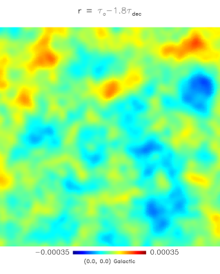
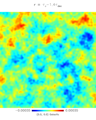
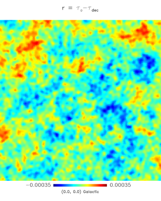
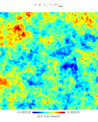
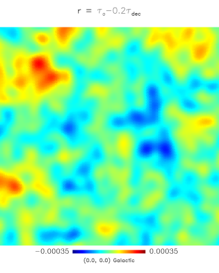
In Figure 2 we show reconstructed potential maps at various slices of conformal time. The quality of reconstruction is sensitive to the reconstruction depth and is best in the thin slice centered on the peak of the differential optical depth. By stacking these slices a three-dimensional thick shell of primordial potential is reconstructed.

Figure 3: Power spectrum of the primordial fluctuation for the $\Lambda$CDM model with re-ionization ($\Omega_{c}=0.26,\Omega_{b}=0.04,\Omega_{\Lambda}=0.7,h=0.7$, $\tau=0.17$, $n_{s}=0.93$, $\frac{dn_{s}}{dlnk}=-0.031$). For all plots the solid line shows the theoretical primordial power spectrum. In (a)-(e) we show the reconstructed power spectrum using the coupled estimator given by Eq. (6) (dashed), bracketed by error bounds (dot-dashed). In (f) we show the reconstructions due to temperature (dashed) and polarization (dot-dashed) alone, using the estimator given by Eq. (8). The theory and the reconstructed power spectrum are shown in arbitrary units.

aaa

Figure 4: Power spectrum of the primordial fluctuation for $\Lambda$CDM model without re-ionization ($\Omega_{c}=0.26,\Omega_{b}=0.04,\Omega_{\Lambda}=0.7,h=0.7$, $\tau=0$,$n_{s}=0.93$, $\frac{dn_{s}}{dlnk}=-0.031$). For all plots the solid line shows the theoretical primordial power spectrum. In (a)-(e) we show the reconstructed power spectrum using the coupled estimator given by Eq. (6) (dashed), bracketed by error bounds (dot-dashed). In (f) we show the reconstructions due to temperature (dashed) and polarization (dot-dashed) alone, using the estimator given by Eq. (8). The theory and the reconstructed power spectrum are shown in arbitrary units.

Figures 3 and 4 show the expected power spectra of the reconstructed potential maps for models with and without re-ionization. The power spectra are bounded from above by the theoretical power spectrum computed from our cosmological parameters $n_{s}$ and $A$. The amount of reconstructed power is indicative of the quality of the reconstruction. As discussed in section II, our filter does not minimize the error bars on this power spectrum. The fact that the error bars include the true spectrum show that the reconstruction of the perturbation itself is unbiased. At small angular scales $\ell\sim 300$ subhorizon physics wash out the information about the primordial fluctuations and the reconstruction fails.

The combination of temperature and E polarization data enables the reconstruction up to $\ell\sim 300$, without blind spots in $\ell$. This is a marked improvement compared to the performance of the operator that uses either temperature or polarization alone which are shown in Figures 3f and 4f.

In Figures 3 and 4 the error bars increase due to cosmic variance on large angular scales. In Figure 3 we see that re-ionization improves the ability to reconstruct the primordial potential at large scales (except in a trough near $\ell\sim 20$). The polarization-only reconstruction reveals that the enlarged E polarization signal due to early re-ionization aids in the reconstruction at very low $\ell$. Physically, the rescattering of photons at low redshift imprints information on the large scale modes of the primordial perturbation Skordis and Silk (2004) .

IV Conclusion and Future Work

We have demonstrated the application of linear theory to construct a least-square estimator of the primordial potential of adiabatic density fluctuations generated during the epoch of inflation. Starting with high-quality maps of the CMB anisotropies in temperature and E polarization and using a fiducial set of cosmological parameters we can reconstruct the primordial potential in a spherical shell of thickness $\sim$ 250Mpc near the peak of the differential optical depth. Reconstruction is reasonably good up to $\ell\sim 300$ and the stronger E polarization signal due to re-ionization aids in reconstructing the potential at very low $\ell$. This effect is consistent with and a generalization of the results by Skordis and Silk Skordis and Silk (2004) who reconstruct the CMB quadrupole with accuracy better than cosmic variance.

To exploit the tomographic techniques we have developed, we require maps of T and E and high signal-to-noise ratios. For this first exploration we have neglected the effect of foregrounds, which will reduce the effective area of the T and E maps that we will be able to use in the reconstruction. One of the advantages of CMB analysis techniques based on Gibbs sampling Jewell et al. (2004); Wandelt et al. (2004) is that methods such as this one can be applied essentially without modification while the messy details of dealing with systematics like foregrounds and instrumental contaminants are taken into account by the Bayesian analysis.

One might wonder whether there are ways to improve on our techniques. In principle this could be done in two distinct ways. First, we might wish to broaden the range in redshift over which we can reconstruct the primordial perturbations. A second way to improve on our techniques would be to enhance the quality of reconstruction.

On the first issue, scattering of cosmic microwave background photons through processes other than Thompson scattering, such as Rayleigh scattering or resonant scattering makes the location of the last scattering surface frequency dependentYu et al. (2001); Hern ndez-Monteagudo and Sunyaev (2005). In principle, this type of effect would allow a more detailed tomography of the inflationary perturbations over a broader range in redshift. However, in the models currently favored by cosmological observations Rayleigh scattering only varies the redshift of the peak in the visibility function by about 1% Yu et al. (2001). This is much less than the thickness of the last scattering surface, and hence does not broaden the redshift range where our reconstruction is effective. A detailed study of the promise of using resonant scattering for this purpose remains to be done.

On the second issue, improving the quality of the reconstruction, it is possible that additional linear combinations of primordial perturbation modes could be constrained by high signal-to-noise CMB maps over a range of frequencies.

Ultimately we envision tests of non-Gaussianity applied to the reconstructed primordial potential. Our filters will select those combinations of the spherical harmonic modes that correlate to the primordial potential. This reduces the probability that residual foregrounds result in a non-Gaussian signature. Further, the ability to reconstruct the potential in a thick shell allows the application of three dimensional shape statistics to potential peaks and troughs. We anticipate the search for non-Gaussianities in the primordial perturbations once high resolution and high sensitivity maps of the E polarization signal become available. To our knowledge the techniques we describe in this paper represent the most direct way to date to probe the statistical properties of the primordial perturbations created in the inflation era.