Likelihood Analysis of GRB Evolution with Redshift

Abstract

We present a likelihood approach to modeling multi-dimensional GRB $E_{pk}$–fluence–redshift data that naturally incorporates instrument detection thresholds. The treatment of instrument thresholds is essential for analyzing evidence for GRB evolution. The method described here compares the data to a uniform jet model, in which the jet parameters are allowed to vary with redshift.

Data from different experiments may be modeled jointly. In addition, BATSE data (for which no redshift information is available) may be incorporated by ascribing to each event a likelihood derived from the full model by integrating the probability density over the unknown redshift. The loss of redshift information is mitigated by the large number of available bursts.

We discuss the implementation of the method, and validation of it using simulated data.

1 Introduction

Analyses of HETE-2- and BeppoSAX-localized Gamma-ray bursts with known redshifts provide evidence that the isotropic-equivalent GRB energy $E_{iso}$evolves with redshift [1]. The assessment of the strength of this evidence is linked with the issue of detection thresholds, which can create apparent energy-redshift correlations by truncation. The modeling of such thresholds is a complex and delicate matter

We present here a method, based on the likelihood function, for analyzing GRB $E_{pk}$–fluence–redshift data in the presence of instrument thresholds. We have developed the method with a view to addressing the question of whether GRB properties do, in fact, evolve with redshift.

2 The Method

We compare observations of GRB data with a model of GRB source properties, using the likelihood function.

The data consists of GRB fluences and $E_{pk}$values, with errors, and GRB afterglow redshifts, where available. We use the results of fits of the Band function to integrated GRB spectra. The fit parameters that we use as data are $y_{pk}\equiv\log_{10}(E_{pk})$ and $y_{A}\equiv\log_{10}(A)$, where $A$ is the amplitude — the scale factor that multiplies the Band function. These parameters are supplemented by their errors, $\sigma_{pk}$and $\sigma_{A}$, respectively.

The model is a generalization of the variable-angle uniform jet model of Lamb, Donaghy and Graziani [2]. The generalization is that the parameters of the distribution of jet opening angles are allowed to evolve with redshift.

The observables of the model are:

• $z$, the redshift.

• $x_{iso}\equiv\log_{10}(E_{iso}/10^{52}~{}\mbox{erg})$.

• $x_{pk}^{(src)}\equiv\log_{10}(E_{pk}^{(src)}/1~{}\mbox{keV})$, where $E_{pk}^{(src)}$is the $E_{pk}$  parameter in the source frame.

• $x_{jet}\equiv\log_{10}(\Omega_{jet}/4\pi)\equiv\log_{10}(1-\cos\theta_{jet})$, where $\theta_{jet}$ is the opening half-angle of the uniform jet.

• $x_{\gamma}\equiv\log_{10}(E_{\gamma}/10^{52}~{}\mbox{erg})$, where $E_{\gamma}$ is the prompt gamma-ray energy actually emitted: $x_{\gamma}=x_{iso}+x_{jet}$.

The model is introduced through the differential event rate:

$$\rho(z,x_{\gamma},x_{jet},x_{pk}^{(src)})dz\,dx_{\gamma}\, dx_{jet} \,dx_{pk}^{(src)}=$$ (1)

$$\mu(z)dz\times\omega(x_{\gamma})dx_{\gamma}\times\kappa(x_{jet}|z)dx_{jet}\times\zeta(x_{pk}^{(src)}|x_{iso})dx_{pk}^{(src)}.$$

where

• $\mu(z)$ is proportional to the Rowan-Robinson [4] SFR function, multiplied by $(1+z)^{-1}dV(z)/dz$, where $V(z)$ is the proper volume of the sphere bounded by redshift $z$.

• $\omega(x_{\gamma})\equiv\exp\left(-\frac{1}{2}\frac{(x_{\gamma}-\bar{x}_{\gamma})^{2}}{\Gamma^{2}}\right)$, with $\Gamma=0.33$ [2] and $\bar{x}_{\gamma}$ a fit parameter.

• $\kappa(x_{jet}|z)\equiv{\Omega_{jet}}^{-\delta}\times\frac{d\Omega_{jet}}{dx_{jet}}$, $\Omega_{jet}^{(1)}<\Omega_{jet}<\Omega_{jet}^{(2)}$. $\delta$, $\Omega_{jet}^{(1)}$, and $\Omega_{jet}^{(2)}$ may be functions of redshift.

• $\zeta(x_{pk}^{(src)}|x_{iso})\equiv\exp\left(-\frac{1}{2}\frac{(x_{pk}^{(src)}-\frac{1}{2}x_{iso}-b)^{2}}{\Lambda^{2}}\right)$, with $b=1.95$ and $\Lambda=0.13$, is the broadened Amati relation [3, 2].

The likelihood function is given by

$$L=\prod_{l=1}^{N_{\mbox{\scriptsize instruments}}}\prod_{i=1}^{N_{l}}\left\{\frac{f(y_{A}^{(l,i)},y_{pk}^{(l,i)},z^{(l,i)})}{\bar{N_{l}}}\right\},$$ (2)

where $\bar{N_{l}}$ is the expected number of events observed by the $l$-th instrument, given its specific threshold, and $f(y_{A}^{(l,i)},y_{pk}^{(l,i)},z^{(l,i)})$ is the individual likelihood of the $i$-th event observed by the $l$-th instrument.

In Eq. (2), the expected number of events $\bar{N}$ is given by

$$\bar{N_{l}}=\int dz\,dx_{jet}\,dx_{\gamma}\,dx_{pk}^{(src)}\,\rho(z,x_{\gamma},x_{jet},x_{pk}^{(src)})\times(\Omega_{jet}/4\pi)\times\eta_{l}(z,x_{iso},x_{pk}^{(src)}).$$ (3)

Note that:

• $\eta_{l}(z,x_{iso},x_{pk}^{(src)})$ is the detection probability by the $l$-th instrument of a GRB whose vital statistics are $z,x_{iso},x_{pk}^{(src)}$. It is here that the instrumental threshold is incorporated. $\eta$ is given by an analytic function that depends on the instrument thresholds. We adopt the threshold values of Band [5].

• The factor $\Omega_{jet}/4\pi$ is the probability that our line-of-sight lies inside the jet.

• $\bar{N_{l}}$ is reducible to a three-dimensional integral over $z$, $x_{iso}$, and $x_{pk}^{(src)}$. This integral must be performed numerically.

In Eq. (2), the event likelihood $f$ is expressed in terms of variables $x_{A}\equiv\log_{10}(A)$, $x_{pk}\equiv\log_{10}(E_{pk})$, which are related to $x_{iso}$, $x_{pk}^{(src)}$by

$$x_{pk}^{(src)} = x_{pk}+\log_{10}(1+z)$$

$$x_{iso} = x_{A}+(\alpha+2)x_{pk}+\log_{10}\left(\frac{d_{L}(z)^{2}}{1+z}\right)-\lambda,$$

where $\alpha$ is the Band-function low-energy power-law index (assumed equal to -1 throughout), $\lambda$ is a unit-conversion constant, and $d_{L}(z)$ is the luminosity distance. We then have

$$f(y_{A},y_{pk},z)= \int dx_{jet}\,dx_{pk}\,dx_{A}\,\rho(z,x_{\gamma}=x_{iso}+x_{jet},x_{jet},x_{pk}^{(src)})$$

$$\times\exp\left[-\frac{1}{2}\frac{(y_{A}-x_{A})^{2}}{\sigma_{A}^{2}}-\frac{1}{2}\frac{(y_{pk}-x_{pk})^{2}}{\sigma_{pk}^{2}}\right].$$

This integral may be performed analytically by standard techniques.

In the case of events for which no redshift is known, the event likelihood should be replaced in the full likelihood by its marginalized version, i.e. $f(y_{A},y_{pk},z)\rightarrow\int_{0}^{\infty}dz\,f(y_{A},y_{pk},z)$.

3 Implementation and Validation

GRB evolution is currently implemented by allowing the three parameters of $\kappa(x_{jet}|z)$ (power-law index, lower- and upper-bounds of power-law domain) to be themselves power-laws in $1+z$. Evolution may be turned off by setting the indices of these power-laws to zero.

The resulting six parameters are supplemented by a seventh — $\bar{x}_{\gamma}$.

The likelihood function is interpreted according to the principles of Bayesian inference. It is converted to a posterior density by multiplication by an assumed prior density on the model parameters. The shape of the resulting probability distribution in parameter space may be used to estimate (or set constraints upon) the parameter values. The peak of the distribution constitutes the best-fit parameter estimate, while confidence regions may be obtained by considering level curves of the posterior density containing prescribed amounts of probability (90%, say).

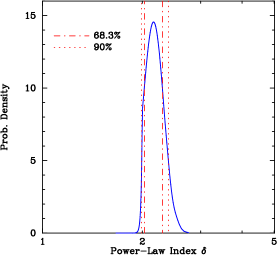
We are currently validating the code by running it on samples of simulated (non-evolving) GRBs produced by the simulator described in [2]. Figure 1 shows the result of estimating the power-law index of the $\Omega_{jet}$ distribution using 25 events drawn from a simulation that assumes an index $\delta=2$. The true value of the index lies within the 90% confidence interval.

Work on estimating $\bar{x}_{\gamma}$ and the other power-law parameters (which are more broadly distributed and more highly correlated) is in progress. We will be applying the experience obtained from analyzing simulations to real data from HETE, BeppoSAX and BATSE in the near future.

Figure 1: Estimating the power-law index of the $\Omega_{jet}$ distribution.

References

• [1] Graziani, C. et al. 2004, in Gamma-Ray Bursts: 30 Years of Discovery, eds. E. E. Fenimore and M. Galassi (New York, AIP), 42
• [2] Lamb, D. Q., Donaghy, T, and Graziani, C. 2005, ApJ, 620, 355
• [3] Amati, L., et al. 2002, A&A, 390, 81
• [4] Rowan-Robinson, M. 2001, ApJ, 549, 745
• [5] Band, D. L. 2003, ApJ, 588, 945