Tightening Constraints from the Lyman Alpha Forest with the Flux Probability Distribution Function

Abstract

The analysis of the Lyman-alpha (Ly$\alpha$) forest of absorption lines in quasar spectra has emerged as a potentially powerful technique to constrain the linear matter power spectrum. In most previous work, the amplitude of the ionizing background was fixed by calibrating simulations to match the observed mean transmitted flux in the Ly$\alpha$ forest. This procedure is undesirable in principle as it requires the estimation of the unabsorbed quasar continuum level, a difficult undertaking subject to various sources of systematic error and bias. We suggest an alternative approach based on measuring the one-point probability distribution function (pdf) of the fluctuations in the flux about the mean, relative to the mean, i.e. the pdf of $\delta_{f}=(f-\langle f\rangle)/\langle f\rangle$. This statistic, while sensitive to the amplitude of the ionizing background, has the virtue that its measurement does not require an estimate of the unabsorbed continuum level. We present a measurement of the pdf of $\delta_{f}$ from seven Keck HIRES spectra, spanning a redshift range of $z=2.2-4.4$. To illustrate that our method is useful, we compare our measurements of the pdf of $\delta_{f}$, and measurements of the flux power spectrum from Croft et al. (2002) at $z=2.72$, with cosmological simulations. From this comparison, we obtain constraints on the mean transmission in the Ly$\alpha$ forest, the slope of the temperature-density relation, as well as the amplitude and slope of the mass power spectrum. Our methodology will be useful for obtaining more precise constraints with larger data samples from the Sloan Digital Sky Survey (SDSS).

1. Introduction

Tremendous progress has been made recently in using the Ly$\alpha$ forest as a cosmological probe. In the emerging theoretical picture of the Ly$\alpha$ forest, most of the structure in the forest is attributed to the gravitational instability. The physics of the absorbing gas is simple; it is just that of gas in photoionization equilibrium with a spatially-homogeneous radiation field. On large scales the hydrogen gas distribution follows the dark matter distribution, and on small scales it is Jeans pressure-smoothed (see e.g., Cen et al. 1994, Zhang et al. 1995, Hernquist et al. 1996, Miralda-Escudé et al. 1996, Muecket et al. 1996, Bi & Davidsen 1997, Bond & Wadsley 1997, Hui et al. 1997, Croft et al. 1998, Theuns et al. 1999, Bryan et al. 1999, Nusser & Haehnelt 1999). In this theoretical picture, each quasar spectrum essentially provides a one-dimensional map of the density field in the intergalactic medium (IGM) at $z\sim 3$, implying constraints on the amplitude and slope of the linear matter power spectrum at $z\sim 3$ and scales of $k\sim 0.1-5h$ Mpc^-1 (see e.g., Croft et al. 1998, McDonald et al. 2000, Croft et al. 2002).

This is a particularly valuable probe since one can infer the linear power spectrum of density fluctuations on scales smaller than those examined by current Cosmic Microwave Background (CMB) experiments and galaxy surveys (Croft et al. 1998). The measurements of the Ly$\alpha$ forest flux power spectrum thus provide an important complement to other probes of large-scale structure, when constraints on small-scale clustering from the Ly$\alpha$ forest are combined with constraints on large scales from CMB experiments. The leverage from the large range of scales probed allows for constraints on neutrino mass (Croft, Hu & Davé 1999, McDonald 2004a, 2004b, Seljak et al. 2004), on warm dark matter (Narayanan et al. 2000, Viel et al. 2005), and on the possibility that the primordial power spectrum deviates from a pure power law (Spergel et al. 2003, Seljak, McDonald, & Makarov 2003, hereafter SMM03, McDonald 2004a, 2004b, Seljak et al. 2004, Viel et al. 2004c).

However, to obtain reliable constraints on the linear matter power spectrum from the Ly$\alpha$ forest, a range of sources of systematic error need to be addressed in more detail. One such source of error is that most previous analyses relied on estimating the unabsorbed quasar continuum level, i.e., the quasar flux in the absence of absorption from the Ly$\alpha$ forest. In particular, measurements of the mean transmitted flux through the Ly$\alpha$ forest were used to calibrate the amplitude of the photo-ionizing background, a crucial input parameter in the theoretical modeling of the Ly$\alpha$ forest. This amplitude can only be constrained from observations in an indirect manner, and it is not feasible to predict this quantity from first principles with anywhere close to the required accuracy. Unfortunately, as SMM03 emphasize, it is difficult to robustly measure the mean transmitted flux in the Ly$\alpha$ forest and hence to constrain the amplitude of the ionizing background with high accuracy.

In order to elaborate further, we briefly describe the measurements of the mean transmitted flux and their difficulties. Two main approaches have been used to estimating the unabsorbed continuum level (see e.g., SMM03). One approach is to extrapolate the continuum from the red side of the Ly$\alpha$ forest, where there is no Ly$\alpha$ absorption. This strategy has been applied by Press, Rybicki, & Schneider (1993), (hereafter PRS93), and by Bernardi et al. (2003). The other method is to locate regions in the Ly$\alpha$ forest where there is apparently no absorption, fit these with a high-order polynomial, and call this the continuum level (Rauch et al. 1997, McDonald et al. 2000).

Each approach has systematic difficulties. The first may cause an underestimate of the mean transmitted flux: This is because, as SMM03 point out, there may be a break in the slope of the quasar continuum near the Ly$\alpha$ emission line; the continuum becoming less steep as one moves across the Ly$\alpha$ line from red to blue, as seen in low redshift quasar spectra (Zheng et al. 1997, Telfer et al. 2002). Furthermore, the slope of the quasar continuum varies significantly from quasar to quasar (Telfer et al. 2002). The fitting together of ‘unabsorbed’ regions in the second method adds an undesirable subjective element to the data analysis, and inevitably breaks down at sufficiently high redshift where there are no, or very few, unabsorbed regions in the Ly$\alpha$ forest. This approach tends to overestimate the mean transmitted flux in the Ly$\alpha$ forest. There is yet another difficulty with this type of continuum fitting. The difficulty arises because quasar spectra are typically taken with an echellograph. The full quasar spectrum is then pieced together from several individual echelle orders, with the signal to noise of the spectrum dropping off near the edges of each echelle order (see e.g. Hui et al. 2001). This imprints a periodic structure in the noise, an added obstacle in continuum estimation.

In contrast to the measurements of the mean transmitted flux, the unabsorbed quasar continuum level does not need to be estimated in order to measure the flux power spectrum. In measuring the flux power spectrum, the power spectrum of the fluctuations in the flux about the mean, relative to the mean is the quantity of interest. That is, the power spectrum of $\delta_{f}=(f-\langle f\rangle)/\langle f\rangle$ is estimated. To determine this quantity observationally, the mean flux $\langle f\rangle$ (Hui et al. 2001, Croft et al. 2002) can be measured directly, without first rescaling to the unabsorbed continuum level. This statistic is sensitive to the shape of the continuum, since the continuum, and hence the mean flux, varies slowly across a quasar spectrum, but it is not sensitive to the normalization of the quasar continuum. It is thereby preferable to have a method of calibrating the amplitude of the ionizing background that does not depend on estimating the normalization of the quasar continuum.

Furthermore, when measurements of the flux power spectrum are combined with measurements of the mean transmitted flux, the resulting constraints on the linear matter power spectrum depend sensitively on the assumed mean transmitted flux (Croft et al. 2002, Zaldarriaga et al. 2001a, Zaldarriaga et al. 2003, SMM03). This is because the effect of changing the amplitude of the ionizing background on the flux power spectrum is rather degenerate with the effect of varying the linear matter power spectrum.

Additional information, beyond that contained in the flux power spectrum, is therefore necessary to simultaneously constrain the linear matter power spectrum and the amplitude of the ionizing background. McDonald et al. (2004b), however, note that variations in the linear power spectrum and the mean transmission, affect the flux power spectrum differently at different redshifts. Therefore they can break the degeneracy that we mention using only measurements of the flux power spectrum, by virtue of the long redshift span and high statistical precision of data from the SDSS. For this to work, they must assume that the mean transmission and other nuisance parameters evolve smoothly with redshift. The technique we will describe below can provide a useful check of these assumptions, and possibly tighten their constraints further. For this purpose, an alternative to the usual source of ‘additional information’, the mean transmitted flux, is desirable.

Croft et al. (2002) suggest one such alternative method for calibrating the amplitude of the ionizing background based on measuring the number of times the flux crosses a given threshold in an observed quasar spectrum and comparing this with the threshold crossing frequency in simulated quasar spectra. In this paper, we take this suggestion a step further by measuring the full probability distribution function (pdf) of $\delta_{f}$, which also does not require an estimate of the unabsorbed continuum level. We find that this quantity itself is sensitive to the amplitude of the ionizing background, and we thereby sidestep one of the biggest loopholes in parameter estimation from the Ly$\alpha$ forest – by going straight from quasar spectra to parameter constraints without continuum fitting.

This extends previous work which measured the probability distribution of flux (normalized to the unabsorbed continuum level) and compared to simulations. In particular, Rauch et al. (1997) and McDonald et al. (2000), found that canonical $\Lambda$CDM models provide a good match to the observed probability distribution of the flux (normalized to the unabsorbed continuum level), and Gaztanaga & Croft (1999) studied the one-point flux pdf in the context of the gravitational instability model of the Ly$\alpha$ forest. Desjacques and Nusser (2004) also recently emphasized the advantage of using the pdf of the flux (normalized to the unabsorbed continuum level) along with the flux power spectrum to constrain the linear matter power spectrum.

In the present paper, we first measure the pdf of $\delta_{f}$, and demonstrate that this quantity is insensitive to the behavior of the quasar continuum. Next, we combine our measurement of the pdf of $\delta_{f}$ with the flux power spectrum measurements of Croft et al. (2002) at $z=2.72$. Our intention here is simply to illustrate that the pdf of $\delta_{f}$ is useful, when employed in conjunction with the usual flux power spectrum, for constraining cosmological parameters and the parameters that describe the physics of the IGM. Our measurements of the pdf of $\delta_{f}$ can be combined with more precise measurements of the flux power spectrum from SDSS data (from McDonald 2004a, or Hui et al. in prep.). In addition, the pdf of $\delta_{f}$ can itself be well-measured from SDSS data (Burgess, Burles et al. in prep.). Measurements of the pdf of $\delta_{f}$ may be regarded as part of a larger effort to incorporate higher order statistics into the analysis of the Ly$\alpha$ forest, as suggested by Zaldarriaga et al. (2001b), Mandelbaum et al. (2003), and Viel et al. (2004a). The pdf, as a one point statistic, is a sensible starting place for incorporating higher-order statistics into the analysis of the Ly$\alpha$ forest.

The outline of the paper is as follows. In §2 we illustrate the degeneracy between the amplitude and slope of the mass power spectrum and the mean transmitted flux in the Ly$\alpha$ forest, reiterating the main points of SMM03. In §3 we present a measurement of the pdf of $\delta_{f}$ from Keck HIRES data and show that our measurement is robust to the treatment of the quasar continuum. In §4 we illustrate how the measurement of the pdf of $\delta_{f}$ helps to tighten constraints on the slope and amplitude of the mass power spectrum. In §5 we present constraints on the slope of the temperature-density relation, and in §6 we conclude. In the Appendix, we present some details regarding our simulations, and examine the convergence of our results with respect to simulation resolution and box size. Tables of the measurements presented in this paper are available electronically at the website http://t8web.lanl.gov/people/heitmann/lyma/.

2. Degeneracy between the amplitude and slope of the matter power spectrum and the mean transmitted flux

In this section we illustrate the degeneracy between the amplitude of the mass power spectrum and the mean flux in the Ly$\alpha$ forest. We first demonstrate that in the absence of assumptions about the mean flux in the Ly$\alpha$ forest, only very weak constraints on the amplitude and slope of the linear mass power spectrum are obtained (SMM03). We illustrate our points using observational measurements of the flux power spectrum from Croft et al. (2002) at a redshift of $\langle z\rangle=2.72$. In order to introduce notation, we provide a very brief recap of theoretical models of the Ly$\alpha$ forest. For more details the reader is referred to e.g, Hui et al. (1997).

Assuming photo-ionization equilibrium, the optical depth to Ly$\alpha$ absorption is given by

$$\tau=A(1+\delta)^{2-0.7\alpha}.$$ (1)

Here $\delta$ is the gas over-density and $\alpha$ is the power law in the temperature-density relation, i.e., $T=T_{0}(1+\delta)^{\alpha}$. The parameter A is proportional to (e.g., Rauch et al. 1997, Hui et al. 2001)

$$A\propto\left(\Omega_{b}h^{2}\right)^{2}\frac{T_{0}^{-0.7}}{\Gamma_{\rm HI}}\frac{H_{0}}{H(z)}\left(1+z\right)^{6},$$ (2)

where $\Omega_{b}$ is the baryon density in units of the critical density, $H(z)$ is the Hubble parameter at redshift $z$, $H_{0}$ is the Hubble parameter today, $h$ is $H_{0}/100$ km/s/Mpc, and $\Gamma_{\rm HI}$ is the photoionization rate of hydrogen, which is directly proportional to the amplitude of the ionizing background. The parameter $A$ is determined by a product of cosmological parameters, which are known to high accuracy, with the combination $T_{0}^{-0.7}/\Gamma_{\rm HI}$, which is uncertain. The optical depth is then shifted into redshift space and convolved with a thermal broadening window. The flux transmitted through the Ly$\alpha$ forest is given by $F/F_{c}=e^{-\tau}$, and the amount of flux absorbed by the Ly$\alpha$ forest is $1-F/F_{c}$. Here $F/F_{c}$ denotes the flux normalized to the unabsorbed quasar continuum level. Our model of the Ly$\alpha$ forest is then complete given the baryonic matter density and peculiar velocity fields specified by our numerical simulations for a given cosmological model (see the Appendix for details regarding simulations).

Our methodology for obtaining constraints on the matter power spectrum and the physics of the IGM from this modeling is very similar to that of Zaldarriaga et al. (2001a, 2003) (see also Lidz et al. 2003). In brief, we generate the flux power spectrum and pdf for a large grid of simulated models, calculate the likelihood of the model given the data, and marginalize over nuisance parameters to obtain constraints on the amplitude and slope of the linear matter power spectrum. For this purpose, we ran a grid of models describing the IGM, with parameter vector $(a,n,T_{0},\alpha,\langle F/F_{c}\rangle)$. Our grid covers the following range in each parameter:

• $a=(0.0919,0.1301,0.1479,0.1682,0.1914,0.2178,\\ 0.2480,0.2827,0.3227,0.3691,0.4236,0.5327)$

• $n=(0.7,0.8,0.9,1.0,1.1,1.2,1.3)$

• $T_{0}=(200,250,300,350,400,\\ 450)$ (km/s)²

• $\alpha=(0.0,0.1,0.2,0.3,0.4,0.5,0.6)$

• $\langle F/F_{c}\rangle=(0.670,0.680,0.685,0.690,0.695,0.700,\\ 0.705,0.710,0.715,0.720,0.725,0.730,0.735,0.740,\\ 0.745,0.750,0.755,0.760,0.770,0.780)$

The parameters of our simulated model are : $a$, the scale factor of the simulation output, which effectively corresponds to the normalization of the matter power spectrum; $n$, the slope of the primordial power spectrum, each slope corresponding to a different linear power spectrum slope on the scales probed by the Ly$\alpha$ forest; $T_{0}$, the temperature at mean density; $\alpha$, the slope of the temperature density relation and $\langle F/F_{c}\rangle$, the mean transmission in the Ly$\alpha$ forest. In this paper we generally parameterize our model in terms of the mean transmission, $\langle F/F_{c}\rangle$, although varying this parameter corresponds to varying $A$ and hence the amplitude of the ionizing background [Eqn. (2)]. We emphasize that, in later parts of the paper, we do not use measurements of the mean transmission to fix the amplitude of the ionizing background. In spite of this we will still parameterize our model in terms of $\langle F/F_{c}\rangle$, rather than in terms of the amplitude of the ionizing background. This will be convenient for comparing our results with different measurements of $\langle F/F_{c}\rangle$ that appear in the literature. In addition to these parameters, we need to specify a thermal history in order to calculate the gas pressure term in our HPM simulations. We describe this in the Appendix.

In this paper we use large volume simulations, which lack sufficient resolution to completely resolve the small-scale structure in the Ly$\alpha$ forest. Hence, in comparing our simulated models of the flux power spectrum with Croft et al. (2002)’s measurements, we confine the comparison to scales of $k\lesssim 0.02$ s/km. In the Appendix, we demonstrate that even restricting our analysis to these scales our simulation resolution is somewhat marginal, and we attempt to quantify the resulting systematic error. We will generally quote constraints on the amplitude and slope of the matter power spectrum as constraints on the dimensionless amplitude of the power spectrum at redshift $z$ and scale $k_{p}=0.03$ s/km, $\Delta^{2}=k_{p}^{3}P(k_{p},z)/2\pi^{2}$, and the logarithmic slope at the same scale and redshift, $n_{\rm eff}=d{\rm ln}P(k_{p})/d{\rm ln}k$ (Croft et al. 2002). For reference, at $z=2.72$, the central redshift of the data sample in Croft et al. (2002), the scale $k_{p}$ corresponds to a co-moving scale of $k_{0}=H(z=2.72)/(1+z)k_{p}$, which is $k_{0}=3.24h$ Mpc^-1 for a flat, $\Lambda$CDM cosmology with matter density $\Omega_{m}=0.3$.

Next, we have to consider the priors we should adopt on the different nuisance parameters involved in the modeling. For the most part, we will be fairly conservative in adopting these priors. The temperature of the IGM, however, has been constrained using simulations with smaller volume, but higher resolution than our present simulations (see, e.g., McDonald et al. 2001, Zaldarriaga et al. 2001a). The most pronounced effect of gas temperature on the flux power spectrum is a small-scale smoothing on scales of $k\gtrsim 0.05$ s/km. Since these scales are not fully resolved by our simulations, we will not attempt to constrain $T_{0}$ with the present simulations. Motivated by results from the higher resolution simulations, however, we adopt a prior on the temperature of the IGM of $T_{0}=300\pm 50$ (km/s)². (We will relax our prior on $T_{0}$ in §5 to demonstrate that our constraint on the temperature-density relation, $\alpha$, is not sensitive to the prior on $T_{0}$.) This prior on the temperature corresponds to the constraint found by McDonald et al. (2001), except with an error bar approximately twice as large. Conservatively, we will let $\alpha$ vary freely over the entire physically allowed range of $\alpha=0.0-0.6$ (Hui & Gnedin 1997). There is one sense in which we are not conservative, however: in calculating the gas pressure term in our HPM simulations, we fix the thermal history of the IGM (see the Appendix for details). This was done partly to reduce computational burden, but also because, on the large scales we consider here ($k\lesssim 0.02$ s/km), the effects of gas pressure smoothing are likely to be sub-dominant compared to the size of Croft et al. (2002)’s error bars.

With this in mind, we generate the flux auto spectrum for each model in our grid and compute the likelihood of the model given the data. We show the resulting likelihood contours in §4. Presently, we illustrate the degeneracy between $\langle F/F_{c}\rangle$ and the amplitude and slope of the mass power spectrum, with example model fits from our grid. The model fits each have very different mass power spectrum amplitudes and slopes, compensated by rather different values of the mean flux, and somewhat by small changes in the other nuisance parameters. This is shown in Figure 1. In this plot, one can see that, assuming nothing about the mean flux in the Ly$\alpha$ forest, the amplitude of the mass power spectrum is uncertain by an order of magnitude, and the slope of the mass power spectrum has an error of at least $20\%$. While the range of values for the mean transmitted flux considered in the figure is perhaps excessively conservative, a wide range of mean transmitted flux priors have been considered in the literature. Specifically, the prior on the mean transmission adopted by Croft et al. (2002), is $\langle F/F_{c}\rangle=0.705\pm 0.012$, while SMM03 consider two priors based on the measurements of McDonald et al. (2000): $\langle F/F_{c}\rangle=0.742\pm 0.012$, and one with expanded error bars, $\langle F/F_{c}\rangle=0.742\pm 0.027$, and Viel et al. (2004b) adopt $\langle F/F_{c}\rangle=0.730\pm 0.011$. The best fit amplitude of the mass power spectrum with the Croft et al. (2002) prior on the mean transmitted flux differs by a factor of $\gtrsim 2$ than that obtained with the SMM03 prior (see the models in Figure 1). Furthermore, SMM03 show that the error contours become very large with their prior on the mean transmitted flux, in comparison with the error contours corresponding to the Croft et al. (2002) prior. The flux field becomes primarily sensitive to larger and larger over-densities as the mean transmitted flux increases, and one loses sensitivity to the linear matter power spectrum (see also Zaldarriaga et al. 2003). The figure also illustrates that including information at high $k$, (we only compare theory with data on scales of $k\lesssim 0.02$ s/km due to the limited resolution of our simulations), would only help slightly in obtaining tighter constraints.

Figure 1.— Auto spectrum from Croft et al. (2002) at $\langle z\rangle=2.72$ compared to models that compensate for their very different mass power spectrum amplitudes and slopes by having different mean transmissions. In our subsequent analysis, we only compare theoretical models with data on scales of $k$ less than $0.02$ s/km owing to our limited simulation resolution. The models are completely specified by the parameter vector $(\Delta^{2},n_{\rm eff},T_{0},\alpha,\langle F/F_{c}\rangle)$. The models shown are specified by the following parameter sets: $(0.37,-2.68,350,0.5,0.680)$, $(0.71,-2.58,300,0.4,0.720)$, $(1.04,-2.48,300,0.4,0.735)$, $(1.53,-2.38,300,0.4,0.750)$, $(3.29,-2.18,300,0.3,0.770)$.

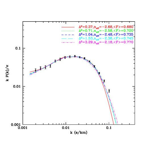
The lesson here, reiterating the main point of SMM03, as well as cautions mentioned by Croft et al. (2002), is that one needs a tight constraint on the mean transmission in the Ly$\alpha$ forest in order to derive constraints on the mass power spectrum from the Ly$\alpha$ forest flux power spectrum. There are a few possible ways to circumvent this difficulty. One approach is to determine any bias in estimates of the mean absorption obtained by fitting together ‘unabsorbed’ regions in the Ly$\alpha$ forest using simulated spectra, as Rauch et al. (1997) and McDonald et al. (2000) attempted to do. An inherent difficulty is that mock spectra are typically produced in simulation boxes that are small compared to the length of spectra over which the continuum-fitting procedure is performed. Furthermore, the size of the estimated bias may be model-dependent. Another approach might be to correct estimates of the unabsorbed quasar continuum level extracted from the red side of Ly$\alpha$ based on the break found in low redshift quasar spectra. However, the correction depends on the position of the break, which is poorly determined from the low redshift quasar spectra. As we mentioned in the Introduction, McDonald et al. (2004b) circumvent the degeneracy we mention by exploiting the fact that the flux power spectrum depends differently on the modeling parameters at different redshifts. The disadvantage of this approach is that they must assume that the nuisance parameters evolve smoothly with redshift. Yet a different approach, which we pursue presently, is to avoid using the mean transmitted flux at all, and to instead calibrate the amplitude of the ionizing background, [or equivalently the parameter $A$ in Eqn. (2)], using a different statistic entirely.

3. Measuring the probability distribution of the flux field and its error bars

In this section, we present a measurement of the probability distribution of the flux field, $\delta_{f}$, which will be useful in calibrating the parameter $A$ in Eqn. (2), as we will demonstrate. We choose a particular estimator for $\delta_{f}$ that we can measure robustly from the data sample as well as the numerical simulations. Our objectives here are to: 1) Choose a quantity that can be measured accurately from our simulations, 2) Use an estimator of $\delta_{f}$ that does not rely on estimating the level of the unabsorbed quasar continuum, 3) Identify an estimator that is insensitive to contamination from the unknown shape of the quasar continuum.

Several different estimators for $\delta_{f}$ have been discussed in the literature in the context of measuring the flux power spectrum (Hui et al. 2001, Croft et al. 2002). We now briefly describe these estimators. The number of photon counts, $N_{p}$, in the Ly$\alpha$ forest portion of a quasar spectrum is the product of a slowly varying quasar continuum, $N_{c}$, with $e^{-\tau}$, (ignoring additional opacity from metal absorption lines). Fluctuations in $N_{p}$ arising from fluctuations in $e^{-\tau}$ have to be separated out from those that arise due to structure in the quasar continuum. This can be accomplished, at least on sufficiently small scales, since the quasar continuum, $N_{c}$, varies smoothly in comparison to $e^{-\tau}$. We proceed to discuss how this is done. The mean transmission, i.e., $e^{-\tau}$ averaged over an ensemble of quasar spectra, $\langle F/F_{c}\rangle=\langle e^{-\tau}\rangle$, is not a function of wavelength for a sufficiently small stretch of a quasar spectrum. In spite of this, the mean number of photon counts depends on wavelength due to the slowly varying structure in the quasar continuum. This ‘running mean’ quasar count can be estimated from the spectrum by fitting a low order polynomial to the quasar spectrum (Hui et al. 2001), or by smoothing the spectrum with a large radius filter (Croft et al. 2002). Then $\delta_{f}$ is formed by subtracting the running mean quasar count from the raw quasar count, finally dividing out by the running mean. This procedure thereby offers a means of forming $\delta_{f}$ and measuring its flux power spectrum without first estimating the normalization of the quasar continuum.

The estimator we use for $\delta_{f}$ in measuring the flux pdf is very similar to the estimator used by Croft et al. (2002) for measuring the flux power spectrum. In particular, we will demonstrate that $\delta_{f}$ defined by:

$$\delta_{f}(\lambda)=\frac{f_{r}(\lambda)-f_{R}(\lambda)}{f_{R}(\lambda)}$$ (3)

satisfies the three desired criteria we outline above. In this equation $f_{r}(\lambda)$ indicates the value of the flux field, $f$, at wavelength $\lambda$ when smoothed with a Gaussian filter of radius $r$ – i.e., the variance of the Gaussian is $\sigma^{2}=r^{2}$, and $f_{R}(\lambda)$ denotes the flux field at wavelength $\lambda$ when smoothed with a Gaussian filter of radius $R$. The filter, $r$, has a small radius, and serves to take out small-scale power on scales that are under-resolved in our simulation. In the Appendix we demonstrate that $r=30$ km/s is an appropriate filter for our present simulations. The filter, $R$, represents a large-scale smoothing that defines the running-mean flux in the quasar spectrum. Given a sample of quasar spectra it is straightforward to estimate $\delta_{f}$ as defined above, and measure its one-point probability distribution function.

We carry out this procedure using spectra obtained with the High Resolution Echelle Spectograph (HIRES) on the Keck telescope. These quasar spectra are the same as described in Rauch et al. (1997) and in McDonald et al. (2000). (See these papers for references regarding the data reduction procedure.) The resolution of the quasar spectra is FWHM $\sim 6.6$ km/s and the typical signal to noise per $0.04\AA$ pixel is $S/N\sim 50$. The quasar spectra, listed by name, emission redshift, and wavelength range examined, are shown in Table 2. Before measuring the flux pdf, but after performing the smoothing procedure described by Eqn. (3), we attempt to cut out metal lines, damped-lyman alpha systems, and spurious pixels, using wavelength cuts similar to those in Rauch et al. (1997) and McDonald et al. (2000). Unlike Rauch et al. (1997) and McDonald et al. (2000), we use only the ‘raw’ data, as opposed to continuum-fitted data, in making our measurements.

We split the data sample into four relatively narrow redshift bins, and measure the flux pdf in each redshift bin. The redshift bins are defined in Table 1 below. One of the redshift bins is chosen to have a mean redshift of $z=2.72$, the central redshift of the Croft et al. (2002) sample. In the present paper, we will limit our theoretical analysis to this redshift bin, and we will use it to illustrate our procedure for measuring the flux pdf.

Table 1Redshift Bins for PDF measurements

$z_{\rm low}$	$z_{\rm high}$	$\langle z\rangle$
2.20	2.45	2.26
2.46	3.00	2.72
3.01	3.70	3.28
3.71	4.43	3.99

After splitting our data sample into several redshift bins, we smooth each quasar spectrum in order to form $\delta_{f}$ as described above, and then re-bin each spectrum into pixels of size $20$ km/s. Data within $2,000$ km/s, (which corresponds to $4$ times the radius of our large-scale smoothing filter, $R$), of the edge of each spectrum are cut after performing the smoothing to avoid edge effects. Upon forming the flux field from each quasar spectrum, we measure the pdf using $36$ bins in $\delta_{f}$, each with a width of $0.061538$. The center of the lowest flux bin corresponds to $\delta_{f}=-1.01538$. In the event that a pixel has flux lower (higher) than the lower (upper) edge of the smallest (largest) $\delta_{f}$ bin it is included in the lowest (highest) $\delta_{f}$ bin. We compute the average flux in each bin, and use this, rather than the bin center, when comparing with theoretical models. as allows

Next, we discuss our procedure for estimating error bars. In order to measure the variance and covariance of our estimates of the pdf of $\delta_{f}$, we use a jackknife technique. Specifically, we 1) estimate the pdf from the full data sample, 2) divide the data set into $n_{g}=30$ different subgroups, and 3) we estimate the pdf of the data sample omitting each sub-group. Let $\hat{P}(\delta_{i})$ represent the pdf estimated from the full data sample for a bin with average flux, $\delta_{i}$. In addition, let $\tilde{P}_{k}(\delta_{i})$ represent the same quantity, estimated not from the full data sample, but from a data sample that omits the pixels in the kth subgroup. Then the jackknife estimate of the covariance between the estimates of the pdf in a bin with average flux, $\delta_{i}$, and a bin with average flux, $\delta_{j}$ is given by:

$$Cov(i,j)=\sum_{k=1}^{n_{g}}\left[\hat{P}(\delta_{i})-\tilde{P}_{k}(\delta_{i})\right]\left[\hat{P}(\delta_{j})-\tilde{P}_{k}(\delta_{j})\right]$$ (4)

and the diagonal variance, for a bin with flux $\delta_{i}$, is $\sigma^{2}_{i}=Cov(i,i)$.

Figure 2.— A demonstration that our lognormal model roughly reproduces the pdf of the data.

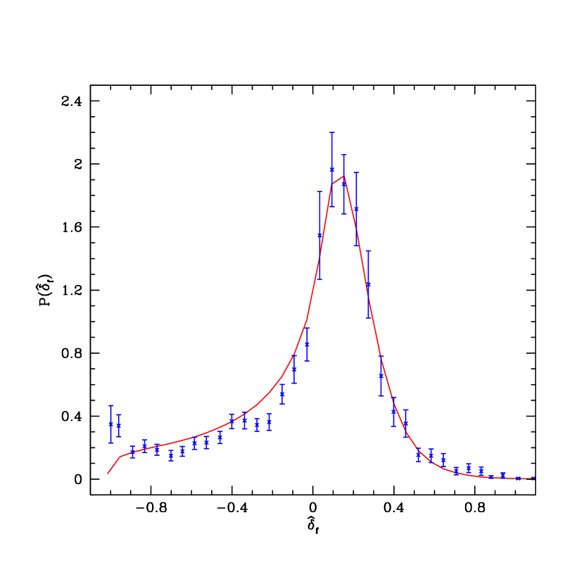
In order to check the accuracy of our jackknife estimate of the error bars, we generate mock spectra using the lognormal model described in McDonald et al. (2004a). This provides a test of our error estimation procedure: first we measure the dispersion across many independent realizations generated using our lognormal simulations, and second we make a jackknife estimate from a single realization. To the extent that the jackknife method agrees with error bars estimated from many independent realizations, we can be confident that it is sound. We illustrate our procedure for constructing mock realizations of the data considering the redshift bin centered on $\langle z\rangle=2.72$ as an example. The corresponding procedure for the other redshift bins is very similar. First we generate four lines of sight, corresponding to the number of lines of sight in our actual data sample that fall into the $\langle z\rangle=2.72$ bin. Each line of sight spans the length of our redshift bin, $z=2.46-3.00$, on a fine grid of $16384$ pixels. We form $\delta_{f}$ according to Eqn. (3), coarse-sample onto pixels of size $20$ km/s, and cut out regions of spectra until the mock spectra have exactly the same wavelength coverage as the actual spectra. In Figure 2, we show a measurement of the pdf from many realizations of our lognormal model as compared to a measurement of the pdf from real data. The comparison illustrates that the lognormal model roughly reproduces the pdf of the actual data, although there are some differences between the model and data. We emphasize that we only use the lognormal model to 1) test our jackknife estimates of the variance of the pdf, 2) indicate the correlation coefficient between our estimates of the pdf in different flux bins. This second step is necessary because, as we detail below, our estimates of the off-diagonal elements of the covariance matrix from our present data set are too noisy to be useful. In the future, with larger data samples, we can just estimate the covariance matrix directly.

Figure 3.— Comparison of two estimates of the error bars on the flux pdf, as measured from lognormal simulations. The first error bar estimate comes from the dispersion across many independent realizations, and the second is a jackknife estimate. The fractional difference between the fractional error bars is shown.

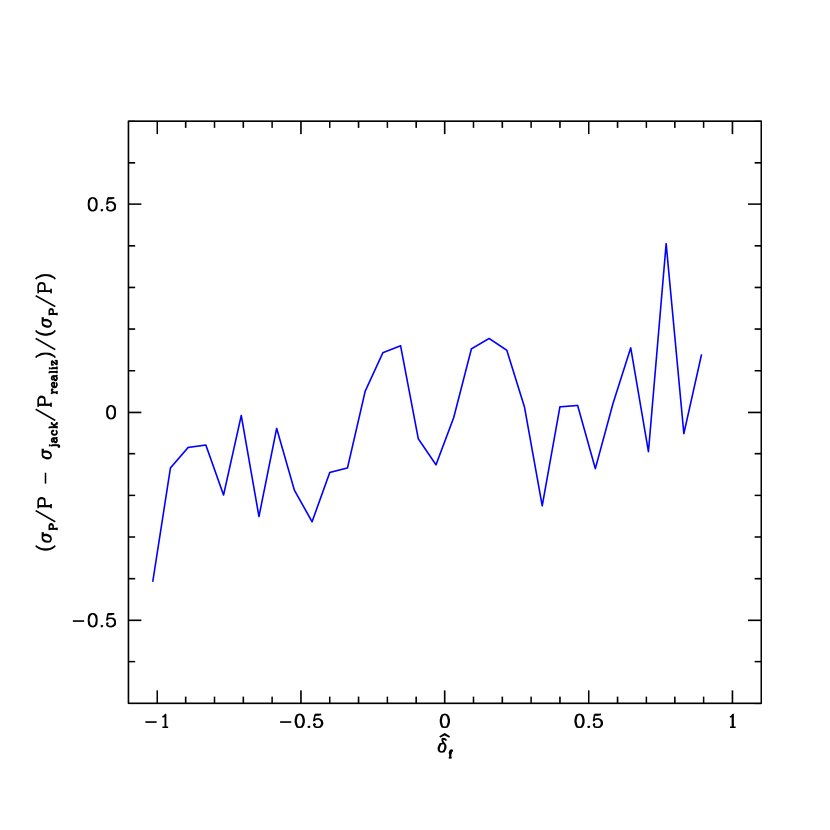
How well does the jackknife technique described above work? In Figure 3 we compare our jackknife estimate of the fractional error on the flux pdf with an estimate from the dispersion across many simulation realizations. The jackknife error estimate is generally good to better than $20\%$, but seems to produce a systematic overestimate of the error at low $\delta_{f}$. The apparent overestimate of the errors is at least conservative in the sense that parameter constraints would only tighten if we were to adopt smaller error bars on these points. On the other hand, the error bars on the points in the high $\delta_{f}$ tail may be underestimated using the jackknife estimator. In this case, there are so few pixels in the high $\delta_{f}$ tail of the pdf that our jackknife method is unreliable. To overcome this difficulty, we again adopt a conservative approach and use the variance measured from the lognormal simulations to represent the variance for the high $\delta_{f}$ bins in our measurement from real data.

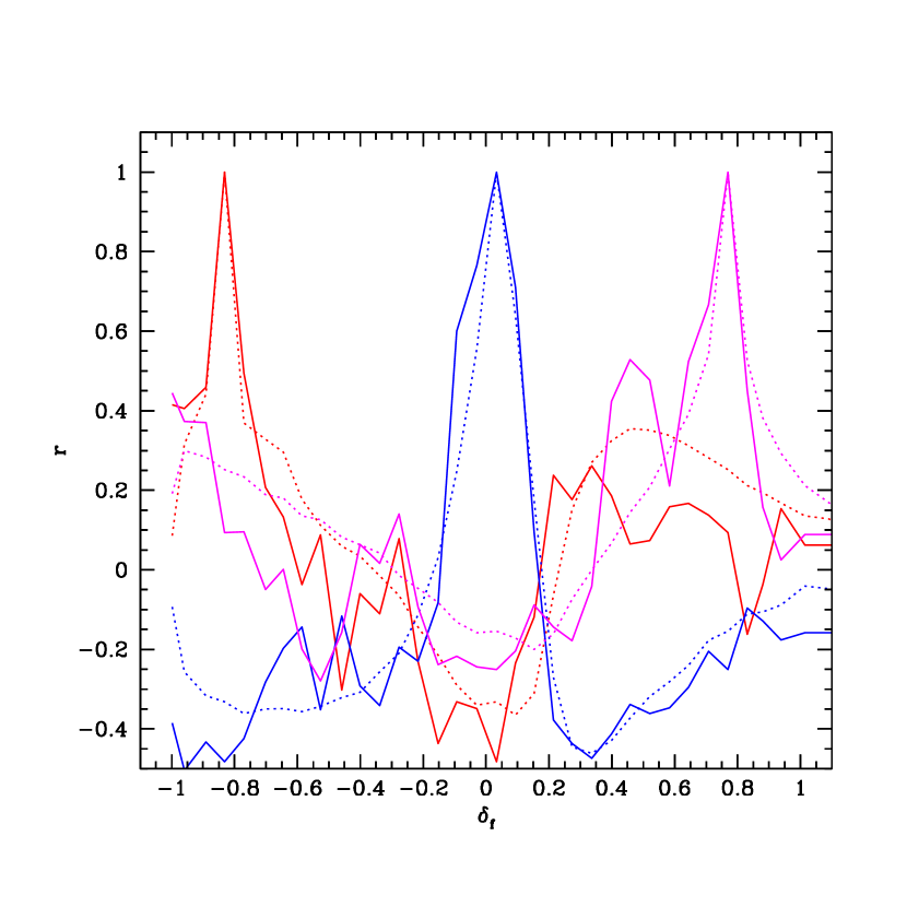
Next, we consider the off-diagonal terms in the covariance matrix. We find that our jackknife estimates of the off-diagonal elements of the covariance matrix are quite noisy. After all, we are attempting to measure $36\times 37/2=666$ matrix elements from only $3499$ data pixels. To get around this difficulty, we first measure the correlation coefficient from many realizations of the mock lognormal spectra. The correlation coefficient is defined by $r(i,j)=Cov(i,j)/\sqrt{Cov(i,i)Cov(j,j)}$. Next we assume that the real data has the same correlation coefficient as the mock data, and estimate the data covariance from the simulated correlation coefficient $r(i,j)$ and the jackknife estimate of the data variance, i.e. $Cov_{\rm d}(i,j)=r_{\rm s}(i,j)\sqrt{Cov_{\rm d}(i,i)Cov_{\rm d}(j,j)}$. Here the subscript ‘d’ indicates a quantity measured from real data, while the subscript ‘s’ represents a quantity measured from the lognormal simulations. This approach allows us to estimate the off-diagonal terms in the data covariance matrix, which are significant, but cannot be estimated cleanly from the data alone. The approach is justified to the extent that the correlation coefficient in the lognormal simulation is representative of the true correlation coefficient in the real data. In Figure 4 we show a comparison of the correlation coefficient measured from the data with a jackknife estimator, which is noisy, and that measured from the lognormal simulations, which is smooth. From the figure, one can see that the simulation measurement is fairly consistent with a smooth version of the noisy jackknife estimate, justifying our approach.

Figure 4.— We show, on the one hand the noisy jackknife estimates of the correlation coefficient from the data (solid lines), and on the other hand, simulation estimates of the correlation coefficient (dotted lines). The red line is the correlation coefficient for a bin with an average flux of $\delta_{f}=-0.832$, the blue line has an average flux of $\delta_{f}=0.0326$, and the magenta line $\delta_{f}=0.769$. The simulation measurements are fairly consistent with a smooth version of the noisy jackknife estimate from real data.

This procedure then provides us with an estimate of the full covariance matrix. There is one last detail that we need to address before proceeding with the remaining analysis. The difficulty is that the flux pdf is required to satisfy a normalization condition, $\int d\delta_{f}P(\delta_{f})=1$, and the data vectors are hence not linearly independent, and the covariance matrix is nearly singular. We therefore diagonalize the covariance matrix, and rebuild it by eliminating the eigenvector with the smallest eigenvalue. In other words, the rebuilt covariance matrix can be written as

$$\tilde{C}_{ij}=\sum_{k=1}^{N_{m}}U_{ik}U_{jk}\lambda_{k},$$ (5)

where $\tilde{C}_{ij}$ is the ‘regularized’ covariance matrix, $U$ is the unitary matrix that diagonalizes the covariance matrix, and $\lambda_{k}$ is the $k$th eigenvalue of the covariance matrix. The eigenvalues are sorted by size, with $\lambda_{1}$ denoting the largest eigenvalue. The sum extends up to $N_{m}=35$, i.e. – $N_{m}$ is the number of bins minus $1$. This ‘regularized’ covariance matrix can then be stably inverted and used to compute $\chi^{2}$ when comparing theoretical models with data (see §4).

Our estimates of the flux pdf and its error bars in the fiducial redshift bin are given in Table 4. The flux pdf and error bars for the other redshift bins (see Table 1) are given in Tables 5–7. In Figure 5 we show our pdf measurement in the different redshift bins. The pdf evolves as one expects – a larger fraction of pixels in the spectrum become opaque with increasing redshift. Tables with the covariance matrices for each redshift bin can be obtained electronically from the website http://t8web.lanl.gov/people/heitmann/lyma/.

Figure 5.— Measured flux pdf in redshift bins with mean redshifts of $\langle z\rangle=2.26,2.72,3.28$, and $3.99$.

With our estimates of the flux pdf and its covariance matrix in hand, we now demonstrate that our estimator satisfies the criteria we described in the beginning of this section. The first criterion, that the estimator be insensitive to the numerical resolution limits of the simulations, is established in the Appendix. The second criterion is clearly satisfied, since the estimator defined in Eqn. (3) does not refer to the unabsorbed continuum level.

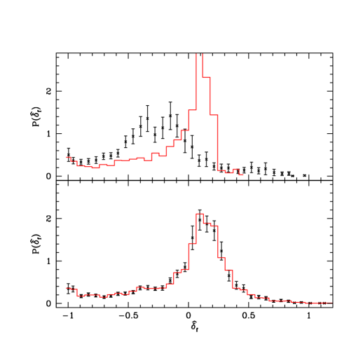
The third criterion, that our estimator is insensitive to the shape of the quasar continuum, is not obvious. In order to investigate this, we estimate the pdf of $\delta_{f}$ from the ‘raw’ data as well as from a version of the data that has first been continuum-normalized, as described in Rauch et al. (1997). If our procedure of applying a large-scale filtering to form $\delta_{f}$ is robust to the unknown continuum shape, then we should get very much the same pdf whether we measure the pdf using the raw data or the continuum-fitted data.

We illustrate our approach in Figure 6 where we measure the pdf of $\delta_{f}$, for each of the raw data and the continuum-fitted data, in two different ways. First, we measure the pdf from each of the raw and the continuum-fitted data, assuming a flat mean. In this case the pdf of $\delta_{f}$ differs substantially between the continuum-fitted and the raw data. The continuum has power on large scales, and the flux pdf will differ significantly between the raw and the continuum-normalized data if we don’t account for this. Second, we measure the pdf from each of the raw and the continuum-fitted data, with $\delta_{f}$ formed using the $R=500$ km/s smoothing to define $\delta_{f}$ as described above. In this case the pdf of $\delta_{f}$ is extremely similar between the continuum-normalized and raw data. In one case we have measured the pdf of $\delta_{f}$ from data that has first been continuum-normalized, and in the second case we did not perform any continuum-normalization, effectively assuming that the continuum is flat. The similarity between the pdf of $\delta_{f}$ under these two very different assumptions regarding the true quasar continuum, demonstrates that the pdf of $\delta_{f}$ is insensitive to our assumptions about the quasar continuum. To provide a quantitative measure of the similarity between the pdf measured in the two different ways, we compute $\chi^{2}$ between the two probability distributions. We find, comparing our $36~{}\delta_{f}$ bins, and including estimates of the off-diagonal elements in the covariance matrix, that $\chi^{2}=8.3$. The pdf of $\delta_{f}$ for the continuum-fitted and raw data are therefore in close agreement.

Figure 6.— Flux pdf from continuum fitted data (red histogram) and from raw data (black points with error bars). The flux pdfs in the top panel are formed assuming a flat mean to estimate $\delta_{f}$, while in the bottom panel $\delta_{f}$ is defined using a large-scale smoothing of $R=500$ km/s. The error bars on the pdf measured from the continuum fitted data, which are comparable to those from the raw data, are not shown for visual clarity. The close agreement between the pdf of the flux field measured from the raw data and that measured from the continuum-fitted data, when both are smoothed on a scale of $R=500$ km/s, illustrates that our procedure is robust to the continuum. The disagreement between the flux pdfs in the top panel, formed assuming a flat mean, is due to large-scale power in the continuum.

4. Constraints on the Mass Power Spectrum using the flux power spectrum and the flux pdf

The next step, after demonstrating that we can measure the flux pdf robustly, is to show that the flux pdf is useful in constraining the mass power spectrum, when employed in conjunction with the flux power spectrum. In particular, we emphasize that the flux pdf is sensitive to $A$, the parameter related to the amplitude of the ionizing background, and hence we can place constraints on the mass power spectrum, without making any assumptions about the mean flux in the Ly$\alpha$ forest.

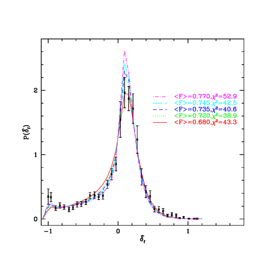
In Figure 7 we show our pdf measurement at $z=2.72$ as well as theoretical predictions for the pdf for the models shown in Figure 1, each of which fits the observed flux power spectrum, in spite of having very different matter power spectra. While the flux pdfs of each model look fairly similar by eye, one can distinguish between them statistically. Of these models, the minimum $\chi^{2}$ obtained from fitting to the PDF alone, occurs at $\langle F/F_{c}\rangle=0.720$, with $\chi^{2}=38.88$. The fit is reasonable given that we compare the theoretical flux pdf with the measured flux pdf for $\sim 34$ degrees of freedom (36 data points - 1 normalization condition - 1 prior on $T_{0}$), and so the fit roughly corresponds to $\chi^{2}/\nu\sim 1.1$, which should be exceeded randomly $\sim 26\%$ of the time. The model with a lower mean flux of $\langle F/F_{c}\rangle=0.680$ is a significantly worse fit with $\chi^{2}=43.26$. Similarly models with significantly higher mean transmitted flux are also poor fits to the data. Specifically, the model with $\langle F/F_{c}\rangle=0.750$ has $\chi^{2}=42.46$, and the model with $\langle F/F_{c}\rangle=0.770$ has $\chi^{2}=52.86$.

The key point is that it is easy to find two models that, while differing significantly in their photo-ionizing backgrounds, yield the same flux power spectrum (and hence have the same variance) – however these two models will generally differ in their higher moments. In particular, the model with $\langle F/F_{c}\rangle=0.680$ has a variance of $\langle\delta_{f}^{2}\rangle=0.134$ and a skewness of $S=\langle\delta_{f}^{3}\rangle/\langle\delta_{f}^{2}\rangle^{3/2}=-0.975$. The model with $\langle F/F_{c}\rangle=0.770$ has a nearly identical variance, but its skewness is rather different, $S=-1.24$. To clarify the situation, let us consider a simplified argument for how the information in the skewness complements the information in the flux power spectrum. The pdf of $\delta_{f}$ is mainly described by two parameters, its variance $\langle\delta_{f}^{2}\rangle$, and its skewness, $S=\langle\delta_{f}^{3}\rangle/\langle\delta_{f}^{2}\rangle^{3/2}$. The underlying model, on the other hand, mainly depends on the variance of the density field, smoothed on some scale, $\langle\delta_{\rho}^{2}\rangle$, and the amplitude of the ionizing background, parameterized by $A$, or effectively $\langle F/F_{c}\rangle$. Now it is easy to imagine that one can adjust $A$ to match the flux variance, $\langle\delta_{f}^{2}\rangle$ for density fields with very different variances, $\langle\delta_{\rho}^{2}\rangle$. However, the skewness depends on the variance of the density field, $\langle\delta_{\rho}^{2}\rangle$, and on $A$ in a different way than the flux variance $\langle\delta_{f}^{2}\rangle$, as one can see in Figures 10-12 of Gaztanaga & Croft (1999). Hence, the information in the skewness provides an effective way of breaking the degeneracy between the amplitude of the ionizing background and the amplitude/slope of the matter power spectrum.

Figure 7.— Flux pdf of the models shown in Figure 1, illustrating that the flux pdf is helpful in breaking the degeneracy between the mean transmission and the amplitude/slope of the mass power spectrum. One should keep in mind that the error bars in different $\delta_{f}$ bins are correlated.

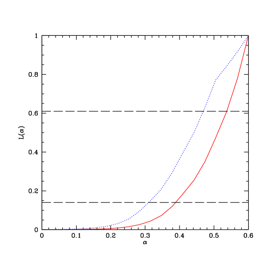
Having demonstrated the sensitivity of the flux pdf to $\langle F/F_{c}\rangle$, we constrain $\langle F/F_{c}\rangle$ at $z=2.72$ by marginalizing over all of the other parameters. The results are shown in Figure 8, the reduced likelihood function for $\langle F/F_{c}\rangle$ using joint constraints from the flux power spectrum and the flux pdf. The allowed 1-$\sigma$ range is $\langle F/F_{c}\rangle=0.730+0.007-0.027$, while the allowed 2-$\sigma$ range is $\langle F/F_{c}\rangle=0.730+0.014-0.038$. The quoted central value, $\langle F/F_{c}\rangle=0.730$, corresponds to the mean transmitted flux that maximizes the likelihood function. The reduced likelihood function with the current data set is hence rather broad, only weakly constraining values of the mean transmitted flux less than our central value. However, we reiterate that our constraints on the mean transmitted flux do not rely on ‘continuum fitting’ and are completely independent of the usual measurements. Next we compare our constraints with the priors adopted on the mean transmitted flux in the Ly$\alpha$ forest adopted by other authors. The prior adopted by Croft et al. (2002) is $\langle F/F_{c}\rangle=0.705\pm 0.012$, the prior of Viel et al. (2004b) is $\langle F/F_{c}\rangle=0.730\pm 0.011$, and SMM03 consider two priors on the mean transmitted flux: $\langle F/F_{c}\rangle=0.742\pm 0.012$, and one with expanded error bars, $\langle F/F_{c}\rangle=0.742\pm 0.027$. Our results are thus intermediate between the Croft et al. (2002) prior and the SMM03 prior, and do not strongly constrain either possibility. From Figure 8, one can see, however, that our constraint is narrower than the prior adopted by SMM03.

Figure 8.— Reduced likelihood function for the mean flux, $\langle F/F_{c}\rangle$, marginalized over all of the other parameters at $z=2.72$. The solid red line is our constraint from combining the flux pdf with the flux power spectrum. The green dotted line is the ‘expanded error’ prior suggested by SMM03, based on local continuum-fitting estimates of the mean transmitted flux. The black short-dashed line is the prior adopted by Croft et al. (2002) based on the PRS measurements of the mean transmitted flux. The blue long-dashed line is the prior adopted by Viel et al. (2004) based on their own local continuum-fitting estimates of the mean transmitted flux.

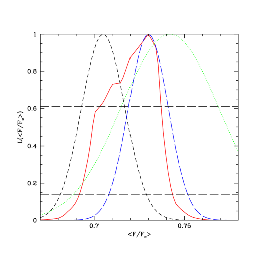
These constraints are conservative in the sense that we assume very little about the shape and amplitude of the linear matter power spectrum. We can turn things around by requiring $\Lambda$CDM and examining how tight the constraints on the mean transmitted flux become. Specifically, we adopt a $5\%$ prior on the slope of the linear power spectrum, and a $10\%$ prior on the amplitude of the linear power spectrum, centered around a scale-invariant model with $\sigma_{8}(z=0)=0.9$. The constraint on the mean transmission (2-$\sigma$) in the Ly$\alpha$ forest becomes $\langle F/F_{c}\rangle=0.724\pm 0.012$. This can be compared to the (2-$\sigma$) constraint we obtain without any prior on the matter power spectrum, $\langle F/F_{c}\rangle=0.730+0.014-0.038$. The prior on the matter power spectrum thus disfavors the very small values of the mean transmission that are allowed without the prior.

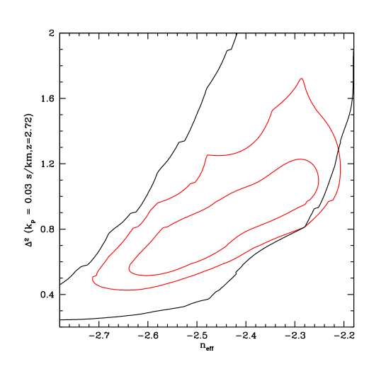
How tight do the constraints on the slope and the amplitude of the mass power spectrum become, when assuming nothing about the mean transmission but using the flux pdf? In Figure 9 we show the constraint on the mass power spectrum amplitude and slope using the information from both the flux pdf and the flux auto spectrum. One can see that while the constraints on the mass power spectrum amplitude and slope are still fairly weak, using the flux pdf as well as the auto spectrum significantly tightens the constraints. The flux pdf disfavors the high values of the mean transmitted flux that fit the flux power spectrum with high amplitude mass power spectrum normalizations. The information in the flux pdf thereby helps to break the degeneracy between the mean transmitted flux and the mass power spectrum normalization/slope by tightening constraints on the mean transmitted flux. In the Appendix we estimate the systematic error on our constraints resulting from the limited resolution of our simulations.

Figure 9.— The red contours show 1- and 2-$\sigma$ constraints on the mass power spectrum using both the probability distribution function of $\delta_{f}$ and the auto spectrum, without assuming any prior on the mean transmitted flux in the Ly$\alpha$ forest. The black contour shows the 2-$\sigma$ constraint on the matter power spectrum using only the auto spectrum, without enforcing any prior on $\langle F/F_{c}\rangle$.

5. Constraints on the Slope of the Temperature-Density Relation

In this section we illustrate that our measurement of the flux pdf also yields a constraint on the slope of the temperature-density relation, $\alpha$, at $z=2.72$. The relation between flux and density depends on the slope of the temperature-density relation [Eqn. (1)]. We find that, when all of the other modeling parameters are fixed, the probability of a pixel having no Ly$\alpha$ absorption becomes smaller as $\alpha$ increases (Gaztanaga & Croft 1999). This distinction is somewhat washed out by the smoothing we apply to the spectra. In spite of this we still find a constraint on the slope of the temperature-density relation, $\alpha$. In Figure 10, we show the reduced likelihood function for the parameter $\alpha$ obtained by marginalizing over all of the other parameters. From the figure one can see that $\alpha\gtrsim 0.4$ is required by our measurements at the 2-$\sigma$ level. We checked that this constraint does not depend significantly on our assumed prior on the temperature at mean density, $T_{0}=300\pm 50$ (km/s)². Relaxing this prior, the constraint only weakens to requiring $\alpha\gtrsim 0.32$ at 2-$\sigma$. This constraint is surprising if HeII is reionized at redshifts slightly larger than $z\sim 2.72$, in which case we expect the slope of the temperature-density relation to be close to isothermal (Hui & Gnedin 1997). We caution however, that we only considered one thermal history in calculating the gas pressure smoothing in our HPM simulations. Desjacques & Nusser (2004) find that the effect of varying the amount of gas pressure smoothing on the statistics of the Ly$\alpha$ forest is degenerate with the effect of varying the slope of the temperature-density relation. Our constraint on the temperature-density relation is likely to weaken if we properly marginalize over the amount of gas pressure smoothing.

Figure 10.— Reduced likelihood function for the slope of the temperature density relation, $\alpha$. The red solid line shows the likelihood function for $\alpha$ from comparing theoretical models with the observed flux power spectrum and flux pdf at $z=2.72$. The blue dotted line illustrates that our results only weaken slightly if we relax our adopted prior on the temperature at mean density.

6. Discussion

In this paper we have demonstrated that the information in the flux pdf, when used in conjunction with the flux power spectrum, can tighten constraints on the matter power spectrum. In particular, the flux pdf of $\delta_{f}$ is robust to our treatment of the quasar continuum, yet sensitive to the amplitude of the photo-ionizing background, a sensitivity that allows us to break degeneracies between the matter power spectrum and the amplitude of the ionizing background. Hence, we can constrain the matter power spectrum without relying on measurements of the mean transmitted flux which depend on estimating the normalization of the quasar continuum.

It is appropriate to consider the prospects for using this methodology to obtain tighter constraints on cosmology and the physics of the IGM in the future, especially since our present constraints are still quite weak. Observationally, the pdf of $\delta_{f}$ can be measured with very high statistical precision using the SDSS (Burgess, Burles et al., 2005, in prep.). Theoretically, two main improvements can be expected. First, we will soon be able to simulate the same cosmological volume at higher resolution. This will allow us to utilize the small-scale information obtained in the flux power spectrum and the flux pdf and eliminate systematic errors due to poor resolution. Second, our pseudo-hydrodynamic approach should be compared systematically with full hydrodynamic simulations (Gnedin & Hui 1998, Meiksin & White 2001, McDonald 2004b, Viel et al. 2005b). Alternatively, it may be feasible to run a grid of fully hydrodynamic simulations in the near future.

There are a few other issues that would be interesting to pursue. First, the methodology described here can be applied at a range of redshifts to constrain the evolution of the slope of the temperature density relation, the mean transmitted flux and the amplitude of the ionizing background, as well as the slope and amplitude of the linear matter power spectrum. Our methodology may actually be most useful at high redshift, where we did not compare our measurements with theoretical models. At high redshift, continuum-fitting should be most problematic since there are then zero, or very few, unabsorbed regions of spectra with which to define the continuum. Applying our method over a range of redshifts would also provide constraints on the evolution of the linear matter power spectrum with redshift, offering a test of the extent to which the structure in the Ly$\alpha$ forest is governed by gravitational instability (Croft et al. 2002). Second, the probability distribution of $\delta_{f}$ might be useful in constraining primordial non-gaussianity (Gaztanaga & Croft 1999). Third, we can generalize our measurements to examine the pdf as a function of smoothing scale. Finally, the flux pdf might be useful in constraining the impact of non-gravitational processes on the Ly$\alpha$ forest. Gravitational instability makes definite predictions for the relationship between the variance of the density field and its higher order moments – to the extent that the Ly$\alpha$ forest is dominated by gravitational instability, these scalings should be imprinted on the flux statistics in the Ly$\alpha$ forest (Zaldarriaga et al. 2001b, Fang & White 2004). The good agreement of our measured flux pdf and simulations should therefore imply a constraint on feedback processes.

Appendix

The primary purpose of this section is to examine the sensitivity of our results to limitations in our simulation box size and resolution. The $\Lambda$CDM simulations in this paper use $512^{3}$ baryons and $512^{3}$ dark matter particles, with $512^{3}$ mesh points, in a $40$ Mpc/$h$ box. The simulations were run with a fast, parallel N-body code, MC² (Mesh-based Cosmology Code). MC² was recently extensively tested against five other state-of-the-art codes (Heitmann et al. 2004). A detailed description of the code will be given in Habib et al. (2005) (in preparation), including a description of our implementation of HPM, the pseudo-hydrodynamic method of Gnedin & Hui (1998). Our implementation differs from that of Gnedin & Hui (1998) in that we follow separately two particle species: baryonic particles that experience gas forces as well as gravity, and dark matter particles that interact only gravitationally. We adopt the input transfer function of Hu and Sugiyama (1996) with cosmological parameters of $\Omega_{m}=0.3,\Omega_{\Lambda}=0.7,\Omega_{b}h^{2}=0.02$. Simulations with differing spectral indices, $n$, are each normalized so as to have the same amplitude, $\Delta^{2}(\tilde{k}_{p},z)$, on the scale $\tilde{k}_{p}=0.008$ s/km at a redshift of $z=3$. The output with $n=1.0$ has a normalization given by $\sigma_{8}(z=0)=0.84$. Finally, we need to specify the thermal history of the IGM in order to compute the gas pressure term in our HPM simulation. We adopt a similar thermal history to that adopted in McDonald & Miralda-Escudé (2001). Specifically, we assume that $T_{0}$ is $25,000$ K and that the slope of the temperature-density relation is $\alpha=0$ at a reionization redshift of $z_{\rm reion}=10$, while $T_{0}=18,000$ K and $\alpha=0.3$ at $z=4$. We linearly interpolate between these values to specify the gas pressure at intermediate redshifts, and use the $z=4$ values at lower redshifts. While the true thermal history of the IGM may be rather different than this simple model, we find that the flux power spectrum on the large scales considered in this paper, $k\lesssim 0.02$ s/km, are relatively insensitive to the thermal history. More systematic tests of the dependence of our results on thermal history are clearly warranted, however.

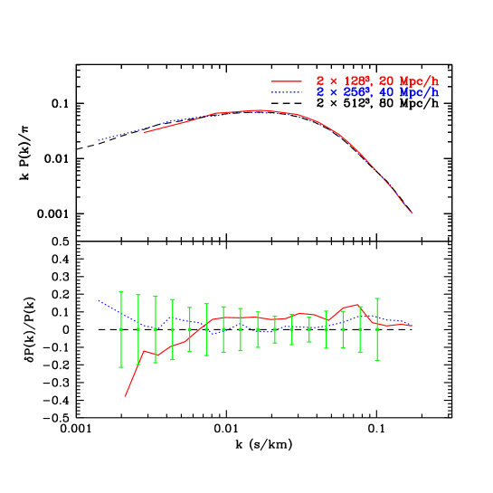
In Figure 11, we show flux power spectrum measurements at $z=3$ for simulations with box sizes of $20,40$ and $80$ Mpc/$h$. Each simulation has a resolution equivalent to that of a $2\times 512^{3}$ particle, $80$ Mpc/$h$ simulation. For the purpose of testing the resolution and box size of our simulations, we generate flux fields at $z=3.0$ for a model with $(a,n,k_{f},T_{0},\alpha,\langle F/F_{c}\rangle)=(0.2480,1.0,300$ (km/s)², $0.4,0.684).$ For this model, the box size convergence test shown in the figure indicates that any difference in the flux power spectrum between the $40$ Mpc/$h$ simulation and the $80$ Mpc/$h$ is at most comparable to the (1-$\sigma$) statistical error on the Croft et al. (2002) measurement, and always less than the 2-$\sigma$ statistical errors shown in the figure. Furthermore, much of the difference between the $40$ Mpc/$h$ simulation and the $80$ Mpc/$h$ simulation is likely random, as opposed to systematic, owing simply to differences in the random initial conditions adopted in the two simulations. Therefore, a $40$ Mpc/$h$ simulation box is adequate to achieve convergence at the level of the Croft et al. (2002) error bars.

Figure 11.— Convergence test of the flux power spectrum with box size at $z=3.0$. In the top panel, we show the flux auto spectrum in $20,40$ and $80$ Mpc/$h$ simulation boxes. Each model has the same resolution, corresponding to $2\times 128^{3}$, $2\times 256^{3}$, and $2\times 512^{3}$ particles, respectively. The model is described by $(a,n,T_{0},\alpha,\langle F/F_{c}\rangle)=(0.2480,1.00,300$ (km/s)², $0.4,0.684).$ The bottom panel shows the fractional difference between the flux power spectrum in each of the $20$ and $40$ Mpc/$h$ simulation boxes with that in the $80$ Mpc/$h$ simulation box. The green points show the size of the (2-$\sigma$) fractional error bars from Croft et al. (2002) at $z=2.72$.

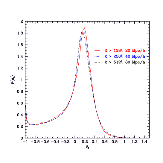
In Figure 12, we show the equivalent convergence test for the flux pdf. In particular, it is important to confirm that our results converge with box size, in spite of the size we choose for our large-radius filter, $R=500$ km/s, which is roughly 1/8th the size of the $40$ Mpc/$h$ simulation box. The figure illustrates that any difference between the flux pdf in a $40$ Mpc/$h$ simulation box and that in a $80$ Mpc/$h$ simulation box is very small.

Figure 12.— Convergence test of the flux pdf with box size at $z=3.0$. The simulation flux fields have been smoothed with filters of $R=500$ km/s and $r=30$ km/s. The flux pdf is shown in simulation boxes of size $20,40$ and $80$ Mpc/$h$, each with the same resolution.

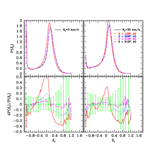
Another important aspect of our modeling is the choice of the smoothing scale, $r$, at which we smooth the data and simulated spectra in order to measure the pdf of $\delta_{f}$. We aim to choose this scale to be sufficiently large that we can guarantee the convergence of the flux pdf, when the flux fields are smoothed on the scale $r$, with increasing resolution. To test the convergence of the flux pdf with resolution we have generated the flux pdf assuming a range of different small-scale smoothings, $r$, in simulations of varying resolution. (The varying resolution simulations are described in more detail below.) In Figure 13 we show the convergence of our simulation measurements with increasing resolution for small-scale smoothings of $r=5$ km/s and $r=30$ km/s. As expected, the convergence is better in the case of the $r=30$ km/s filter than in the case of the $r=5$ km/s filter. In the case of the $r=30$ km/s filter it is clear that the convergence of our results is adequate for our present data sample. The convergence also appears surprisingly good in the case of the $r=5$ km/s filter: the difference between the $256^{3}$, $40$ Mpc/$h$ and the $512^{3}$, $40$ Mpc/$h$ simulation is only slightly larger than the statistical error bars. However, in our present analysis we conservatively adopt the $r=30$ km/s filter.

Figure 13.— Convergence test of the flux pdf with resolution at $z=3.0$. We show the flux pdf in a $40$ Mpc/$h$ simulation box for simulations with $2\times 128^{3}$, $2\times 256^{3}$, and $2\times 512^{3}$ particles, as well as the flux pdf in a $60$ Mpc/$h$ simulation with $2\times 512^{3}$ particles. The panels on the left side show the flux pdf for a small-scale smoothing of $r=5$ km/s and the panels on the right hand side show the flux pdf for a small-scale smoothing of $r=30$ km/s. In each case the flux fields were smoothed with the same large radius filter of $R=500$ km/s. The top panels show the measurements themselves, while the bottom panels show the fractional difference between the lower resolution measurements and the high resolution measurement. The green points represent the approximate (1-$\sigma$) fractional error from the present data sample.

Next, we examine the convergence of the flux power spectrum with resolution. To perform this test, we measure the flux power spectrum for several simulations of the same box size, but differing particle number. Specifically, we measure the flux power spectrum in $40$ Mpc/$h$ simulations with each of $2\times 128^{3},2\times 256^{3}$ and $2\times 512^{3}$ particles. Each of the $40$ Mpc/$h$ simulations are generated with similar initial conditions: the initial conditions for, e.g., the $2\times 256^{3}$ simulation are generated by averaging the initial conditions for the $2\times 512^{3}$ particle simulation over every eight particles. We also generate a $2\times 512^{3}$ particle, $60$ Mpc/$h$ simulation to further illustrate the convergence of our results with varying mesh size. This simulation is generated with different initial conditions than that of the $40$ Mpc/$h$ simulations, but Figure 11 demonstrates that the resulting random differences between the flux power spectra should be small for the $k$-modes of interest, $k\gtrsim 0.01$ s/km. Finally, we extrapolate our results to the case of infinite resolution using Richardson extrapolation. We make this extrapolation in two ways. First we assume that the convergence of the flux power spectrum for a given $k$-mode is linear in the mesh size, and second we assume that the convergence is quadratic in the mesh size. The results of our resolution test are shown in Figure 14. Interestingly, the convergence appears better in the flux pdf than in the auto spectrum, although this is partly due to the large error bars on the pdf measurement; our pdf estimate comes from a smaller data sample than the sample Croft et al. (2002) use to estimate the flux power spectrum. At any rate, the test shows rather large systematic differences between the lowest resolution simulation, with $2\times 128^{3}$ particle and the $2\times 512^{3}$ particle, $40$ Mpc/$h$ simulation. These differences are expected since the lowest resolution simulations do not resolve the gas pressure smoothing scale. The measurements made using the $2\times 256^{3}$, $40$ Mpc/$h$ simulation and the $2\times 512^{3}$, $60$ Mpc/$h$ simulation are substantially closer to those from the $2\times 512^{3}$, $40$ Mpc/$h$ simulation.

Figure 14.— Convergence test of the flux auto spectrum with resolution at $z=3.0$. We show the flux auto spectrum in a $40$ Mpc/$h$ simulation box for each of $2\times 128^{3},2\times 256^{3}$, and $2\times 512^{3}$ particles. We also show the flux auto spectrum in a $2\times 512^{3}$ particle, $60$ Mpc/$h$ simulation box, and two extrapolations of the flux auto spectrum to infinite resolution. In one extrapolation we assume that the flux power in each $k$-mode converges linearly with the mesh size, and in the other extrapolation we assume that the flux power converges quadratically with the mesh size. The top panel shows the flux power, while the bottom panel shows the fractional difference with the $512^{3}$, $40$ Mpc/$h$ simulation. The green points show the size of the (2-$\sigma$) fractional error bars from Croft et al. (2002) at $z=2.72$. In our present analysis, we only include measurements on scales larger than that indicated by the vertical dashed line.

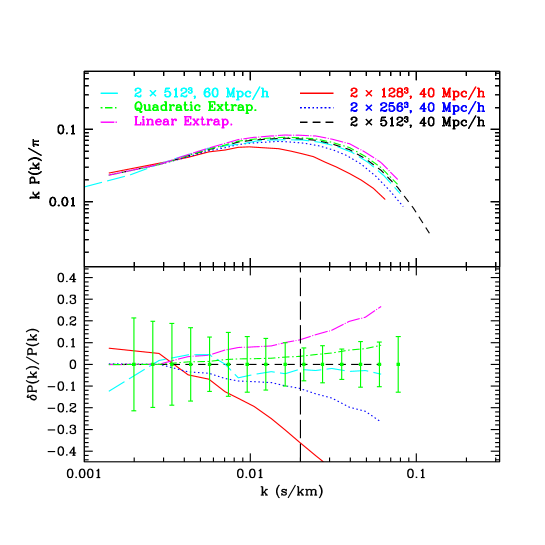
How close is the flux power spectrum in our $512^{3}$, $40$ Mpc/$h$ simulation to what we would measure from an infinite resolution simulation? This depends, of course, on how we extrapolate our measurements to infinite resolution. If the convergence is as good as quadratic in the mesh size, then our present simulations are adequate: any systematic difference between the $2\times 512^{3}$, $40$ Mpc/$h$ simulation and the quadratic extrapolation to perfect resolution is small compared to the statistical error bars on the Croft et al. (2002) measurement. However, if the convergence is only linear in the mesh size, then the figure illustrates that, even limiting our analysis to scales of $k\lesssim 0.02$ s/km, we are making some non-negligible systematic error. Specifically, assuming linear convergence, our $2\times 512^{3}$, $40$ Mpc/h flux power spectrum is good to $\sim 10\%$. While this convergence appears to be quite acceptable, it is in fact comparable to the 2-$\sigma$ statistical error on the Croft et al. (2002) measurement at $z=2.72$. It is important to decide which is a more accurate description of the convergence of our results with mesh size: linear or quadratic convergence? At present, the best we can do to answer this question is to ask how well we can predict the results of the $2\times 512^{3},40$ Mpc/$h$ simulation by extrapolating from the lower resolution simulations. On this basis, we find that neither linear nor quadratic convergence is a good description over the full range of $k$-modes we consider. At the $k$-modes that our most important for our convergence study, $k\sim 0.02$ s/km, by making the (worse-case) assumption that linear convergence is an accurate description, we can check how large a systematic error we are possibly making due to imperfect simulation resolution.

Figure 15.— An estimate of the systematic error in our constraints on the linear matter power spectrum owing to the imperfect resolution of our numerical simulations. The black contours indicate 1- and 2-$\sigma$ constraints on the slope and amplitude of the linear matter power spectrum. The red contours are estimates of the same constraints we expect given infinite resolution simulations.

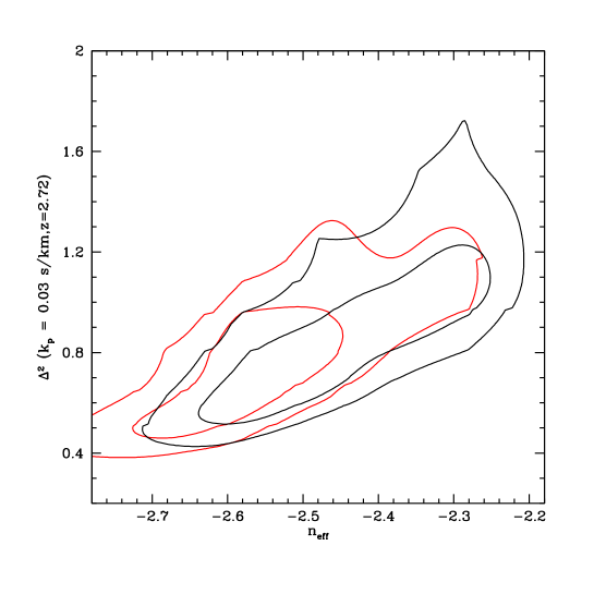
In order to gauge the importance of any systematic error from the limited resolution of our simulations we do the following check. We assume that the convergence of our flux power spectrum measurement is linear in the mesh size, and derive a correction factor at each $k$-mode by dividing the linearly-extrapolated flux power by that in our $2\times 512^{3}$ particle, $40$ Mpc/$h$ simulation box (see also McDonald et al. 2004b). Assuming that this correction factor is model-independent, we then multiply each model in our grid by this correction and examine how much our constraints on the slope and amplitude of the matter power spectrum change. This is clearly an imperfect procedure: the relevant correction factor is likely model-dependent and our assumption of linear convergence is not strongly established. In spite of these uncertainties, this test gives some indication of how much our results might change with improved resolution. This is shown in Figure 15, where the black contours show our current constraints, and the red contours indicate our estimate of the same constraints given simulations of infinite resolution. From this plot, the main effect of our limited resolution appears to be to a systematic shift in the inferred slope of the matter power spectrum towards steeper slopes by $\sim 0.1$. The ‘resolution corrected’ contours are also less elongated towards large matter power spectrum amplitudes. From this test, the effect of limited resolution appears to be most degenerate with the slope of the matter power spectrum (see also SMM03). While our present constraints are weak, it is clear that higher resolution simulations will be necessary to obtain more precise constraints in the future.

Table 2Quasar Spectra and Wavelength Range used in the PDF Measurement

Quasar Spectrum	$z_{\rm em}$	$\lambda_{\rm low}(\AA)$	$\lambda_{\rm high}(\AA)$
Q2343+123	2.52	3922.0	3926.6
		3929.3	3966.5
		3970.5	3996.3
		4000.5	4053.2
		4060.6	4077.
		4097.	4108.8
Q1442+293	2.67	3764.4	4089.5
		4095.1	4100.2
		4105.5	4156.2
		4204.5	4250.0
		4336.8	4375.5
		4379.6	4409.28
Q1107+485	3.00	4233.0	4261.3
		4262.7	4306.1
		4308.8	4364.7
		4365.4	4408.5
		4409.5	4434.5
		4437.5	4444.8
		4446.5	4485.7
		4491.9	4534.8
		4541.9	4549.4
		4550.9	4656.3
		4660.3	4670.1
		4678.9	4698.2
		4701.3	4741.3
		4744.9	4797.9
Q1425+604	3.20	4314.0	4320.7
		4321.9	4373.0
		4375.5	4462.5
		4467.5	4486.0
		4490.6	4492.3
		4502.7	4546.0
		4571.9	4591.3
		4593.8	4599.0
		4603.5	4606.6
		4753.9	4821.1
		4829.0	4858.1
		4862.3	4905.4
		4910.0	4916.3
		4918.0	4980.5
		4996.9	5032.0
Q1422+230	3.62	4738.1	4786.4
		4818.0	4884.5
		4885.7	4890.6
		4892.2	4980.7
		4982.2	5002.3
		5003.7	5224.3
		5225.8	5287.3
		5288.5	5364.6
		5369.0	5472.4
		5477.0	5523.0

Note. — Table continued on the next page. The quasar spectra used in the pdf measurement. The wavelength range specified indicates the pixels that are used in the analysis, other data are excluded due to the expected existence of metal lines, damped lyman-alpha systems, or spurious pixels. See also Rauch et al. (1997) and McDonald et al. (2000).

Table 3Quasar Spectra and Wavelength Range used in the PDF Measurement (continued)

Quasar Spectrum	$z_{\rm em}$	$\lambda_{\rm low}(\AA)$	$\lambda_{\rm high}(\AA)$
Q000-262	4.11	5600.0	5637.0
		5639.8	5704.4
		5706.4	5715.2
		5718.2	5724.9
		5727.2	5813.5
		5815.3	5859.7
		5860.8	5953.5
		5956.4	6092.0
Q2237-061	4.55	5692.0	5703.8
		5705.0	5747.4
		5749.7	5774.4
		5774.8	5803.3
		5805.7	5815.3
		5817.6	5830.4
		5831.5	5876.9
		5878.1	5891.1
		5892.0	5897.0
		5898.0	5967.0
		5967.2	5974.8
		5975.6	6020.1
		6020.8	6034.6
		6036.5	6042.7
		6055.5	6063.4
		6068.9	6100.0
		6250.0	6251.6
		6255.4	6282.3
		6290.3	6314.5
		6315.5	6330.6
		6332.3	6402.3
		6405.8	6482.3
		6485.8	6502.0
		6503.5	6549.1
		6550.0	6582.1
		6582.2	6600.0

Note. — Table continued from the previous page. The quasar spectra used in the pdf measurement. The wavelength range specified indicates the pixels that are used in the analysis, other data are excluded due to the expected existence of metal lines, damped lyman-alpha systems or spurious pixels. See also Rauch et al. (1997) and McDonald et al. (2000).

Table 4 The probability distribution of $\delta_{f}$ at $\langle z\rangle=2.72$.

Bin No.	$\delta_{f}$	$P(\delta_{f})$	$\sigma^{2}_{P}(\delta_{f})$	Bin No.	$\delta_{f}$	$P(\delta_{f})$	$\sigma^{2}_{P}(\delta_{f})$
1	-0.9983E+00	0.3483E+00	0.1406E-01	19	0.9415E-01	0.1964E+01	0.5558E-01
2	-0.9596E+00	0.3390E+00	0.4917E-02	20	0.1526E+00	0.1872E+01	0.3540E-01
3	-0.8913E+00	0.1718E+00	0.1371E-02	21	0.2142E+00	0.1714E+01	0.5379E-01
4	-0.8317E+00	0.2090E+00	0.1600E-02	22	0.2739E+00	0.1235E+01	0.4550E-01
5	-0.7706E+00	0.1858E+00	0.1213E-02	23	0.3366E+00	0.6548E+00	0.1588E-01
6	-0.7013E+00	0.1486E+00	0.1105E-02	24	0.3985E+00	0.4273E+00	0.8478E-02
7	-0.6450E+00	0.1765E+00	0.9211E-03	25	0.4584E+00	0.3530E+00	0.7458E-02
8	-0.5853E+00	0.2276E+00	0.1547E-02	26	0.5206E+00	0.1533E+00	0.1817E-02
9	-0.5259E+00	0.2322E+00	0.1491E-02	27	0.5837E+00	0.1486E+00	0.1890E-02
10	-0.4593E+00	0.2647E+00	0.1542E-02	28	0.6443E+00	0.1207E+00	0.1695E-02
11	-0.4016E+00	0.3669E+00	0.2094E-02	29	0.7081E+00	0.5109E-01	0.5303E-03
12	-0.3379E+00	0.3715E+00	0.2788E-02	30	0.7693E+00	0.6966E-01	0.7736E-03
13	-0.2766E+00	0.3437E+00	0.1596E-02	31	0.8312E+00	0.5109E-01	0.7147E-03
14	-0.2161E+00	0.3622E+00	0.2797E-02	32	0.8806E+00	0.1393E-01	0.6471E-04
15	-0.1519E+00	0.5387E+00	0.3878E-02	33	0.9382E+00	0.2322E-01	0.2808E-03
16	-0.9288E-01	0.6966E+00	0.7684E-02	34	0.1014E+01	0.4644E-02	0.3863E-04
17	-0.2913E-01	0.8545E+00	0.1101E-01	35	0.1091E+01	0.4644E-02	0.2454E-04
18	0.3326E-01	0.1547E+01	0.7748E-01	36	0.1130E+01	0.4644E-02	0.9799E-04

Table 5 The probability distribution of $\delta_{f}$ at $\langle z\rangle=2.26$.

Bin No.	$\delta_{f}$	$P(\delta_{f})$	$\sigma^{2}_{P}(\delta_{f})$	Bin No.	$\delta_{f}$	$P(\delta_{f})$	$\sigma^{2}_{P}(\delta_{f})$
1	-0.1015E+01	0.1382E+00	0.5478E-02	19	0.8905E-01	0.2683E+01	0.1241E+00
2	-0.9534E+00	0.1219E+00	0.2655E-02	20	0.1557E+00	0.1894E+01	0.5844E-01
3	-0.8912E+00	0.2032E+00	0.8366E-02	21	0.2122E+00	0.1528E+01	0.8463E-01
4	-0.8349E+00	0.1138E+00	0.1236E-02	22	0.2716E+00	0.8292E+00	0.3612E-01
5	-0.7647E+00	0.1382E+00	0.1511E-02	23	0.3373E+00	0.2764E+00	0.9017E-02
6	-0.7096E+00	0.1382E+00	0.1374E-02	24	0.3928E+00	0.1707E+00	0.8643E-02
7	-0.6471E+00	0.1301E+00	0.1234E-02	25	0.4600E+00	0.9755E-01	0.3620E-02
8	-0.5816E+00	0.1301E+00	0.1092E-02	26	0.5145E+00	0.1219E+00	0.8451E-02
9	-0.5251E+00	0.1301E+00	0.1057E-02	27	0.5767E+00	0.9755E-01	0.4756E-02
10	-0.4579E+00	0.1707E+00	0.1856E-02	28	0.6210E+00	0.8129E-02	0.6836E-04
11	-0.4060E+00	0.2114E+00	0.1800E-02	29	0.0000E+00	0.0000E+00	0.0000E+00
12	-0.3429E+00	0.1707E+00	0.1859E-02	30	0.0000E+00	0.0000E+00	0.0000E+00
13	-0.2701E+00	0.2520E+00	0.3739E-02	31	0.0000E+00	0.0000E+00	0.0000E+00
14	-0.2121E+00	0.3821E+00	0.5326E-02	32	0.0000E+00	0.0000E+00	0.0000E+00
15	-0.1502E+00	0.4796E+00	0.4609E-02	33	0.0000E+00	0.0000E+00	0.0000E+00
16	-0.9019E-01	0.7560E+00	0.2314E-01	34	0.0000E+00	0.0000E+00	0.0000E+00
17	-0.2765E-01	0.1366E+01	0.5216E-01	35	0.0000E+00	0.0000E+00	0.0000E+00
18	0.3238E-01	0.3512E+01	0.3496E+00	36	0.0000E+00	0.0000E+00	0.0000E+00

Table 6 The probability distribution of $\delta_{f}$ at $\langle z\rangle=3.28$.

Bin No.	$\delta_{f}$	$P(\delta_{f})$	$\sigma^{2}_{P}(\delta_{f})$	Bin No.	$\delta_{f}$	$P(\delta_{f})$	$\sigma^{2}_{P}(\delta_{f})$
1	-0.9947E+00	0.2902E+00	0.1450E-01	19	0.9358E-01	0.1049E+01	0.2613E-01
2	-0.9543E+00	0.4551E+00	0.8468E-02	20	0.1538E+00	0.1194E+01	0.2766E-01
3	-0.8906E+00	0.4353E+00	0.2913E-02	21	0.2154E+00	0.1372E+01	0.5276E-01
4	-0.8287E+00	0.3232E+00	0.5159E-02	22	0.2761E+00	0.1200E+01	0.1899E-01
5	-0.7692E+00	0.3034E+00	0.2115E-02	23	0.3388E+00	0.9695E+00	0.1769E-01
6	-0.7084E+00	0.3100E+00	0.2483E-02	24	0.3984E+00	0.7584E+00	0.1251E-01
7	-0.6432E+00	0.3166E+00	0.3222E-02	25	0.4634E+00	0.6529E+00	0.1901E-01
8	-0.5831E+00	0.2704E+00	0.1906E-02	26	0.5220E+00	0.4221E+00	0.4633E-02
9	-0.5225E+00	0.2770E+00	0.2094E-02	27	0.5860E+00	0.2770E+00	0.4519E-02
10	-0.4599E+00	0.3363E+00	0.3365E-02	28	0.6418E+00	0.3297E+00	0.6822E-02
11	-0.4017E+00	0.3891E+00	0.2566E-02	29	0.7016E+00	0.1451E+00	0.3897E-02
12	-0.3419E+00	0.4023E+00	0.2653E-02	30	0.7641E+00	0.7914E-01	0.1172E-02
13	-0.2799E+00	0.4814E+00	0.4446E-02	31	0.8174E+00	0.1319E-01	0.8699E-04
14	-0.2151E+00	0.4155E+00	0.4118E-02	32	0.9020E+00	0.3957E-01	0.5024E-03
15	-0.1488E+00	0.4814E+00	0.3175E-02	33	0.9599E+00	0.6595E-01	0.1799E-02
16	-0.9270E-01	0.6265E+00	0.4565E-02	34	0.1018E+01	0.1978E-01	0.3634E-03
17	-0.2955E-01	0.6925E+00	0.6691E-02	35	0.1087E+01	0.3957E-01	0.2377E-03
18	0.3172E-01	0.7848E+00	0.1571E-01	36	0.1140E+01	0.3297E-01	0.1672E-02

Table 7 The probability distribution of $\delta_{f}$ at $\langle z\rangle=3.99$.

Bin No.	$\delta_{f}$	$P(\delta_{f})$	$\sigma^{2}_{P}(\delta_{f})$	Bin No.	$\delta_{f}$	$P(\delta_{f})$	$\sigma^{2}_{P}(\delta_{f})$
1	-0.1016E+01	0.7323E+00	0.4294E-01	19	0.9680E-01	0.5300E+00	0.6503E-02
2	-0.9549E+00	0.7253E+00	0.1136E-01	20	0.1511E+00	0.5789E+00	0.5608E-02
3	-0.8961E+00	0.4394E+00	0.3914E-02	21	0.2174E+00	0.5789E+00	0.7551E-02
4	-0.8317E+00	0.4882E+00	0.5043E-02	22	0.2751E+00	0.5440E+00	0.7219E-02
5	-0.7688E+00	0.4673E+00	0.3830E-02	23	0.3359E+00	0.5161E+00	0.3712E-02
6	-0.7093E+00	0.4673E+00	0.4368E-02	24	0.3970E+00	0.5370E+00	0.3745E-02
7	-0.6479E+00	0.4254E+00	0.3701E-02	25	0.4651E+00	0.4882E+00	0.3472E-02
8	-0.5825E+00	0.3906E+00	0.4653E-02	26	0.5239E+00	0.4533E+00	0.9987E-02
9	-0.5201E+00	0.3906E+00	0.4975E-02	27	0.5851E+00	0.3696E+00	0.2578E-02
10	-0.4614E+00	0.3627E+00	0.3310E-02	28	0.6461E+00	0.5021E+00	0.8142E-02
11	-0.3998E+00	0.4603E+00	0.3210E-02	29	0.7059E+00	0.4254E+00	0.2967E-02
12	-0.3389E+00	0.4324E+00	0.5804E-02	30	0.7680E+00	0.3975E+00	0.7950E-02
13	-0.2751E+00	0.3766E+00	0.2644E-02	31	0.8286E+00	0.3208E+00	0.4973E-02
14	-0.2171E+00	0.4603E+00	0.5976E-02	32	0.8864E+00	0.2511E+00	0.2959E-02
15	-0.1496E+00	0.4742E+00	0.3926E-02	33	0.9561E+00	0.1883E+00	0.2852E-02
16	-0.9083E-01	0.4394E+00	0.4400E-02	34	0.1019E+01	0.8369E-01	0.1274E-02
17	-0.2869E-01	0.4533E+00	0.5302E-02	35	0.1067E+01	0.1186E+00	0.1113E-02
18	0.3169E-01	0.5440E+00	0.6711E-02	36	0.1463E+01	0.8369E+00	0.1582E-01

References

- (1) Bardeen, J. M., Bond, J. R., Kaiser, N., & Szalay, A. S. 1986, ApJ, 304, 15
- (2) Barlow, T. A., & Sargent, W. L. W. 1997, AJ, 113, 136
- Bi & Davidsen (1997) Bi, H. & Davidsen, A. F., 1997, ApJ 479, 523
- Bond & Wadsley (1997) Bond, J. R. & Wadsley, J. W., 1997, Proc. 12th Kingston Conf., Halifax, (astro-ph 9703125)
- (5) Bernardi, M. et al. 2003, AJ, 125, 32
- Bryan et al. (1999) Bryan, G., Machacek, M., Anninos, P., & Norman, M. L. 1999, ApJ, 517, 13
- (7) Cen, R., Miralda-Escudé, J., Ostriker, J. P., Rauch, M. 1994, ApJ, 437, L9
- Croft et al. (1998) Croft, R. A. C., Weinberg, D. H., Katz, N., & Hernquist, L., 1998a, ApJ 495, 44
- (9) Croft, R. A. C., Weinberg, D. H., Pettini, M., Hernquist, L., & Katz, N. 1999, ApJ, 520, 1
- (10) Croft, R. A. C., Hu, W., & Davé, R. 1999, PhRvL, 83, 1092
- Croftet al. (2002) Croft, R. A. C., Weinberg, D. H., Bolte, M., Burles, S., Hernquist, L., Katz, N., Kirkman, D., & Tytler, D. 2002, ApJ, 581, 20
- (12) Desjacques, V., & Nusser, A., MNRAS submitted, astro-ph/0410618
- (13) Fang, T., & White, M., ApJL, 606, 9
- (14) Gaztanaga, E., & Croft, R. A. C. 1999, MNRAS, 309, 885
- (15) Gnedin, N. Y, & Hui, L. 1998, MNRAS, 296, 44
- (16) Gnedin, N. Y, & Hamilton, A. J. S., 2002, MNRAS, 334, 107
- (17) Heitmann, K., Ricker, P. M., Warren, M. S., & Habib, S., ApJS submitted, astro-ph/0411795
- Hernquist et al. (1996) Hernquist, L., Katz, N., Weinberg, D. H., & Miralda-Escudé, J., 1996, ApJ 457, L51
- (19) Hu, W. & Sugiyama, N. 1996, ApJ, 471, 542
- Hui, Gnedin & Zhang (1997) Hui, L., Gnedin, N. Y., & Zhang, Y., 1997, ApJ 486, 599
- Hui & Gnedin (1997) Hui, L. & Gnedin, N. Y., 1997, MNRAS 292, 27
- (22) Hui, L., Burles, S., Seljak, U., Rutledge, R. E., Magnier, E., & Tytler, D. 2001, ApJ, 552, 15
- (23) Lidz, A., Hui, L., Crotts, A.P.S., & Zaldarriaga, M., 2003, ApJ submitted, astro-ph/0309204
- (24) Mandelbaum, R., McDonald, P., Seljak, U., & Cen, R., 2003, MNRAS, 344, 776
- (25) McDonald, P., Miralda-Escudé, J., Rauch, M., Sargent, W. L. W., Barlow, T. A., Cen, R., & Ostriker, J. P., 2000, ApJ, 543, 1
- (26) McDonald, P., Miralda-Escudé, J., Rauch, M., Sargent, W. L. W., Barlow, T. A., Cen, R., 2001 ApJ, 562, 52
- (27) McDonald, P., & Miralda-Escudé, J. 2001, ApJL, 549, 11
- (28) McDonald, P. et al. 2004a, ApJ submitted, astro-ph/0405013
- (29) McDonald, P. et al. 2004b, ApJ submitted, astro-ph/0407377
- (30) Meiksin, A., & White, M. 2001, MNRAS, 324, 141
- (31) Meiksin, A. & White, M. 2004, MNRAS, 350, 1107
- (32) Miralda-Escudé, J., Cen, R., Ostriker, J. P., Rauch, M., 1996, ApJ, 471, 582
- Muecket et al. (1996) Muecket, J. P., Petitjean, P., Kates, R. E., & Riediger, R., 1996, A&A 308, 17
- (34) Narayanan, V. K., Spergel, D. N., Davé, R., & Ma, C. P. 2000, ApJ, 543L, 103
- (35) Nusser, A., Haehnelt, M. 1999, MNRAS, 303, 179
- (36) Press, W. H., Rybicki, G. B., & Schneider, D. P. 1993, ApJ, 414, 64 (PRS93)
- (37) Rauch, M. et al. 1997, ApJ, 489, 7
- (38) Seljak, U., McDonald, P., & Makarov, A. 2003, MNRAS, 342L, 79 (SMM03)
- (39) Seljak, U. et al. 2004, astro-ph/0407372
- (40) Tegmark, M. & Zaldarriaga, M. 2000, ApJ, 544, 30
- (41) Telfer, R. C., Zheng, W., Kriss, G. A., & Davidsen, A. F. 2002, ApJ, 565, 773
- Theuns et al. (1999) Theuns, T., Leonard, A., Schaye, J., & Efstathiou, G. 1999, MNRAS, 303L, 58
- (43) Viel, M., Matarrese, S., Heavens, A., Haehnelt, M. G., Kim, T. S., Springel, V., & Hernquist, L. 2004a, MNRAS, 347L, 26
- (44) Viel, M., Haehnelt, M. G., Springel, V. 2004b, MNRAS, 354, 684
- (45) Viel, M., Weller, J., Haehnelt, M. G., 2004c, MNRAS, 355L, 23
- (46) Viel, M., Lesgourgues, J., Haehnelt, M. G., Matarrese, & Riotto, A., Phys.Rev.D submitted, astro-ph/0501562
- (47) Viel, M., Haehnelt, M. G., & Springel, V., 2005b, MNRAS submitted, astro-ph/0504641
- (48) Zaldarriaga, M., Hui, L., & Tegmark, M., 2001a, ApJ, 557, 519
- (49) Zaldarriaga, M., Seljak, U., & Hui, L., 2001b, ApJ, 551, 48
- (50) Zaldarriaga, M., Scoccimarro, R., & Hui, L., 2003, ApJ, 590, 1
- (51) Zhang, Y., Anninos, P., & Norman, M. L., 1995, ApJL, 453, L57
- (52) Zheng, W., Kriss, G. A., Telfer, R. C., Grimes, J. P., & Davidsen, A. F. 1997, ApJ, 475, 469