Core Overshoot: An Improved Treatment and Constraints from Seismic Data

Abstract

We present a comprehensive set of stellar evolution models for Procyon A in an effort to guide future measurements of both traditional stellar parameters and seismic frequencies towards constraining the amount of core overshoot in Procyon A and possibly other stars. Current observational measurements of Procyon A when combined with traditional stellar modeling only place a large upper limit on overshoot of $\alpha_{\mathrm{OV}}<1.1$. By carrying out a detailed pulsation analysis, we further demonstrate, how p- and g-mode averaged spacings can be used to gain better estimates of the core size. For both p- and g-modes, the frequency spacings for models without overshoot are clearly separated from the models with overshoot. In addition, measurements of the $l=0$ averaged small p-mode spacings could be used to establish Procyon A’s evolutionary stage. For a fixed implementation of overshoot and under favorable circumstances, the g-mode spacings can be used to determine the overshoot extent to an accuracy of $\pm 0.05\,H_{\!{P}}$. However, we stress that considerable confusion is added due to the unknown treatment of the overshoot region. This ambiguity might be removed by analyzing many different stars. A simple non-local convection theory developed by Kuhfuß is implemented in our stellar evolution code and contrasted with the traditional approaches. We show that this theory supports a moderate increase of the amount of convective overshoot with stellar mass of $\Delta\alpha_{\mathrm{OV}}\simeq+0.10$ between $1.5\,{M}_{\sun}$ and $15\,{M}_{\sun}$. This theory places an upper limit on Procyon A’s core overshoot extent of $\sim 0.4\,H_{\!{P}}$ which matches the limit imposed by Roxburgh’s integral criterion.

1 Introduction

One of the most important deficiencies in stellar evolution theory is the lack of a physically correct treatment of convective motions and convective transport of energy. The extreme difficulty of solving the well-known hydrodynamic equations on all different scales is a long standing mathematical and computational challenge. Due to these unsolved complications of an accurate treatment, convection in stars has been described by mixing length theory (MLT) (Böhm-Vitense 1958), a simple phenomenological method for treating convection locally. Within the framework of MLT Roxburgh (1965) and Saslaw & Schwarzschild (1965) were the first who estimated the penetration of convective motions into the radiative regions due to a finite convective velocity at the Schwarzschild boundary defined by vanishing acceleration through buoyancy. The result, a negligible amount of overshoot of $10^{-2}H_{\!{P}}$ was criticized by Shaviv & Salpeter (1973) who found appreciable overshoot within the framework of a simplified non-local mixing length model. Most stellar modelers since have considered overshoot only in a parameterized way by extending the core size by some fraction $\alpha_{\mathrm{OV}}$ of the pressure scale height $H_{\!{P}}$ taken at the locus of the Schwarzschild boundary.

In the present work we implement a physically better motivated phenomenological model for convection including overshoot into stellar evolution calculations, a non-local convection theory developed by Kuhfuß (1986) and we contrast this approach with the traditional ones. In both cases we are left with free parameters. In MLT only the overshoot parameter $\alpha_{\mathrm{OV}}$ has to be considered for the extension of the convective cores. The situation is more complicated for the Kuhfuß (1986) convection theory (KCT). Nonetheless, we vary only one parameter $\alpha_{\mathrm{t}}$ that is the most relevant for the amount of overshoot.

Empirically, isochrone fitting to color-magnitude diagrams (CMDs) of open clusters have so far given the most quantitative results for the amount of core overshoot. The underlying hypothesis in these studies is that all stars have been formed from the same material at the same epoch. Both age and metallicity of the cluster are not known and a range of parameters has to be matched to observations. However, most uncertainty is introduced through contamination of unresolved binary systems and variable stars, the need to clean the sample from non-member field stars (cf., Kozhurina-Platais et al. 1997), the relatively small number of stars in the sample and the systematics introduced by transforming the CMD to the theoretical HRD diagram. Studies of this kind have been performed to test the overshoot parameter, e.g., by Prather & Demarque (1974), Maeder & Mermilliod (1981), Pols et al. (1998) and Demarque, Sarajedini, & Guo (1994) who obtain for their best fit a value of $\alpha_{\mathrm{OV}}=0.23$, which can be regarded as a canonical value.

In a different approach, detached and evolved eclipsing binaries have been used to constrain the amount of overshoot. Ribas, Jordi, & Giménez (2000) studied eight such objects and found an overall best fit of $\alpha_{\mathrm{OV}}=0.25\pm 0.05$ and more strikingly a clear trend of increased overshoot with increasing mass.

Recently, Aerts et al. (2003); Dupret et al. (2004) have used observed seismic constraints to deduct the extent of core overshoot in the $\beta\,$Cep star HD 129929. Based on fitting three identified pulsation frequencies these authors claim an overshoot parameter of $\alpha_{\mathrm{OV}}=0.10\pm 0.05$ for this $\sim 9\,{M}_{\sun}$ star. While unambiguously identified single frequencies hold the promise of strongly constraining stellar models, we think that many more frequencies than free stellar parameters must be used for such an analysis. We show in this paper, that the frequencies are also influenced by the adopted overshoot prescription, which constitutes an additional uncertainty not previously taken into account in stellar modeling.

Our main objective in this study is to show how averaged frequency spacings can be used to constrain core overshoot in carefully selected single stars like Procyon A . The advantage of this technique is that averaged spacings may not depend on individual mode identifications as critically as single modes do. Results from this approach produce weaker constraints on stellar models but on the other hand should yield more solid results. By extensively analyzing the pulsation properties of many different models for Procyon A we show that the oscillation characteristics contain very detailed information about overshoot and the stellar interior. We outline ways to constrain the overshoot parameter that may become practical in the future.

2 Stellar Evolution Theory

2.1 General Input Physics

We use the Yale Rotating Stellar Evolution Code (YREC) (Pinsonneault 1988; Guenther et al. 1992) in its non-rotating configuration. The four classic stellar structure equations, namely Poisson’s, hydrostatic, energy transport and energy equations are solved with a Henyey relaxation scheme in the interior and a shooting technique in the outer envelope and atmosphere. The fitting point of the interior model to the envelope is set at the fixed mass $M_{\mathrm{fit}}=10^{-12}\,{M}_{*}$. A nuclear reaction network is solved separately. The separation of the chemical part from the structural part can be done safely in the main burning stage of hydrogen burning considered here since the nuclear timescale and therefore the change in composition is long compared to the thermal and dynamical timescales involved. Procyon A has a very thin outer convective zone of $\sim 10^{-5}\,{M}_{*}$ and in these outer layers standard MLT is used.

In the absence of overshoot, core convection is also treated in a standard way by determining the regions of convective instability with the Schwarzschild criterion. In regions where it indicates convection, the temperature gradient in the energy transport equation is set to the adiabatic gradient, thereby assuming fully developed turbulent convection. The superadiabaticity which can be estimated to be typically on the order of $10^{-6}$ in the deep stellar layers is thereby neglected and the mixing length parameter present in MLT becomes irrelevant. The deviation of $10^{-6}$ from strict adiabaticity is too tiny to have any effect on the stellar structure or the pulsation frequencies which are mainly sensitive to the sound speed and the mean molecular weight gradient. In addition, chemical species are mixed instantaneously within convective regions justified by the short mixing timescale compared to the nuclear timescale under the conditions prevalent in this study.

For the material functions, the OPAL equation of state (Rogers, Swenson, & Iglesias 1996) and OPAL opacities (Iglesias & Rogers 1996) for temperatures above $\log T>4.12$ are used, and in the low temperature regime $\log T<4.0$, we use opacities by Alexander & Ferguson (1994). In the transition region the low temperature opacity tables and the interior opacities are ramp averaged.

The number of grid points can be crucial for calculating correct convective core sizes and pulsation frequencies. YREC inserts and deletes grid points according to specified criteria on structural variables (e.g., pressure). With the help of some test calculations we find that $\sim 900$ grid points are sufficient for both core size and pulsation frequencies. Our models generally consist of about 1800 grid points, twice as many as minimally required. The innermost mass shell is taken at $m_{1}=10^{-5}\,{M}_{*}$ and we verified that this is about an order of magnitude lower than needed to produce correct pulsation frequencies.

A note on terminology. Zahn (1991) proposes to distinguish between the term overshooting and penetration since they have a more precise meaning in fluid dynamics. In this nomenclature, overshooting is reserved for inefficient penetration, that does not alter the stable temperature gradient whereas subadiabatic penetration refers to convective heat transport efficient enough to establish a nearly adiabatic temperature gradient. In this paper, we prefer to use overshoot as the superordinate term for all penetration beyond the stability boundary regardless of its efficiency. However, we refer to penetration that does not alter the temperature gradient as overmixing.

2.2 Overshoot Prescriptions

There exists vast theoretical and experimental evidence for overshoot in geophysical fluids, laboratory experiments and computer simulations (Zahn 1991). With a simple theoretical model utilizing the usual scaling laws of thermal convection Zahn (1991) demonstrates that the subadiabatic penetration above a convective core should amount to a substantial fraction of the core radius in the interior of stars. If correct, overshoot would strongly influence the evolution of stars for its structure, chemical enrichment, lifetime and possibly its fate.

It has long been recognized that MLT, still commonly used in almost all stellar evolution calculations, being a strictly local theory, cannot account for the phenomenon of penetrative motions beyond the classical boundary of convective cores. Many non-local convection theories available from geophysics or other fields have been largely ignored for two reasons. First, many of them are difficult to implement within the numerical scheme adopted in stellar evolution and probably more importantly contain short lived timescales of the order of the Brunt-Väisälä frequency, thus rendering it impossible to follow stellar evolution on timescales comparable to the thermal and nuclear timescales. Secondly, many of those theories contain more than one free parameter giving argument to the view that more elaborate descriptions may be more correct but nonetheless exhibit arbitrary degrees of freedom. In this spirit, and partly supported by the success of the one parameter MLT, all actual stellar evolution calculations employing overshoot, extend the boundary of the convective core by some fraction $\alpha_{\mathrm{OV}}$ of the local pressure scale height taken at this very boundary. The extended region is treated differently by different authors, some only taking additional mixing of chemical species into account while others also alter the temperature gradient in this region. While this approach being simple, it cannot be regarded as an adequate method to capture the physical phenomenon underlying core overshoot and it is not surprising that the value of $\alpha_{\mathrm{OV}}$ is disputed not only over its correct value, but also whether the same value should be taken at the bottom and the top of convective regions, and whether higher values should be used for stars with higher mass (Ribas et al. 2000).

We feel it is time to advance the prescription of overshoot employed in stellar evolution calculations. We choose to implement a one dimensional non-local convection theory developed by Kuhfuß (1986) in the simplest possible way. Note that Kuhfuß (1986) derives an equation for the specific turbulent kinetic energy by proper spherically averaging of the first order perturbed Navier-Stokes equations. The principal difficulty that arises in all phenomenological theories of convection is to model the (unknown) correlation functions of the fluctuating quantities. This is done within the framework of anelastic and diffusion type approximations by introducing free parameters for every term arising in the equation. Thus, we are left with five free parameters. Kuhfuß (1986) fixes two of them by matching the convective velocity and the convective flux with the corresponding MLT values. We do not alter those in this study. The remaining parameters consist of a mixing length parameter $\alpha_{\mathrm{MLT}}$ (analogous to MLT) and an overshoot parameter $\alpha_{\mathrm{t}}$ (analogous to $\alpha_{\mathrm{OV}}$). The third free parameter does not appear in the original Kuhfuß (1986)-theory and was first introduced in it by Wuchterl & Feuchtinger (1998), a parameter $\beta_{r}$ that essentially limits the local pressure scale height $H_{\!{P}}$ to a more meaningful geometrical length scale in the center of the star where $H_{\!{P}}$ formally goes to infinity. We use the convection model by Kuhfuß (1986) for several reasons. His model consists of only one equation making it relatively easy to implement in stellar evolution (Section 2.3), the equation is derived from the proper hydrodynamical equations and we trust it to be physically meaningful for conditions prevalent in stellar cores. In the stationary, strictly local limit the cubic equation of MLT is retained when the Ledoux criterion is employed. And finally, the Kuhfuß (1986)-theory gives the same qualitative behavior for the temperature stratification in the overshoot region as derived by Zahn (1991).

2.3 Implementation of Overshoot in YREC

2.3.1 Original Treatment

Core overshoot in YREC has been previously treated in a way most widely used in stellar evolution codes. In a first step, the boundary of the convective core is determined by the Schwarzschild criterion, i.e., regions where $\nabla_{\!\mathrm{rad}}>\nabla_{\!\mathrm{ad}}$ are labeled as convection zones. Since superadiabaticity is small in the interior of stars, as discussed before, the actual stellar temperature gradient is then set to the adiabatic gradient $\nabla_{\!\mathrm{ad}}$ within the convection zone. In a second step, a new boundary is determined by adding a fraction $\alpha_{\mathrm{OM}}$ of the pressure scale height to the boundary at radius $r_{\mathrm{s}}$ determined by the Schwarzschild criterion

$$r_{\mathrm{new}}=r_{\mathrm{s}}+\alpha_{\mathrm{OM}}\,H_{\!{P}}(r_{\mathrm{s}})$$ (1)

where $H_{\!{P}}$ is taken at the Schwarzschild boundary. Finally, all chemical elements are mixed homogeneously within the new boundary radius given by $r_{\mathrm{new}}$. By construction, only the mixed region is extended whereas the temperature stratification is not affected directly within the overshoot region. This approach is most correctly termed overmixing. We label models using overmixing with CT1 and call the overshoot parameter in this case $\alpha_{\mathrm{OM}}$.

2.3.2 Simple Improvement on Previous Treatment

It has been pointed out by Zahn (1991) that the temperature stratification in the overshoot region is rendered almost adiabatic due to efficient heat transport in this region and that this allows for more overshoot than would be possible with the original stratification. The solutions calculated from Kuhfuß (1986)’s model also agree with this assessment. In order to mimic this effect, we optionally alter the treatment of overshoot in YREC such that the temperature gradient is set to the adiabatic gradient also in the overshoot region up to $r_{\mathrm{new}}$. In the course of evolution, the convective core size will differ from the previous approach when adopting the same overshoot parameter. It is therefore important to make clear which overshoot prescription was being used when discussing values of the overshoot parameter. We do so by labeling models using this approach with CT2 and denote the overshoot parameter with $\alpha_{\mathrm{OV}}$.

2.3.3 Implementation of Kuhfuß (1986) theory

The basic equation of Kuhfuß (1986)’s model is an equation for the time-development of specific turbulent kinetic energy, $\bar{\omega}\,\mbox{[}\mbox{erg\,g}^{-1}\mbox{]}$,

$$\frac{\mbox{D}\bar{\omega}}{\mbox{D}t}-\frac{P_{\mathrm{t}}}{\rho^{2}}\frac{\mbox{D}\rho}{\mbox{D}t}=\frac{\nabla_{\!\mathrm{ad}}}{\rho H_{\!{P}}}\,j_{\bar{\omega}}-\frac{c_{D}}{\Lambda}\,\bar{\omega}^{3/2}-\frac{\partial}{\partial m}\left(4\pi r^{2}j_{\mathrm{t}}\right)-\frac{1}{\rho}E_{Q}$$ (2)

where $\mbox{D}/\mbox{D}t$ is the Lagrangian time derivative, $\rho$ is density, $P_{\mathrm{t}}$ turbulent pressure, $r$ stellar radius, $H_{\!{P}}$ pressure scale height, $\nabla_{\!\mathrm{ad}}$ adiabatic gradient, $1/\Lambda=1/(\alpha_{\mathrm{MLT}}H_{\!{P}})+1/(\beta_{r}r)$ geometrically limited mixing length scale and $E_{Q}$ viscous energy dissipation. The first term on the right hand side of this equation is the driving term for convection and it is proportional to the convective flux, $j_{\bar{\omega}}$,

$$j_{\bar{\omega}}={\alpha_{\mathrm{s}}}\,\Lambda\,\bar{\omega}^{1/2}\,\rho\,T\,\frac{C_{\!{P}}}{H_{\!{P}}}\,\,\left[(\nabla-\nabla_{\!\mathrm{ad}})-\frac{\varphi}{\delta}\nabla_{\!{\mu}}\right]$$ (3)

with

$$\nabla_{\!{\mu}}=\frac{d\ln\mu}{d\ln P}$$ (4)

where $\alpha_{\mathrm{s}}$ is the turbulent driving parameter, $C_{\!{P}}$ the specific heat at constant pressure, and in the case of an ideal gas with radiation pressure the dimensional parameters $\delta$ and $\varphi$ take on the values $\delta=(4-3\beta)/\beta$, $\beta=P_{\mathrm{gas}}/P$ and $\varphi=1$ respectively. The turbulent flux $j_{\bar{\omega}}$ is essentially controlled by the buoyancy term and the molecular weight gradient in brackets. This term is positive (negative) in regions where the Ledoux criterion would indicate convective instability (stability) giving rise to a source (sink) term in equation (2) thereby creating (destroying) turbulent kinetic energy. Note that the temperature gradient $\nabla$ is not known a priori. It is rather a quantity that must be determined from the convection theory (see Appendix A). The second term on the right hand side of the basic equation (2) is a dissipation term with $c_{D}$ being the dissipation efficiency parameter and it acts always as a sink. This term controls the superadiabaticity in the stationary limit of fully developed convection.

All terms discussed so far are functions of variables defined locally at each mass shell of the star. If we were to restrict ourselves to only these variables and assume time independence, the convective core size would match exactly the size determined by the Ledoux criterion or, when neglecting $\nabla_{\!{\mu}}$, by the Schwarzschild criterion. Indeed, the only deviation from MLT would be a different superadiabaticity, but since it is very small in the core it does not make a difference for the stellar model whether the temperature gradient $\nabla$ equals $\nabla_{\!\mathrm{ad}}+10^{-5}$ or $\nabla_{\!\mathrm{ad}}+10^{-6}$.

In view of its relevance to the convective core size the novel part of Kuhfuß (1986) theory stems from the non-local term, the third term in equation (2) where $j_{\mathrm{t}}$ is given by

$$j_{\mathrm{t}}=-4\pi r^{2}\rho^{2}\alpha_{\mathrm{t}}\,\Lambda\,\bar{\omega}^{1/2}\,\frac{\partial\bar{\omega}}{\partial m}\,\,\mbox{.}$$ (5)

Since this term is proportional to the second spatial derivative of the specific turbulent kinetic energy it leads to overshoot (increase of convective region beyond Schwarzschild boundary) in regions of positive curvature and to undershoot (decrease of convective region below Schwarzschild boundary) in regions of negative curvature. In the case of core convection only the increase of convective core size has been encountered in our studies. The free parameters $\alpha_{\mathrm{s}}$ and $c_{D}$ are factors that determine the values of convective velocity and convective flux. As Kuhfuß (1987) demonstrates, they can be exactly matched to the ones of MLT by setting:

$$\alpha_{\mathrm{s}} = \frac{1}{2}\sqrt{\frac{2}{3}}$$ (6)

$$c_{D} = \frac{8}{3}\sqrt{\frac{2}{3}}\,\,\mbox{.}$$ (7)

We use these standard values throughout this study but it must be stressed that this choice is not obligatory and with the kind of methods described in this paper it will hopefully prove possible to derive those parameters from observations as demonstrated here for the overshoot parameter $\alpha_{\mathrm{t}}$.

We neglect the second term on the left hand side of the turbulent kinetic energy equation, since we are only concerned with the hydrostatic main-sequence phase in which the star is thermally relaxed and $\mbox{D}\rho/\mbox{D}t$ is close to zero. For stars that are not in thermal equilibrium, e.g., in the pre-main sequence phase or in the contraction phase before the onset of helium burning, this term must be taken into account. We also neglect the last term in equation (2), the viscous energy dissipation. This term is only important for high velocity flows which are not encountered during the star’s main-sequence lifetime. These simplifications yield

$$\frac{\mbox{D}\bar{\omega}}{\mbox{D}t}=\frac{\nabla_{\!\mathrm{ad}}}{\rho H_{\!{P}}}\,j_{\bar{\omega}}-\frac{c_{D}}{\Lambda}\,\bar{\omega}^{3/2}-\frac{\partial}{\partial m}\left(4\pi r^{2}j_{\mathrm{t}}\right)\,\,\mbox{.}$$ (8)

We aim at finding a solution for $\bar{\omega}$ in the stationary limit $\mbox{D}\bar{\omega}/\mbox{D}t\equiv 0$ and we show in Appendix A that equation (8) can be cast into the following form:

$$\frac{\mbox{D}\bar{\omega}}{\mbox{D}t} = A\,x_{\bar{\omega}}\,{\bar{\omega}}^{1/2}-B\,{\bar{\omega}}^{3/2}$$

$$+C\,(1-x_{\bar{\omega}})\frac{\partial\bar{\omega}^{3/2}}{\partial n}+D\,\frac{\partial}{\partial n}\!\left(E\,\frac{\partial{\bar{\omega}}^{3/2}}{\partial n}\right)$$

with

$$x_{\bar{\omega}}=\frac{1}{1+F\,\bar{\omega}^{1/2}}$$ (10)

where $A$–$F$ are functions of the known stellar background model. Without the non-local terms, finding a stationary solution is simple, similar to MLT, one has to solve a cubic algebraic equation at every mass shell. However, with the spatial coupling an analytic expression is not obvious. Therefore, we solve the non-linear, time-dependent equation (LABEL:eq:wturbeqmath). There is just one further complication. In radiative regions equation (LABEL:eq:wturbeqmath) does not have a stationary solution. One might be tempted to set $\bar{\omega}=0$ in those regions which is a trivial solution to equation (LABEL:eq:wturbeqmath). However, the zero solution branch is completely separated from the finite solution path and therefore $\bar{\omega}$ will always remain zero. In reality, some finite turbulent kinetic energy is always maintained due to thermal noise. Technically, this problem can be overcome by adding an artificial term to the right hand side of equation (LABEL:eq:wturbeqmath):

$$+\frac{\left|A\right|}{\bar{\omega}}\,(10^{-10})^{3/2}\,\,\mbox{.}$$ (11)

This artificial term can be motivated based on the physical picture that it maintains a noise, or seed convection underground of $\bar{\omega}=10^{-10}$ in radiative regions. It must be strongly emphasized, that seed values about two orders of magnitude higher start to falsify the solution. Order of magnitude lower values are possible in principle but one quickly runs into problems related to lack of numerical precision. With this carefully chosen artificial term, we first initialize $\bar{\omega}$ to some arbitrary value (typically $10^{-10}$) and subsequently use an implicit time integration method to reach the equilibrium state. We utilize LIMEX (Linear IMplicit EXtrapolation Method) (Ehrig & Nowak 2002) for performing the time-integration. The solution yields the specific turbulent kinetic energy $\bar{\omega}$ at every mass shell. We define shells to be convective, if:

$$x_{\bar{\omega}}<0.1$$ (12)

thereby determining the size of the convective core. The boundary of the convective region is sharply defined by an extremely steep falloff of $\bar{\omega}$. In fact, the transition region can be estimated and is on the order of $100\,\mbox{km}$, orders of magnitudes below the model resolution. Finally, the temperature gradient can be calculated from (see Appendix A):

$$\nabla=\nabla_{\!\mathrm{ad}}+x_{\bar{\omega}}\,(\nabla_{\!\mathrm{rad}}-\nabla_{\!\mathrm{ad}})+(1-x_{\bar{\omega}})\,\left(G\frac{\partial\bar{\omega}}{\partial n}+H\right)$$ (13)

and it remains close to the adiabatic one over the complete convection region.

We refer to models that were calculated with the Kuhfuß convection theory with CT3 and the associated overshoot parameter with $\alpha_{\mathrm{t}}$.

2.4 Kuhfuß- versus traditional Overshoot

A first comparison of core sizes between MLT and KCT has been given by Kuhfuß himself in his PhD thesis (Kuhfuß 1987). For a $15\,{M}_{\sun}$ with $\alpha_{\mathrm{MLT}}=1.5$ and $\alpha_{\mathrm{t}}=0.25$ he deduces a core overshoot parameter equivalent to $0.4\,H_{\!{P}}$ above the MLT Schwarzschild boundary. Furthermore, his analysis gives large overshoot of $0.3\,H_{\!{P}}$ even for the lowest mass stars around $1.1\,{M}_{\sun}$.

However, as has been pointed out by Wuchterl & Feuchtinger (1998) in the context of the KCT when applied to RR-Lyrae stars, the pressure scale height $H_{\!{P}}$ must be limited where it exceeds the geometrically possible length scale. In the case of RR-Lyrae stars, the pressure scale height is limited by the distance to the stellar surface.

A similar situation occurs in the deep interior of stars. The pressure scale height goes to infinity when approaching the stellar center rendering it an inadequate measure of scale length in regions close to the center. Again, it is physically plausible to limit the length scale to the geometrical distance of the center yielding a length scale $\Lambda$ of:

$$\Lambda=\left(\frac{1}{\alpha_{\mathrm{MLT}}H_{\!{P}}}+\frac{1}{\beta_{r}r}\right)^{-1}$$ (14)

introducing the parameter $\beta_{r}$ which we set to $1.0$ throughout this whole paper. In a non-local theory of convection this limited pressure scale height in the central regions influences not only the core size of stars with small convective cores but it is also important for all stellar core sizes and masses.

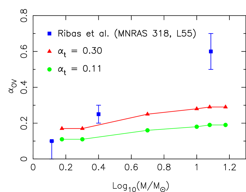
With this modified length scale, we repeat the comparison between MLT and KCT for two cases, one with $\alpha_{\mathrm{t}}=0.11$ and the other with $\alpha_{\mathrm{t}}=0.30$ both values in accord with stellar evolution of Procyon A (see Section 3.3). We determine the amount of overshoot – measured in pressure scale heights – needed to reproduce the models employing KCT. As can be seen in Figure 1 our models show less overshoot compared to Kuhfuß’s original analysis: with $\alpha_{\mathrm{t}}=0.3$ we find $\alpha_{\mathrm{OV}}=0.17$ for a $1.5\,{M}_{\sun}$ star and $\alpha_{\mathrm{OV}}=0.29$ for a $15\,{M}_{\sun}$ star. Since Ribas et al. (2000) claim an increase of core overshoot for increasing mass by measurements of eclipsing binaries we also ask whether KCT can naturally explain this behavior. Indeed, we can see a moderate increase of overshoot with mass. Nonetheless, the increase is not pronounced enough to explain the large overshoot of $0.6$ claimed for the $11.1\,{M}_{\sun}$ star V380 Cyg. By increasing the mixing length parameter $\alpha_{\mathrm{MLT}}$ the increase of overshoot with mass can be enhanced slightly but an overshoot of $0.6$ remains out of reach.

It is obvious to think rotation could play an important role in increasing the core through rotational mixing in a star of such high mass. Guinan et al. (2000) have carried out a detailed analysis of this system reaching the conclusion that the slow rotation of this star cannot account for substantial additional core size increase. The recently derived overshoot of $\alpha_{\mathrm{OV}}=0.10\pm 0.05$ for another high mass star with $9\,{M}_{\sun}$ (Aerts et al. 2003; Dupret et al. 2004) seems to indicate that the large overshoot for V380 Cyg may not be a universal property of high mass stars.

3 Stellar Models of Procyon A

3.1 Constraints from Observations

Procyon A and its companion white dwarf constitute a visual binary system with a 40 yr period. The redetermined mass of Procyon A based on 250 photographic plates of observations between 1912 and 1995 combined with modern direct measurements of the angular separation of the pair utilizing HST Planetary Camera and ground based coronagraph data are given by Girard et al. (2000) with a derived mass of $1.497\pm 0.037\,{M}_{\sun}$. The same study also determines the parallax of Procyon A to be $0\farcs 2832\pm 0\farcs 0015$ a value different from the Hipparcos result $p=0\farcs 28593\pm 0\farcs 00088$. We take the mean value of both independent measurements and adopt the difference to the upper and lower bound of these measurements as our $1\sigma$ error estimate thereby yielding $p=0\farcs 28457\pm 0\farcs 0025$. The larger adopted uncertainties for the parallax lead to larger error bars for Procyon A’s radius and luminosity than otherwise expected if we had used the quoted errors from the actual measurements.

The radius of Procyon A can be retrieved using the stellar angular diameter data derived from optical interferometry $\theta=(5\farcs 51\pm 0\farcs 05)\times 10^{-3}$ (Mozurkewich et al. 1991). Taking the center-to-limb variation from detailed model atmospheres into account Allende Prieto et al. (2002) correct this value slightly: $\theta=(5\farcs 48\pm 0\farcs 05)\times 10^{-3}$. When combined with parallax of $p=0\farcs 28457\pm 0\farcs 0025$ and applying the laws of error propagation to the three quantities involved one finds the radius

$$R\simeq\frac{\theta}{2p\,\tan(\theta_{\sun}/2)}=2.070\pm 0.026\,{R}_{\sun}$$ (15)

adopting $\theta_{\sun}/2=959\farcs 64\pm 0\farcs 02$ (Chollet & Sinceac 1999). This result is statistically identical to the independent angular diameter measurement of Kervella et al. (2004).

The effective temperature is measured with the averaged bolometric flux (Fuhrmann et al. 1997) $F_{\mathrm{BOL}}=(18.20\pm 0.43)\times 10^{-6}\,\,\mbox{erg}\,\mbox{cm}^{-2}\,\mbox{s}^{-1}$:

$$T_{\mathrm{eff}}=7400\times\left(\frac{F_{\mathrm{BOL}}}{\theta^{2}}\right)^{\!\!{1/4}}=6530\pm 50\,\mbox{K}$$ (16)

With an absolute distance of Procyon A from earth given by the parallax measurement, $d=3.0857\times 10^{18}\,\mbox{cm}/p(\arcsec)$ we derive the intrinsic luminosity (${L}_{\sun}=3.833\times 10^{33}\,\,\mbox{erg}\,\mbox{s}^{-1}$)

$$L=4\pi d^{2}F_{\mathrm{BOL}}=(7.016\pm 0.21)\,{L}_{\sun}$$ (17)

and we use the value $\log_{10}(L/{L}_{\sun})=0.8461\pm 0.013$ throughout this study.

3.2 Constructing Tracks consistent with Observations

Since parallax $p$, angular diameter $\theta$ and bolometric flux $F_{\mathrm{BOL}}$ are measured with completely independent techniques and data sets the derived basic stellar parameters luminosity $L$, radius $R$ and effective temperature $T_{\mathrm{eff}}$ can be jointly used to constrain stellar models for Procyon A . Therefore we require all stellar models for Procyon A to fall into a three dimensional error box given by observational constraints for $L$, $R$ and $T_{\mathrm{eff}}$. With help of the identity $L=4\pi R^{2}\sigma T_{\mathrm{eff}}^{4}$ one of the constraints can be projected onto a plane given by the remaining two. If we look, for example, at the $R$-$L$-plane the error box is given by a hexagonal shape. Both $1\sigma$ and $2\sigma$ limits as inferred from Section 3.1 are shown (Figure 2).

Our model calculations start from the ZAMS with the default parameters of mass $M=1.497\,{M}_{\sun}$, solar hydrogen content $X=0.70$, solar metallicity $Z=0.018$, mixing length $\alpha_{\mathrm{MLT}}=1.7$, no overshoot and no envelope element diffusion. We now vary the mass $M=\{1.423$, $1.435$, $1.45$, $[1.46$, $1.47$, $1.48$, $1.485$, $1.49$, $1.497$, $1.509$, $1.515$, $1.52$, $1.53$, $1.534]$, $1.55$, $1.56$, $1.571\}$, hydrogen content $X=\{0.68$, $[0.69$, $0.70$, $0.71]$, $0.72\}$, metallicity $Z=\{0.016$, $[0.017$, $0.018$, $0.019]$, $0.020\}$, mixing length parameter $\{[1.5$, $1.6$, $1.7]\}$ and convection description $CT=\{[1$, $2$, $3]\}$ with the associated overshoot parameters $\alpha_{\mathrm{OM}}=\{[0.0$, $0.2$, $0.4$, $0.6$, $0.8]\}$, $\alpha_{\mathrm{OV}}=\{[0.2$, $0.4$, $0.6]\}$ and $\alpha_{\mathrm{t}}=\{[0.2$, $0.6$, $3.0]\}$. The full set of all combinations required us to calculate $14025$ different models. Of these, $2938$ fell in the observational $2\sigma$ error box and $1541$ in the $1\sigma$ error box. In order to explore the sensitivity of our results to uncertainties in the input parameters, we also study a more restricted parameter set given by all combinations within the values of the innermost brackets. The restricted set consists of $3564$ models, of which $712$ qualify within the $2\sigma$ and $354$ in the $1\sigma$ observational limits. Models with overshoot are calculated in the case of three different overshoot prescriptions CT1-CT3 by varying the overshoot parameter relevant to the adopted theory.

For each stellar track that falls within the error box we pick out five models, two at the inner and outer $2\sigma$ boundaries, two at the inner and outer $1\sigma$ boundaries and finally one close to the center of the error box. In instances in which models do not cross the $1\sigma$ box only two models are picked out. On all picked out models, a full pulsational analysis is performed and discussed in Section 4.

All models within the $1\sigma$ error box are found to be in the main sequence phase of evolution. Chaboyer, Demarque, & Guenther (1999) also consider a model in the hydrogen shell burning subgiant phase. If we allow the full $2\sigma$ we also cannot exclude shell burning phase models from stellar tracks. However, subgiant models are only found for initial masses of $M\leq 1.47\,{M}_{\sun}$. It is worth noting, that with overshoot, it becomes increasingly harder to bring a shell burning model in accord with the observational ($2\sigma$) constraints. By calculating two additional sets of models with $\alpha_{\mathrm{OM}}=0.02$ and $\alpha_{\mathrm{OM}}=0.05$ and carefully taking into account all possible combinations within the remaining parameters we could verify that tiny amounts of overshoot of $\alpha_{\mathrm{OM}}>0.05$ completely inhibit the shell burning model as a viable possibility.

3.3 Constraints on Core Overshoot

As can be seen in Figure 2 models with no overshoot are consistent with the observational constraints. At present, we cannot claim evidence for or rule out overshoot on the basis of traditional stellar modeling. But we can try to provide upper limits and best fit values on overshoot for the different overshoot prescriptions.

Since the stellar luminosity is — to first order — a function of mass, a lower mass value for Procyon A enforces more overshoot in an effort to increase the model luminosity to the observed value. Overshoot generally causes larger convective cores, thereby transforming more hydrogen into helium which in the course of nuclear burning leads to a higher mass averaged molecular weight $\bar{\mu}$. Being also proportional to $\bar{\mu}^{4}$ the luminosity is sensitively increased by small amounts of overshoot.

Best fit values are ascertained by adopting default stellar parameters and adding overshoot until the tracks coincide with the best fit locus defined halfway between the radius and halfway between the luminosity uncertainties, the latter taken at the best fit radius. The best fit values are $\alpha_{\mathrm{OM}}=0.06$, $\alpha_{\mathrm{OV}}=0.06$ and $\alpha_{\mathrm{t}}=0.03$ (Figure 3).

Smaller mass and $\alpha_{\mathrm{MLT}}$ and larger $X$, $Z$ shift tracks to lower luminosities thereby requiring more overshoot in order to bring the tracks back into the observational error box. We now simultaneously alter all four input parameters such that maximal overshoot is needed.

The first set of upper overshoot limits is derived by using a mass of $M=1.46\,{M}_{\sun}$, $\alpha_{\mathrm{MLT}}=1.6$ and hydrogen $X=0.71$ and metallicity of $Z=0.019$. These input parameters correspond to the set of restricted limits Section 3.2. We denote the limits by this procedure weak limits and they are $\alpha_{\mathrm{OM}}\leq 0.65$, $\alpha_{\mathrm{OV}}\leq 0.75$. (see Figure 4).

The second set of upper limits, the strong limits, are found by repeating this procedure for the minimally allowed observational mass of $M=1.423\,{M}_{\sun}$, $\alpha_{\mathrm{MLT}}=1.6$ and the highest values allowed for in this study for hydrogen and the metallicity, i.e., $X=0.72$ and $Z=0.020$. Thus we take the most extreme values in favor of overshoot. The strong limits are $\alpha_{\mathrm{OM}}\leq 1.18$ and $\alpha_{\mathrm{OV}}\leq 1.13$ (see Figure 5).

An interesting property of the Kuhfuß (1986)-theory is, that the core size cannot be increased above a certain limit regardless of the overshoot parameter $\alpha_{\mathrm{t}}$. For Procyon, the extent of the overshoot region is not substantially increased above $\alpha_{\mathrm{t}}=5$. This behavior is rooted in the KCT and we will discuss this in more detail in the next section (Section 3.4).

3.4 Extent of Overshoot region with KCT

It is important to point out that the role of the free parameter $\alpha_{\mathrm{t}}$ is different compared to the free parameters $\alpha_{\mathrm{OM}}$ or $\alpha_{\mathrm{OV}}$. Increasing the latter two will always lead to more extended convective cores — up until the star is fully convective. On the other hand, $\alpha_{\mathrm{t}}$ is a factor regulating the relative importance of the non-local terms, i.e., the third term in equation  8. Increasing the non-local coupling does not always lead to more extended overshoot. In fact, extremely large values for $\alpha_{\mathrm{OV}}$ lead to smaller overshoot extents.

The run of the non-local term is shown in Figure  6 (left panel) for three different and extremely high values for $\alpha_{\mathrm{t}}$. The largest convective cores can be attained with $\alpha_{\mathrm{t}}\sim 100$ which corresponds to an overshoot distance of $\sim 0.4\,H_{\!{P}}$. The model with $\alpha_{\mathrm{t}}=1000$ produces smaller overshoot regions. The reason for this lies in the run of the non-local term itself: above the Schwarzschild boundary this term is positive and acts towards more extended cores but in the inner regions it is negative and acts to decrease the overshoot distance. The net effect can be studied in Figure  6 (right panel) where we show the corresponding stationary solution of the turbulent kinetic energy. High values of $\alpha_{\mathrm{t}}$ finally decrease the turbulent kinetic energy in the inner part and thereby the velocity of the eddies at the Schwarzschild boundary such that they lack the energy to travel far.

In both panels of Figure  6 we show how the maximum core size derived from the Kuhfuß theory compares with the well known integral criterion derived by Roxburgh (1978). As can be seen from the figures, the maximally allowed sizes by KCT almost exactly match the core size predicted by the integral criterion.

With this property of the more physically motivated overshoot prescription it would be possible to constrain the uncertainties of mass, hydrogen content, metallicity and mixing-length parameter. Since the scope of this paper is to find observational constraints from traditional stellar modeling when combined with seismological data we do not explore this possibility in more detail. However, when comparing the different overshoot prescriptions in the next sections we must keep in mind that models of Procyon A employing the Kuhfuß-theory inherit convective cores with an overshoot distance not larger than $\sim 0.4\,H_{\!{P}}$.

4 Pulsation Analysis of Procyon A

4.1 p-modes

Ground based attempts to measure the p-mode large spacings have so far been inconclusive (Brown et al. 1991; Bedford et al. 1995; Mosser et al. 1998; Barban et al. 1999; Martić et al. 1999). Of these works Mosser et al. (1998) derive a tentative value for the large spacing of $53\,\mu\mbox{Hz}$. Barban et al. (1999) and Martić et al. (1999) claim to have observed excess power and spacings of $55\,\mu\mbox{Hz}$ which would be compatible with the theoretical predictions (see Figure 7). However, all these measurements have been restricted to single site measurements producing data contaminated by significant amplitudes of daily aliases.

While p-mode frequencies as a function of radial and azimuthal order $\nu(n,l)$ hold the most accurate and detailed information about the run of sound speed within a star, one cannot hope to match the model to all frequencies by blindly searching the allowed parameter space. This procedure would only work if a stellar model matched the star as well as our solar models match the Sun. Also, inversion techniques cannot be easily applied to stars because we are only able to observe low azimuthal order p-modes, hence, cannot construct detailed enough kernels to unambiguously span the surface layers. Nonetheless, we can make use of averaged quantities which dispense some of the rich information contained in the oscillation spectrum but still pose additional and useful constraints on the stellar model. Such information is available from the averaged first- and second-order frequency spacings (cf., Christensen-Dalsgaard 1984, p. 11).

The frequency spacings for Procyon A have been calculated and analyzed extensively before (Guenther & Demarque 1993; Chaboyer et al. 1999). They noted that mode bumping occurs in Procyon A and that the irregular spacing associated with mode bumping could be used to pin down Procyon’s evolutionary phase. Independent of the oscillation data, they also noted an inconsistency between the astrometric mass of Procyon and the mass obtained from fitting their models to Procyon’s position in the HRD, with the latter turning out to be correct (Girard et al. 2000).

In this paper we discuss what existing observational data can tell us about convective core overshoot, and we ask how future observational data, including seismic data, can help constrain the models further.

For all our models that fall within the error box we calculate the $l=0,1,2,3$ p-modes from radial order $n=0$ up to about $35$ using the non-radial pulsation code JIG developed by Guenther (1994). Mode bumping for Procyon A occurs at low radial orders between $\sim 0$ – $16$. Mode bumping, also referred to as avoided crossings, occurs in more evolved stars when the molecular weight gradient left behind by nuclear burning leaves a barrier that traps g-modes in the core. When the frequencies of the g-modes increase, as the star evolves, they eventually cross through the frequencies of the lowest radial order p-modes. In regions of frequency overlap the modes mix, perturbing the frequencies. Therefore, mixed modes contain extremely interesting information on core overshoot. Since we are dealing with a resonance phenomenon very accurate stellar models are required. One of us (D.B.G) is exploring these possibilities in a subsequent paper.

The p-modes with radial order greater than about $16$ show regular spacings in all our models. It is this information that is likely the first to be detected and measured accurately.

4.1.1 Large Spacings

The first order frequency spacings or large spacings are defined as

$$\Delta\nu(n,l)=\nu(n,l)-\nu(n-1,l)\,\,\mbox{.}$$ (18)

It follows from Tassoul (1980) asymptotic theory that high radial order modes are approximately equally spaced with

$$\Delta\nu\simeq\left(2\int_{0}^{R}\frac{dr}{c}\right)^{-1}$$ (19)

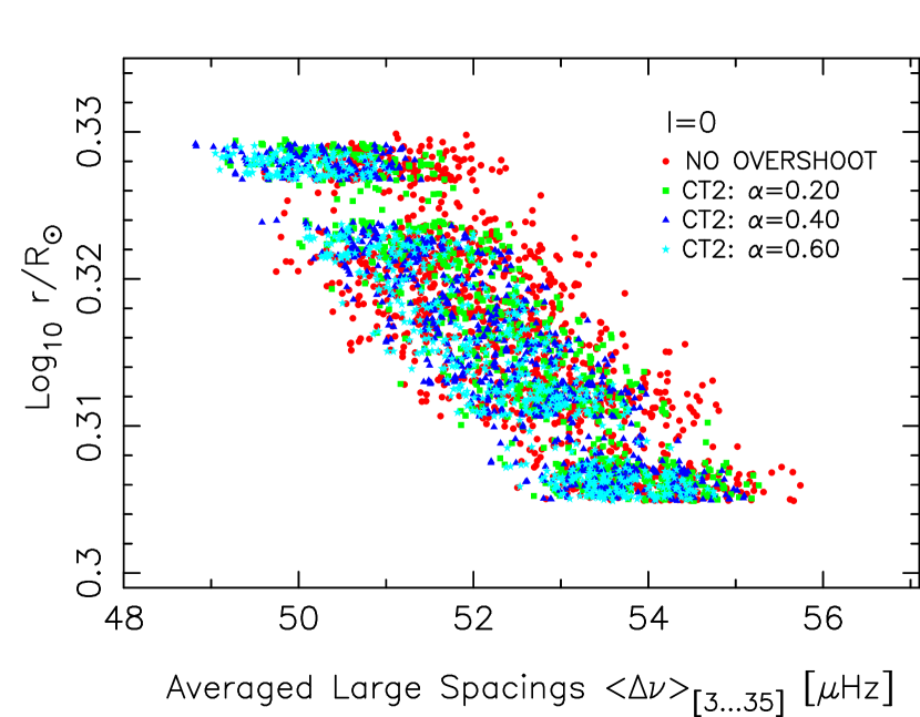
where $R$ is the radius and $c$ is the sound speed. Since the integrand is proportional to the inverse of the sound speed the large spacings are most sensitive to the outer layers of the star where $c$ is smallest. The spacings depend on the radius and the mass of the star with $\delta\nu/\nu\propto\delta r/R_{*}-\delta M/(3M_{*})$. Can we improve on Procyon A’s radius estimate by making use of the information provided by the large spacings? Indeed we can, as seen in Figure 7. Here we plot the large spacings averaged over the range $n=[3\ldots 35]$ versus stellar radius for the order $l=0$. Each point in the diagram corresponds to a calculated stellar model with $CT2$. The spread from a straight line shows the full set of model uncertainties due to different mass, overshoot, metallicity and mixing length parameters. We verified that models corresponding to the other convection prescriptions, i.e., from $CT1$ and $CT3$ do not widen the spread. The spread is tight enough to improve on the radius by a factor of two for measured averaged large spacings $\lesssim 51\,\mu\mbox{Hz}$ and $\gtrsim 54\,\mu\mbox{Hz}$. The radius measurement in the range $51$-$54\,\mu\mbox{Hz}$ can be improved upon only with smaller improvement factors and it is impossible to do so in the range $52$-$52.5\,\mu\mbox{Hz}$. The $l=1,2$ modes could provide additional independent measurements but it turns out that there is more than one region where models cluster which leads to a wider spread.

Since the large spacings are sensitive to the outer layers we do not expect them to be sensitive to different core overshoot. For different orders of $l$ we looked at the convective core size as a function of the averaged large spacings. The points scatter all over the diagram so no correlation between the large spacings and the convective core size exists. This fact is indeed fortunate if we want to use the large spacings for an independent measure of the stellar radius.

4.1.2 Small Spacings

The small spacings are defined by

$$\delta\nu(n,l)=\nu(n,l)-\nu(n-1,l+2)\,\,\mbox{.}$$ (20)

Again, asymptotic approximations predict equal spacings proportional to an integral with an integrand of $r^{-1}(dc/dr)$ which increases with depth. Thus, the small spacings are most sensitive to the interior where the integrand is largest.

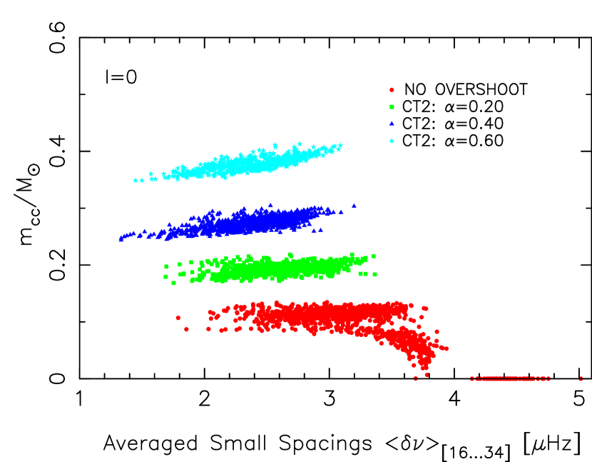
Therefore, we want to know whether the small spacings could be used to discriminate between different convective core sizes. We show the small spacings versus the core size, averaged over radial orders $n=[16\ldots 34]$. If we look at the $l=0$, $CT2$ models in Figure 8 we see that for frequency spacings $>3.4\,\mu\mbox{Hz}$ only models without overshoot can be found. In addition, almost all subgiant models which can be identified as the ones exhibiting zero convective core sizes occupy exclusively the region $>4\,\mu\mbox{Hz}$. This result is robust, because it does not depend on the overshoot prescriptions since only tiny amounts of overshoot inhibit the subgiant models completely. Thus, the averaged small spacings for $l=0$ might provide the necessary measurement needed to discriminate between the two evolutionary stages.

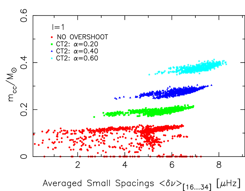
In comparison to the $l=0$ modes the $l=1$ frequency spacings are more influenced by the different amounts of overshoot. Here, overshoot leads to larger frequency spacings (Figure 9). Due to the spreads in parameter space, inferring the overshoot parameter or convective core size is difficult: If, for example, a frequency spacing of $5\,\mu\mbox{Hz}$ is measured, $\alpha_{\mathrm{OV}}$ could be anywhere between zero and $0.6$. The situation is more favorable for a measured frequency spacing of $8\,\mu\mbox{Hz}$ where one could infer an $\alpha_{\mathrm{OV}}\sim 0.4\pm 0.2$. As will be shown in the next section, the g-modes are better suited to yield a core size measurement.

4.2 g-modes

Although g-modes have never been detected conclusively in the Sun (Appourchaux et al. 2000; Wachter et al. 2003), it may be possible to detect them in Procyon A. The convection zone in the sun’s atmosphere constitutes a long attenuating tunnel for g-modes (Stix 2002, p.234) in strong contrast to Procyon’s very thin convective envelope of $\sim 10^{-5}\,{M}_{*}$. On this basis we hope that for existing and planned asteroseismic observations, some effort is made to detect g-modes in Procyon A .

4.2.1 Period Spacings

For all our models that fall within the error box we calculate the $l=1,2,3$ g-modes from radial order $n=-2$ to about $-30(l=1)$, $-70(l=2)$, $-80(l=3)$ respectively with the non-radial pulsation code JIG. In the following, we use the full set of combinations, i.e., full input parameter space and $2\sigma$ observational error box. As described in Section 3.2 we perform a pulsational analysis on five selected models within the error box, if possible. For one selected model, we show their periods as a function of radial order $n$ (Figures 10). There are a few gaps in the range of g-modes computed, an artifact of the automated search technique used by the pulsation program. This is of no consequence here since we are here only interested in computing the slope of the curves. We use a least-square algorithm to fit linear functions to the calculated gravity modes. The steepness of these lines gives the period spacings which can be explained by asymptotic theory (Section 4.2.2). Since asymptotic theory predicts a unique period spacing any scatter of calculated frequencies from a straight line indicates deviations from this theory. There is some scatter at very low $n$ where asymptotic theory does not hold and also where mode bumping is likely to occur. In addition, as can be seen in Figure 10 but is present in all calculated g-mode spectra, the scatter is larger for lower $l$ degree modes especially at high radial order. This scatter may well contain information about stellar structure beyond the information contained in the period spacing but we confine ourselves to the latter because the scatter is a quantity much more difficult to measure.

4.2.2 Asymptotic Theory

According to the asymptotic theory (Tassoul 1980), the period $\Pi_{nl}$ of low degree $l$ and high radial order $n$ ($n\gg l\simeq 1$) is, to first order, given by (Unno et al. 1989, p.83)

$$\Pi_{nl}\simeq\frac{(n+l/2-1/4)}{\sqrt{l(l+1)}}\,\Pi_{0}$$ (21)

with

$$\Pi_{0}=2\pi^{2}\left[\int_{\ln(r_{\mathrm{cz}})}^{\ln(r_{\mathrm{b}})}N(r)\,d\ln r\right]^{-1}$$ (22)

where $r_{\mathrm{cz}}$ is the radius of the core convection zone, $r_{\mathrm{b}}$ the radius at the bottom of the convective envelope and $N$ is the Brunt-Väisälä frequency. This formula establishes a regular period spacing $\Pi_{l}$ which is given by

$$\Pi_{l}=\frac{2\pi^{2}}{\sqrt{l(l+1)}}\left[\int_{\ln(r_{\mathrm{cz}})}^{\ln(r_{\mathrm{b}})}N(r)\,d\ln r\right]^{-1}$$ (23)

As can be seen by this formula, the higher degree $l$ modes do not hold additional information about the star’s structure. The most important contributions to the integral in equation (23) come from the fully ionized inner regions of the star, hence the square of the Brunt-Väisälä frequency, $N^{2}$, is well approximated by making use of the gradient of the mean molecular weight, $\mu$, i.e.,

$$N^{2}=\frac{g^{2}\rho}{P}\left[\frac{4-3\beta}{\beta}(\nabla_{\!\mathrm{ad}}-\nabla)+\varphi\nabla_{\!{\mu}}\right]$$ (24)

where we denote local gravitational acceleration $g=(Gm)/r^{2}$, density $\rho$, pressure $P$, ratio of gas to total pressure $\beta=P_{\mathrm{gas}}/P$, adiabatic gradient $\nabla_{\!\mathrm{ad}}$ and actual stellar temperature gradient $\nabla$. The Brunt-Väisälä frequency gives the frequency by which a bubble of gas oscillates vertically around its equilibrium position under gravity. The frequency is therefore proportional to its restoring buoyancy force which is given by the spatial entropy gradient, or alternatively, by $\nabla_{\!\mathrm{ad}}-\nabla$. Another contribution to the Brunt-Väisälä frequency is given by the second term in brackets of equation (24): The molecular weight gradient which can increase or decrease the frequency depending on the sign of $\nabla_{\!{\mu}}$.

4.2.3 g-mode Characteristics in Procyon A

In the case of the late main-sequence star Procyon A the Brunt-Väisälä frequency is largest in parts of varying molecular weight gradient which is left over from the receding core convection zone of main hydrogen burning (Figure 11 ). The molecular weight gradient for mass shells greater than about $0.4\,{M}_{*}$ remain untouched and the buoyancy starts to dominate equation (24). Although buoyancy constantly increases toward the outer stellar layers the drop-off of density reduces its contributions to the frequency exhibiting a maximum around $0.6\,{M}_{*}$. These general characteristics are true for all our models irrespective of any overshoot, because this basic structure can be found in all late main-sequence stars that have convective cores.

4.2.4 What g-modes reveal about overshoot

With asymptotic theory (Section 4.2.2), we can gain further insight on how overshoot influences the g-mode period spacings. In order to show the differences in the Brunt-Väisälä frequency inscribed by different amounts of overshoot we show Figure 12 where we compare KCT overshoot for two different overshoot parameters $\alpha_{\mathrm{t}}=0.17$ and $\alpha_{\mathrm{t}}=0.30$. We recall, that since overshoot increases the size of the convective region it taps a larger hydrogen fuel reservoir. Models which fall into the same error box and exhibit larger overshoot have not used up hydrogen as much and therefore the molecular weight gradient is shallower albeit increasing the period spacing $\Pi_{0}$. Not so obvious at first glance but even more important is the inner cutoff radius $r_{\mathrm{cz}}$ which is larger for models with overshoot, reduces the Brunt-Väisälä frequency and therefore also increases the period spacing $\Pi_{0}$.

These effects on the period spacings imply, that for given and fixed overshoot prescription and input parameters (mass, metallicity, etc.) a one-to-one relation between period spacings and convective core size could be made. On the other hand, the situation here is more complicated since we must take a range of uncertainties into account.

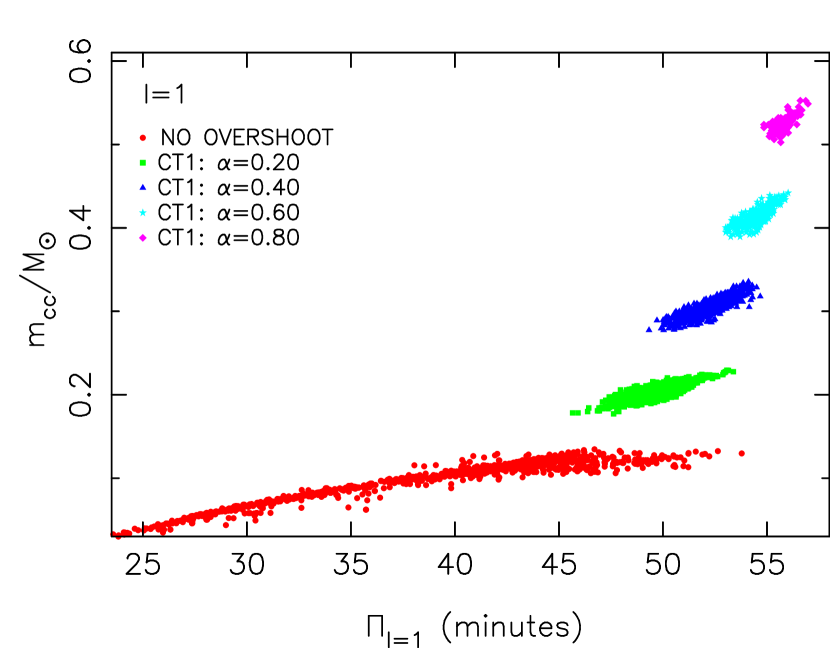
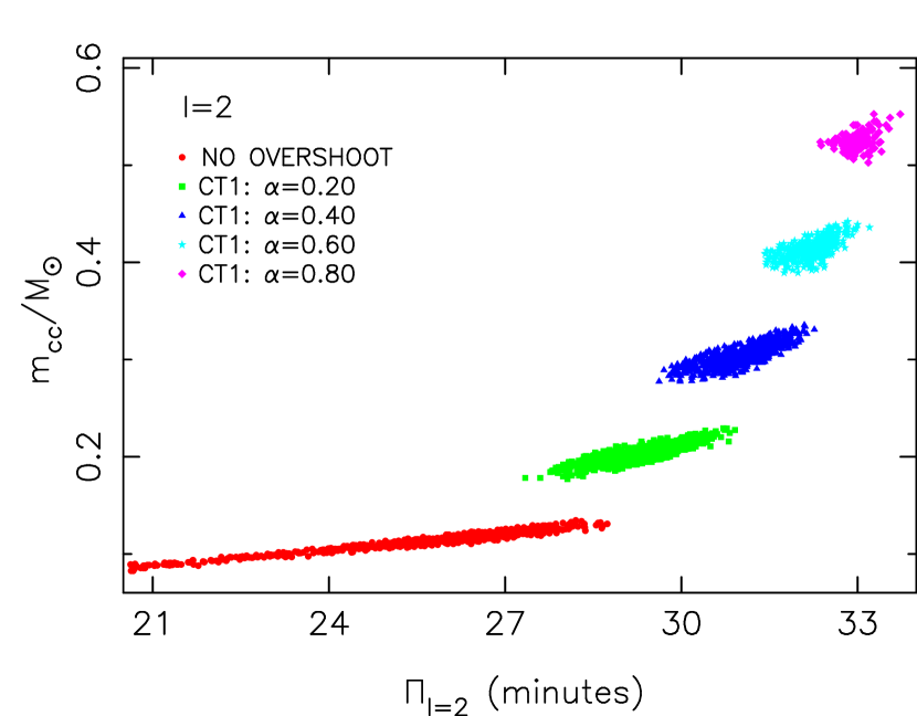
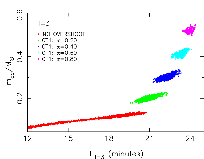
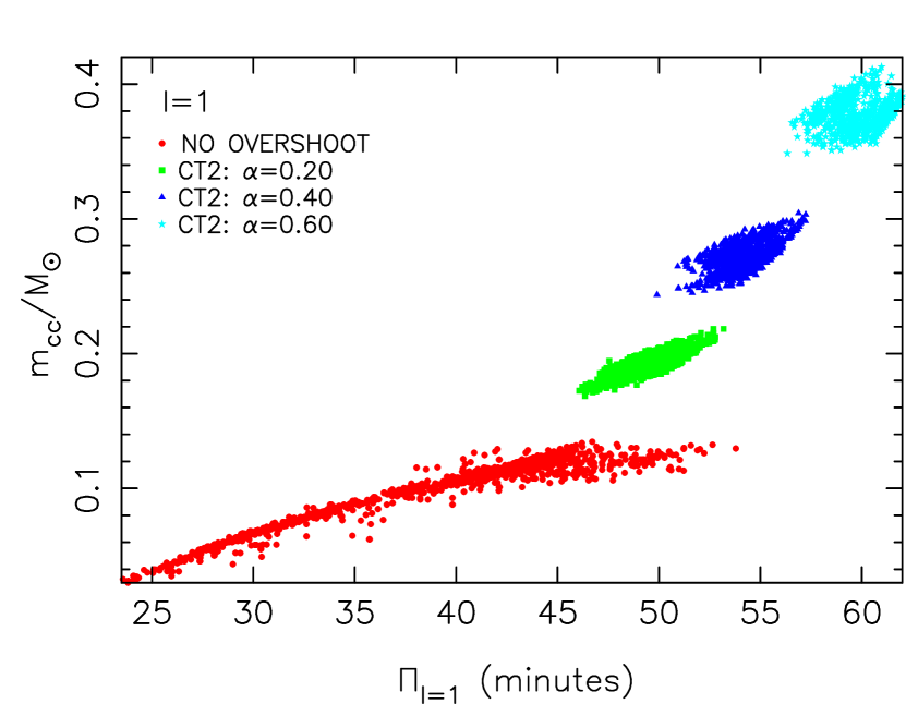
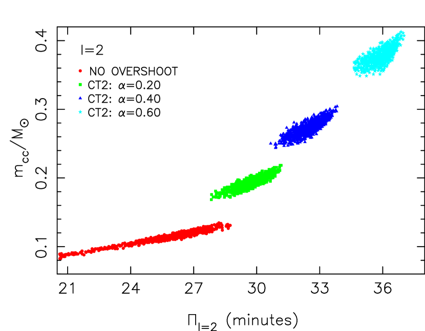
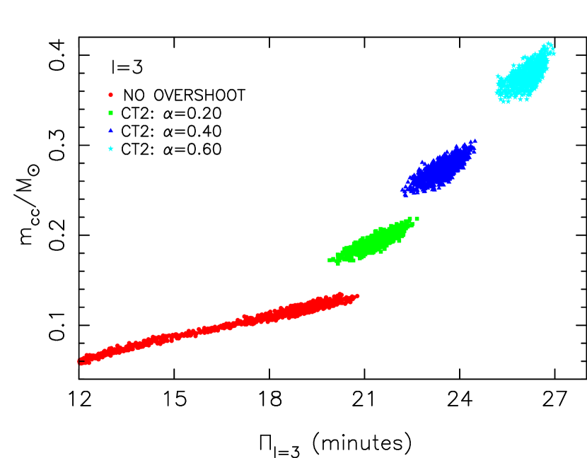
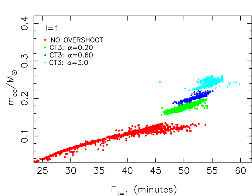
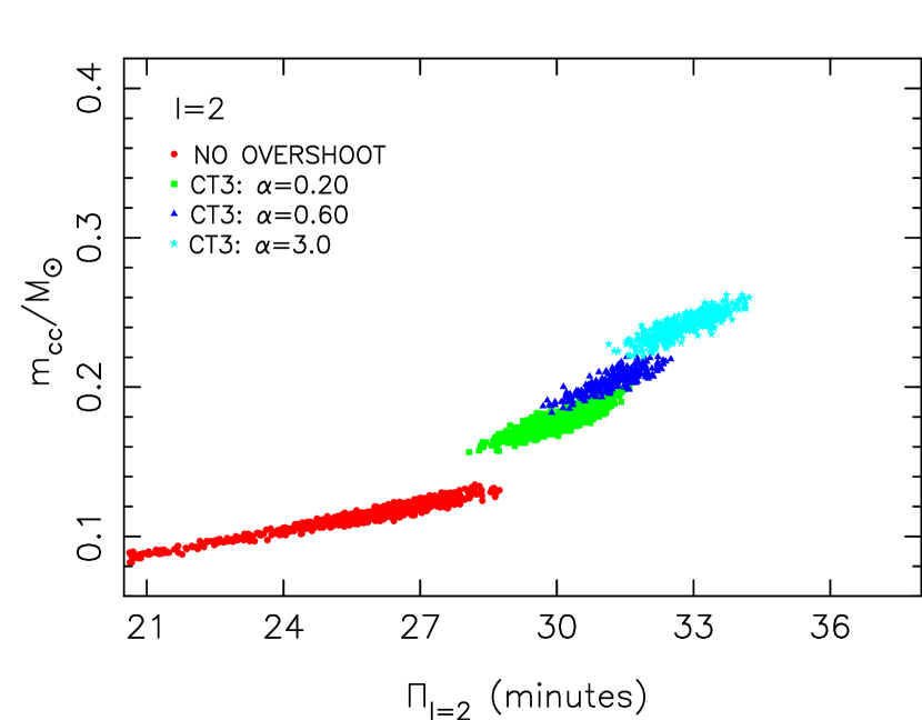
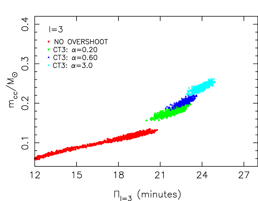
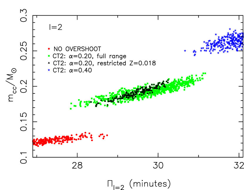
Here we present the relation between period spacings and convective core size in Figures 13-21 for all models of the full input parameter set that fall in the $2\sigma$ observational error box. We can see a strong albeit not perfect correlation of the period spacing with convective core size. This can be used to measure the overshoot parameter within a given overshoot prescription provided it is possible to derive the period spacing from observational data. However, within the current uncertainties, this measurement is not extremely accurate. For adopted overshoot prescription and given value of the period spacings the derived overshoot parameter can be determined with an accuracy of $\pm 0.15\,H_{\!{P}}$ (CT1), $\pm 0.10\,H_{\!{P}}$ (CT2) and $\pm 0.05\,H_{\!{P}}$ (CT3). Note that although the overshoot parameter $\alpha_{\mathrm{t}}$ can only be constrained within $\pm 1.4$ the overshoot extend measured in pressure scale heights is most favorably constrained with CT3. We will see in the next Section 4.3 what uncertainties need to be improved upon in order to be able to get a more constrained overshoot estimate.

Still, we can deduct valuable information about the convective core size, especially in certain period regions. Whereas models without overshoot occupy the regions with period spacings of $25-45(l=1)$, $21-27(l=2)$ and $12-19(l=3)$ minutes the models with overshoot have generally longer period spacings. Thus we find, that irrespective of the different overshoot prescriptions, there exists a period regime for models without overshoot that is cleanly separated from the overshoot cases.

For period spacings greater than $45(l=1)$, $27(l=2)$ and $19(l=3)$ we get two different types of overlaps. First, for given adopted overshoot prescription and overshoot parameter, there is a spread due to the input model and observational uncertainties. As seen in Figures 13-21 these spreads constitute islands which correspond to a period regime which overlaps with neighboring ones. The less overlap the more accurate it is possible to determine the overshoot parameter from the period spacings. Note that the overlap is stronger for the CT1 models when compared to the CT2 ones. The second overlap stems from the fact that we do not know the correct overshoot theory before hand. For example, if we look at the $l=2$ plots (Figures 14,17) at a period of 31 minutes with CT1 we get $\alpha_{\mathrm{OM}}=0.35\pm 0.15$, on the other hand, with CT2 we determine $\alpha_{\mathrm{OV}}=0.3\pm 0.10$.

Both types of overlaps could be reduced. The first one could be reduced by better observational data that is able to narrow down the error box and the set of input parameters. The most crucial observational parameters for this will be identified in the next Section 4.3. The second type of overlaps that result from the different overshoot prescriptions is even harder to overcome: when the outlined analysis presented here for Procyon A is applied to many different, at least equally good constrained stars, it might be possible to do so in the future.

4.3 Sensitivity of Results

In the last section we demonstrated that, for a given convection prescription, uncertainties on our models imposed by both the observational error box and the possible initial input parameter space lead to overlaps in the period spacings thereby imposing uncertainties on future measurements of the overshoot parameter. For upcoming observations on Procyon A it might be enlightening which parameters need to be constrained the most in order to be able to determine the overshoot parameter with more accuracy.

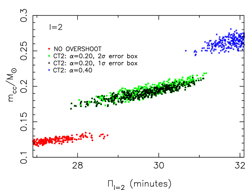
First we want to determine the effects of narrowing the observational error box. To do so, we only allow those models to qualify as viable models that fall into the $1\sigma$ observational error box. As seen in Figure 22 the period spread occupied by the $CT2$, $l=2$, $\alpha_{\mathrm{OV}}=0.2$ $1\sigma$ error box models (triangles) is not smaller compared to the full model set (squares). Thus, narrowing the error box to $1\sigma$ does not help in improving the accuracy of the overshoot parameter.

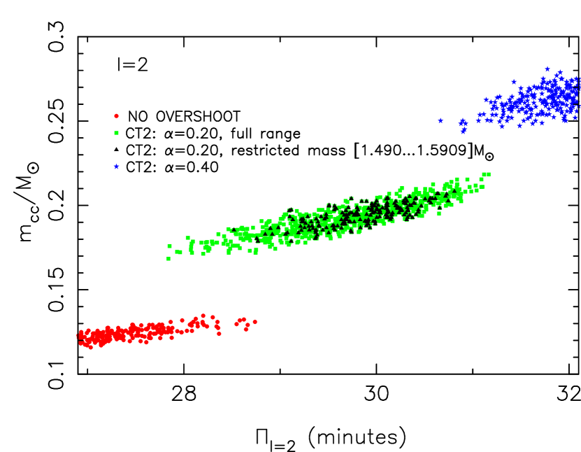
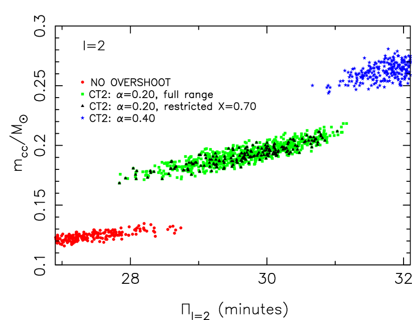
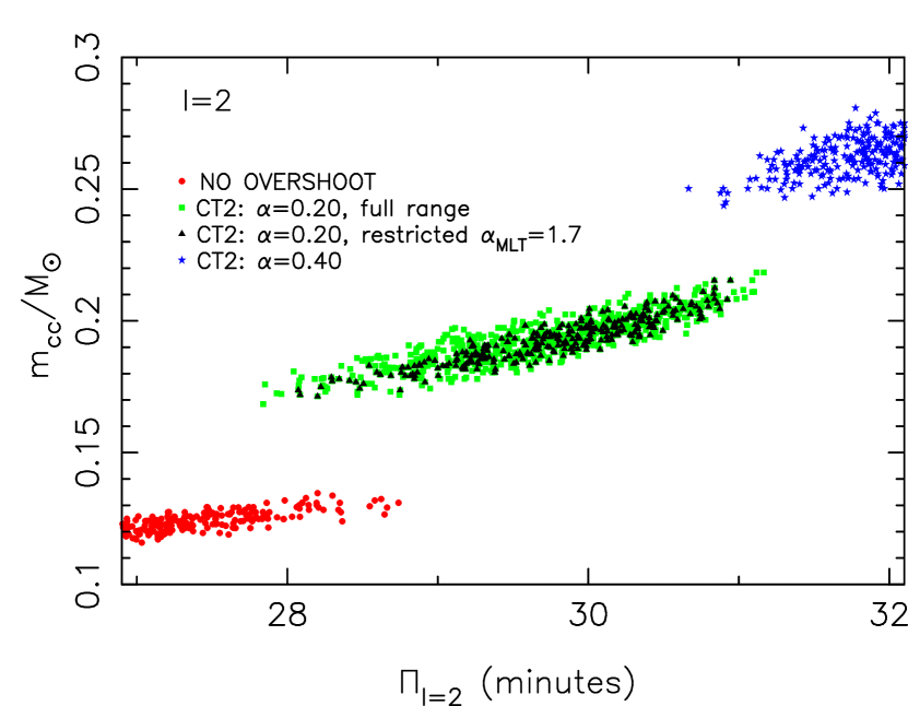
Next we assess the possible benefits arising from constraining one out of the five input parameters, i.e., mass (Figure 23), hydrogen fraction (Figure 24), metallicity (Figure 25) and mixing length parameter (Figure 26). As can be seen in the Figures the most crucial input parameters turn out to be both the mass and the metallicity. Measuring those two more precisely can bring down the spread by a factor of three.

5 Summary and Conclusions

We have constructed a comprehensive set of stellar models for Procyon A with varying model assumptions on mass, hydrogen content, metallicity, mixing length parameter, adopted core overshoot prescription and overshoot parameters in an effort to single out current and promising future observables that constrain the amount and possibly the nature of core overshoot in stellar interiors.

In this study, effects of rotation have not been taken into account. Procyon A is a slow rotator with a measured rotational velocity of $v\sin i=3.2\,\mbox{km}\,\mbox{s}^{-1}$. Rotation is therefore expected to produce multiplets for higher azimuthal modes than the fundamental with splittings on the order of $0.5\,\mu\mbox{Hz}$. This has to be kept in mind when comparing the predictions made here with actual observations.

The classical treatment of overshoot in stars — extending the core size by some fraction of the pressure scale height — is merely a measure of overshoot and cannot be regarded as an accurate description of the underlying physics. For this basic reason we implement a physically better motivated non-local convection theory developed by Kuhfuß (1986). We neglect a number of terms present in this theory, foremost its time-dependency and some others expected to be only important in evolutionary phases that must be followed on a dynamical timescale. More relevant to this study is the choice of the five free parameters present in the theory. Reasonable choices on four can be made in analogy with MLT and we only vary one parameter, $\alpha_{\mathrm{t}}$, which is the most relevant to the amount of overshoot. However, we stress that all parameters must be eventually calibrated, a task that might prove possible in the future if the methods presented in this paper are applied to many stars alike. Regardless of the actual adopted numbers, we do find a moderate increase of the amount of core overshoot with increasing stellar mass up to about $15\,{M}_{\sun}$. In comparison with Kuhfuß’s original analysis we find smaller amounts of overshoot for the same adopted parameters mainly because we limit the pressure scale height in the stellar center. We are not certain, whether the implementation by Kuhfuß (1987) omitted the molecular weight gradient which would constitute an additional reason why he found overall larger convective core sizes.

We also show, that models calculated with the Kuhfuß convection theory contain convective core overshoot extents smaller than $\sim 0.4\,H_{\!{P}}$ regardless of the overshoot parameter $\alpha_{\mathrm{t}}$ adopted. This behavior is rooted in the non-local treatment of the theory: Since overshooting eddies transport internal energy farther out it also lowers the internal energy in deeper regions of the core. But the deep regions provide the driving necessary for overshoot to occur. Thus we have two competing effects which lead to a limit for the extent of the core size and this limit matches the limit imposed by Roxburgh’s integral criterion.

The current observational data of Procyon A for its basic stellar parameters of mass, luminosity, radius and effective temperature constrain the amount of core overshoot in our models only marginally. Models without overshoot are in accord with the observational error box and possible input parameters. Our strong upper limits based on traditional stellar modeling for overshoot are $\alpha_{\mathrm{OM}}<1.18$ and $\alpha_{\mathrm{OV}}<1.13$. By restricting the input parameters of mass, hydrogen, metallicity and mixing length to their $1\sigma$ levels we also determine weaker upper limits, i.e., $\alpha_{\mathrm{OM}}<0.65$ and $\alpha_{\mathrm{OV}}<0.75$. The convective core sizes of all models with Kuhfuß convection are much more constrained by the theory itself and not the observations.

Procyon A could be in either the late main-sequence or the subgiant phase. However, only small amounts of overshoot of $\alpha_{\mathrm{OM}}>0.05$ exclude the subgiant models as a viable possibility. We stress that the subgiant phase might be identified by the $l=0$ averaged small p-mode spacings. The identification of Procyon A as a subgiant would in turn yield an extremely precise upper overshoot limit of $\alpha_{\mathrm{OM}}\leq 0.05$.

Additional information might be extracted from averaged pulsation data. In certain frequency regions, the spread of model uncertainties is narrow enough to use the averaged large $l=0$ spacings of the p-modes to improve on the currently known radius of Procyon. Improving the radius measurement by a factor of two will not lead to better estimates on the convective core size, since the largest uncertainties reside within the mass and metallicity parameters which we were able to show in our sensitivity study on the g-modes. Certain frequency regions of the averaged small spacings are exclusively occupied by models without overshoot and in addition, the subgiant models are separated in the $l=0$ spacings. The p-mode separations due to overshoot are too small to give good estimates on the convective core size. Extremely large overshoot might be detected, e.g., $\alpha_{\mathrm{OM}}\sim 0.6\pm 0.2$.

More direct measures of overshoot are hidden in the period spacings of g-modes. In comparison to the p-modes, the separation of averaged period spacings due to different extents of overshoot is more pronounced, especially for the $l=1$ modes. When adopting $CT2$ the best possible determination of the core overshoot extent is within $\pm 0.1\,H_{\!{P}}$. For $CT3$ the overshoot extent can be determined even more accurate within $\pm 0.05\,H_{\!{P}}$. Again, most models without overshoot and in addition the subgiant models are nicely separated from the overshoot models. Since the $CT3$ models have restricted core sizes, this theory could be falsified for very large period spacings.

Apart from these described certain regions, considerable confusion is added due to the different possible overshoot descriptions. At the moment, neither can we discriminate between the different theories nor can we get precise measurements of the overshoot parameter based on the averaged spacings alone. To improve on this situation we must bring down the model spreads by getting more precise values for the traditional stellar parameters, the most important in this case are the mass and the metallicity. The confusion due to different convection theories may be removed by similar analysis for a couple of equally well selected stars.

Appendix A Derivation of Implemented Convection Equations

First, we derive an expression for the actual temperature gradient $\nabla$ which can be given as a function of specific turbulent kinetic energy $\bar{\omega}$. The total flux $l/(4\pi r^{2})$ is given by the sum of convective fluxes $j_{\bar{\omega}}$ and $j_{\mathrm{t}}$ and radiative flux $F_{\mathrm{rad}}$,

$$\frac{l}{4\pi r^{2}}=j_{\bar{\omega}}+j_{\mathrm{t}}+F_{\mathrm{rad}}\,\,\mbox{.}$$ (A1)

With the definition for the radiative gradient $\nabla_{\!\mathrm{rad}}$ and the flux $F_{\mathrm{rad}}$

$$\nabla_{\!\mathrm{rad}} = \frac{H_{\!{P}}}{k_{\mathrm{rad}}T}\,\frac{l}{4\pi r^{2}}$$ (A2)

$$F_{\mathrm{rad}} = \frac{k_{\mathrm{rad}}T}{H_{\!{P}}}\,\nabla$$ (A3)

$$k_{\mathrm{rad}} = \frac{16\sigma T^{3}}{3\kappa\rho}$$ (A4)

we can eliminate the luminosity $l$ and the radiative flux $F_{\mathrm{rad}}$ yielding

$$\frac{H_{\!{P}}}{k_{\mathrm{rad}}T}\,\left(j_{\bar{\omega}}+j_{\mathrm{t}}\right)=\nabla_{\!\mathrm{rad}}-\nabla\,\,\mbox{.}$$ (A5)

With the expressions for $j_{\bar{\omega}}$ (see eq. [3]) and $j_{\mathrm{t}}$ (see eq. [5]) and the following abbreviations:

$$a = \frac{\rho\,\Lambda}{k_{\mathrm{rad}}}$$ (A6)

$$b = \alpha_{\mathrm{s}}\,C_{\!{P}}$$ (A7)

$$c = b\frac{\varphi}{\delta}\nabla_{\!{\mu}}$$ (A8)

$$d = \frac{\alpha_{\mathrm{t}}H_{\!{P}}}{T}\left(\frac{4\pi r^{2}\rho}{\Delta m}\right)$$ (A9)

$$F = ab$$ (A10)

$$G = d/b$$ (A11)

$$H = c/b$$ (A12)

$$x_{\bar{\omega}} = 1/(1+F\,\bar{\omega}^{1/2})$$ (A13)

we can solve for $\nabla$ yielding:

$$\nabla=\nabla_{\!\mathrm{ad}}+x_{\bar{\omega}}\,(\nabla_{\!\mathrm{rad}}-\nabla_{\!\mathrm{ad}})+(1-x_{\bar{\omega}})\,\left(G\frac{\partial\bar{\omega}}{\partial n}+H\right)\,\,\mbox{.}$$ (A14)

This expression can now be substituted into the original equation for the turbulent kinetic energy (see eq. [8]) so we can arrive at an equation in which the coefficients depend only on known stellar parameters. With the additional abbreviations:

$$I = \alpha_{\mathrm{s}}\Lambda\nabla_{\!\mathrm{ad}}C_{\!{P}}T/H_{\!{P}}^{2}$$ (A15)

$$A = I\,\left[(\nabla_{\!\mathrm{rad}}-\nabla_{\!\mathrm{ad}})-\frac{\varphi}{\delta}\nabla_{\!{\mu}}\right]$$ (A16)

$$B = c_{D}/\Lambda$$ (A17)

$$C = (2/3)\,G\,I$$ (A18)

$$D = 1/\Delta m$$ (A19)

$$E = (2/3)\,{(4\pi r^{2}\rho)^{2}\alpha_{\mathrm{t}}\Lambda}/\Delta m$$ (A20)

we can give the equation for the specific turbulent kinetic energy in its final form that we implemented in our code:

$$\frac{\mbox{D}\bar{\omega}}{\mbox{D}t} = A\,x_{\bar{\omega}}\,{\bar{\omega}}^{1/2}-B\,{\bar{\omega}}^{3/2}$$

$$+C\,(1-x_{\bar{\omega}})\frac{\partial\bar{\omega}^{3/2}}{\partial n}+D\,\frac{\partial}{\partial n}\!\left(E\,\frac{\partial{\bar{\omega}}^{3/2}}{\partial n}\right)\,\,\mbox{.}$$

The coefficients $A$–$E$ are functions of the stellar variables $\nabla_{\!\mathrm{ad}}$, $\nabla_{\!\mathrm{rad}}$, $\nabla_{\!{\mu}}$, $m$, $r$, $\rho$, $T$, $k_{\mathrm{rad}}$, $H_{\!{P}}$, $C_{\!{P}}$, $\delta$ and $\varphi$.

Figure 1: Core overshoot parameter measured in fractions of the pressure scale height for KCT with $\alpha_{\mathrm{t}}=0.11$ (circles) and $\alpha_{\mathrm{t}}=0.30$ (triangles) for stellar masses between $1.5\,{M}_{\sun}$ and $15.0\,{M}_{\sun}$. The overshoot from detached eclipsing binaries derived by Ribas et al. is given for comparison. KCT supports a moderate increase in overshoot with increasing stellar mass. Overshoot of $0.6$ as claimed by Ribas et al. at the high mass end cannot be explained with KCT.

Figure 2: Models with no overshoot are in accord with observational constraints. Models are found in either the (late) main-sequence (dotted, dashed lines) or the subgiant phase (solid line). Subgiant models can only be found for initial masses less than $1.47\,{M}_{\sun}$ and are completely excluded when tiny amounts of overshoot of $\alpha_{\mathrm{OV}}>0.05$ are assumed. The error box is given by the observational constraints on luminosity, radius and effective temperature. Its hexagonal shape arises from making use of all three constraints.

Figure 3: Best fit overshoot parameters for three different overshoot descriptions. The best fit values indicate only small overshoot but due to the large uncertainties overshoot could range from $\alpha_{\mathrm{OM}}=0\ldots 1.18$.

Figure 4: Maximally allowed overshoot parameters for different overshoot descriptions when adopting the restricted input parameter set (weak limits) but still allowing for the full $2\sigma$ observational error box. The model using KCT cannot be shifted into the error box despite extremely large values for $\alpha_{\mathrm{t}}$.

Figure 5: Maximally allowed overshoot parameters for different overshoot descriptions when adopting the full input parameter set (strong limits). The model using KCT cannot be shifted into the error box despite extremely large values for $\alpha_{\mathrm{t}}$.

Figure 6: Run of non-local convection term of equation (2) for KCT (left panel) and the corresponding turbulent kinetic energy (right panel). Increasing the overshoot parameter $\alpha_{\mathrm{t}}$ not necessarily increases the overshoot extent.

Figure 7: The averaged large spacings are sensitive to the stellar radius as expected. They can be used to measure the star’s radius more precisely.

Figure 8: Averaged small p-mode spacings versus convective core size for the $l=0$ mode and models with CT2.

Figure 9: In comparison to the $l=0$, the $l=1$ averaged small p-mode spacings show a better correlation with convective core size.

Figure 10: Calculated g-mode periods as a function of radial order $n$ from pulsation analysis for first three $l$’s. For given $l$, the steepness of the best fit to the periods gives the period spacings. Most properties of the period spacings can be explained by asymptotic theory.

Figure 11: Brunt-Väisälä frequency N as a function of stellar mass for a Procyon A model with $M=1.505\,{M}_{\sun}$ without overshoot (solid curve). To show the relative importance of the molecular weight gradient, N is also plotted without the contribution from $\nabla_{\!{\mu}}$ (dash-dotted curve).

Figure 12: Comparison of Brunt-Väisälä frequency N of a model with $M=1.497M_{\sun}$ and KCT overshoot for two different overshoot parameters $\alpha_{\mathrm{t}}=0.30$ (solid curve) and $\alpha_{\mathrm{t}}=0.17$ (dotted curve). Note that the inner cutoff radius is larger in the case of more overshoot.

Figure 13: Correlation between period spacings of g-modes and convective core size for lowest order $l=1$ mode.

Figure 14: Correlation between period spacings of g-modes and convective core size for $l=2$ mode.

Figure 15: Correlation between period spacings of g-modes and convective core size for $l=3$ mode.

Figure 16: Same as Figure 13 but for CT2 convection models.

Figure 17: Same as Figure 14 but for CT2 convection models.

Figure 18: Same as Figure 15 but for CT2 convection models.

Figure 19: Same as Figure 13 but for CT3 convection models.

Figure 20: Same as Figure 14 but for CT3 convection models.

Figure 21: Same as Figure 15 but for CT3 convection models.

Figure 22: Model spreads for full parameter range (squares) in comparison to models that are confined to the $1\sigma$ observational error box (triangles).

Figure 23: Model spreads for full parameter range (squares) in comparison to models with restricted mass (triangles).

Figure 24: Model spreads for full parameter range (squares) in comparison to models with fixed hydrogen content (triangles).

Figure 25: Model spreads for full parameter range (squares) in comparison to models with fixed metallicity (triangles).

Figure 26: Model spreads for full parameter range (squares) in comparison to models with fixed mixing length (triangles).