UMN–TH–2356/05

astro-ph/0504650

April 2005

Constraints on the dark energy equation of state from the separation of CMB peaks and the evolution of $\alpha$.

Seokcheon Lee

School of Physics and Astronomy,
University of Minnesota, Minneapolis, MN 55455, USA

Abstract

We introduce a simple parametrization of the dark energy equation of state, $\omega$, which is motivated from theory and recent experimental data. The theory is related to the tracker solution to alleviate the fine tuning problem. Recent experimental data indicates that the present value of $\omega$ is close to $-1$. We analyze the evolution of $\omega$ from the separation of CMB peaks and the time variation of the fine structure constant, $\alpha$. We find that $-1.00\leq\omega^{(0)}\leq-0.971_{-0.027}^{+0.017}$ and $1.76_{-0.42}^{+0.29}\times 10^{-4}\leq(d\omega/dz)_{z=0}\leq 0.041_{-0.037}^{+0.016}$ at $95$ % confidence level (CL).

1 Introduction

Recent cosmological observations show that a component with negative pressure (dark energy) should be added to the matter component to give the critical density today [1]. The cosmological constant and/or a quintessence field are the most commonly accepted candidates for dark energy. The latter is a dynamical scalar field leading to a time dependent equation of state, $\omega$.

There are certain hopes that quintessencelike models may help alleviate the severe fine-tuning problem associated with the cosmological constant and that the nature of dark energy can be understood by measuring the behavior of $\omega$ with respect to time [2, 3]. But it may not be practical to test every single quintessence model by using experimental data. So a model independent approach for quintessence could be an effective way to study the properties of dark energy.

To investigate the cosmological evolution of $\omega$, we may use the relation between the luminosity distance and redshift ($z$), which can be obtained from type Ia supernovae (SNe Ia) as standard candles [4]. In this case, the distribution of the supernovae (SNe) along $z$ provides a clue for the determination of $\omega$. The dependency of the luminosity distance on $\omega$ increases in proportion to $z$. The separation of cosmic microwave background (CMB) peaks can also be used to investigate $\omega$ because the location of peaks depends on the amount of dark energy today and at last scattering as well as $\omega$ [5]. In addition, the cosmological evolution of the fine structure constant, $\alpha$ may be used to determine the $z$ dependence of $\omega$ [6]. The advantage of using $\alpha$ is that there will not be any degeneracies between parameters due to the multiple integrals as in the determination of luminosity distance [7].

A number of parametrizations of $\omega$ have been used to probe the nature of dark energy. The simplest is the averaged value $\bar{\omega}$, defined as $\bar{\omega}=\int\omega(z)\Omega_{\phi}(z)dz/\int\Omega_{\phi}(z)dz$ where $\Omega_{\phi}$ is dark energy density contrast. This parametrization is weighted by $\Omega_{\phi}$ indicating that $\omega$ is more significant if $\rho_{\phi}$ is a larger part of the critical density. If $\omega$ does not change during the recent history of the universe, when $\Omega_{\phi}$ is comparable to matter density ($\Omega_{m}$), then the average $\bar{\omega}^{(0)}$ will be equal to present value, $\omega^{(0)}$. The next intuitive method is a first order Taylor expansion of $\omega$ in $z$, $\omega(z)=\omega|_{z=0}+d\omega/dz|_{z=0}z$. This diverges at large value of $z$, which makes it only useful for low $z$ analyses, such as SNe [8]. Another simple parametrization is $\omega=\omega_{0}+\omega_{1}z/(1+z)^{p}$ where $p=1,2$. When $p$ is equal to one, $\omega_{0}+\omega_{1}$ is constrained as a negative value to satisfy SNe data. In addition, $\Omega_{\phi}$ at decoupling should be negligible based on WMAP [9]. However with this constraint we can not get a small value of $\Omega_{\phi}$ at decoupling. The $p=2$ case can solve this problem [10]. A simple extension of the previous cases is given by $\omega(a)=\omega_{0}\omega_{1}(a^{q}+a_{s}^{q})/(\omega_{1}a^{q}+\omega_{0}a_{s}^{q})$, which includes huge flexibility and the intuitive role of each parameter [8]. In this case, both $\omega_{0}$ and $\omega_{1}$ should have the same (negative) signs. Otherwise, $\omega$ will diverge at $a^{q}=-(\omega_{0}/\omega_{1})a_{c}^{q}$. There have also been more complicated parametrizations [11].

We introduce a new parametrization of $\omega$, which looks similar to that in [8]. However it is necessary that the sign of $\omega_{0}$ is opposite to that of $\omega_{1}$ to have a smoothly changing $\omega$. We will not consider the case of $\omega<-1$, which can be obtained in scalar-tensor gravity models [12], phantom models [13], and brane models [14].

This paper is organized as follows. In the next section we introduce a parametrization of $\omega$ and specify some of its parameters. By changing these parameters we can mimic several quintessence models. In section 3, we use CMB peaks to restrict the parameters. We check the time variation of $\alpha$ based on this parametrization in section 4. Our conclusion is in the last section.

2 Parametrization of $\omega$

For cosmological evolution equations, it is convenient to introduce a variable $x$ as the logarithm of the scale factor $a$,

$$x=\ln a=-\ln(1+z)$$ (2.1)

where we choose the present scale factor $a^{(0)}=1$. We propose a simple parametrization of the dark energy equation of state,

$$\omega(a)=\omega_{r}\frac{\omega_{0}a^{q}+a_{c}^{q}}{a^{q}+a_{c}^{q}}\hskip 14.45377pt\Longrightarrow\hskip 14.45377pt\omega(x)=\omega_{r}\frac{\omega_{0}\exp(qx)+\exp(qx_{c})}{\exp(qx)+\exp(qx_{c})}$$ (2.2)

where $\omega_{r}$, $\omega_{0}$, $a_{c}$ (equally $x_{c}$), and $q$ are constants. Instead of leaving $\omega_{r}$ and $\omega_{0}$ as arbitrary constants, we adopt the tracking condition in the early universe $i.e.$ $\omega$ changes as that of radiation ($\omega=\omega_{r}=1/3$). Also we use the experimental evidence which indicates $\omega$ approaches negative one at present. These constraints fix two constants in Eq. (2.2) :

$$\omega_{r}=\frac{1}{3},\hskip 14.45377pt\omega_{0}=-3$$ (2.3)

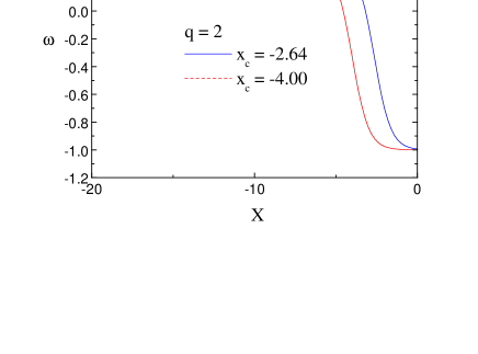
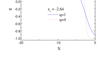
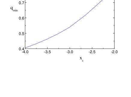
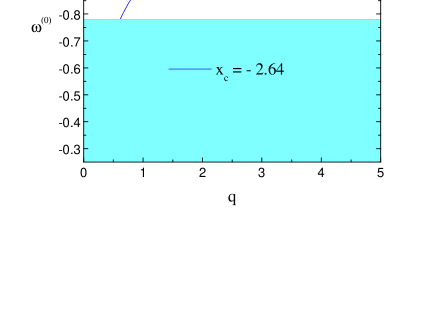
There remain two arbitrary constants $a_{c}$ and $q$, which describe the scale factor at changeover and the duration of it respectively. When $a$ is close to $a_{c}$, $\omega$ starts to decrease and $\omega$ reaches to $-1$ as $a$ approaches $a^{0}=1$. We call a transition of $\omega$ from the tracking region to the $\omega\sim-1$ region as changeover. We can also narrow the range of the $a_{c}$ value, when we consider the fact that initial value of $\rho_{\phi}$ is expected to be $120$ orders of magnitude larger than the present value. We will see this in the next section. As we can see in Eq. (2.2), for larger value of $q$, the duration of changeover of $\omega$ decreases. During early times $\omega\simeq\omega_{r}$ and it stays with same value before $a$ approaches $a_{c}$. $\omega$ will approach $\omega_{r}\times\omega_{0}$ when $a\gg a_{c}$. This is the reason we choose the values in (2.3). If $a_{c}$ is too close to $a^{(0)}=1$, then the present value of $\omega$ will not be close to $-1$ for small $q$. Thus there is a limit to $x_{c}$ for each value of $q$. The cosmological evolution of $\omega$ due to this parametrization for different values of $q$ and $x_{c}$ are shown in Fig. 1 and Fig. 2. The effect of $x_{c}$ on the evolution of $\omega$ is shown in Fig. 1 (a). A smaller value of $x_{c}$ gives an earlier change of $\omega$. As $x_{c}$ decreases, the period of $\omega=-1$ increases. A smaller value of $q$ shows a slower change of $\omega$ as in Fig. 1(b). For a specific value of $x_{c}=-2.64$, we require $q\geq 0.62$ to satisfy WMAP data. For larger values of $q$ we can still get $\omega^{(0)}=-1$ even with large $x_{c}$ (i.e. the duration of changeover is small). From Fig. 2 we show the minimum value of $q$ ($q_{\rm{min}}$) for each $x_{c}$ to satisfy WMAP data ($\omega^{(0)}<-0.78$). For a smaller value of $x_{c}$ we allow a smaller value of $q_{\rm{min}}$ to satisfy WMAP due to the fact that $\omega$ changes early and it takes more time for $\omega$ to reach today when $x_{c}$ is small. This is shown in Fig. 2(a). We also show the restriction of $q$ for a specific value of $x_{c}$ in Fig. 2(b). The advantages of this parametrization are its simplicity and the possibility of mimicking various models. However this parametrization cannot account for an oscillating $\omega$, which can be obtained from a $\cosh(\phi)$-potential and the coupled cases with general potentials [15, 16]. Thus this parametrization is good only for monotonically varying $\omega$.

Figure 1: The evolution of $\omega$. (a) The dependence on the changeover scale, $x_{c}$ of the evolution of $\omega$. A smaller value of $x_{c}$ means an earlier change of $\omega$ shown as the dashed line. (b) The dependence on $q$ of the evolution of $\omega$. The solid line ($q=1$) shows a slower change than the dashed one ($q=4$). That means the duration of the changeover becomes longer as the value of $q$ becomes smaller.

Figure 2: The present value of the equation of state, $\omega^{(0)}$. (a) $q_{\rm{min}}$ means the minimum value of $q$ for each different value of $x_{c}$ to satisfy WMAP data ($\omega^{(0)}<-0.78$) [9]. (b) The shaded region is forbidden from WMAP. From this we can make the restriction $q\geq 0.62$ when $x_{c}=-2.64$. The reason for the choice of this specific value of $x_{c}$ will be shown later.

3 CMB peak spacing

The location of the acoustic peaks and the spacing between the peaks can be estimated if an adiabatic initial condition and a flat universe are assumed [5, 17]. The acoustic scale, $l_{A}$ is given by the simple formula

$$l_{A}\equiv\pi\frac{d_{A}}{s}=\pi\frac{\tau_{0}-\tau_{ls}}{s}=\pi\frac{\tau_{0}-\tau_{ls}}{\bar{c}_{s}\tau_{ls}}$$ (3.1)

where $d_{A}$ is the angular size distance to decoupling, $\tau_{0}$ and $\tau_{ls}$ are the conformal time today and at last scattering. The sound horizon at decoupling is given by $s=\bar{c}_{s}\tau_{ls}$ and the average sound speed before last scattering is,

$$\bar{c}_{s}=\frac{\int_{0}^{\tau_{ls}}c_{s}d\tau}{\tau_{ls}}~{}~{}{\rm where}~{}~{}c_{s}^{-2}=3+\frac{9}{4}\frac{\rho_{b}(t)}{\rho_{r}(t)}$$ (3.2)

where $\rho_{b}$ and $\rho_{r}$ are the baryon and photon energy densities, respectively. The location of the $m$-th peak and trough is slightly shifted by driving effects and this can be written as [18] ;

$$l_{m}\equiv l_{A}(m-\varphi_{m})\equiv l_{A}(m-\bar{\varphi}-\delta\varphi_{m})$$ (3.3)

where $\bar{\varphi}\equiv\varphi_{1}$ is the overall peak shift and $\delta\varphi_{m}$ is the shift of the $m$-th peak relative to the first. We attach the fitting formulae in the appendix for the sake of completeness. To see the effect of quintessence, we start from the Friedmann equation.

$$H^{2}=\frac{1}{3\bar{M}^{2}}(\rho_{\phi}+\rho_{r}+\rho_{m})\equiv\frac{1}{3\bar{M}^{2}}\rho_{cr}$$ (3.4)

where $H$ is the Hubble expansion rate, $\bar{M}^{2}=M_{p}^{2}/8\pi$ is a reduced Planck mass, and $\rho_{i}$ are the energy densities of each component. From the continuity equation of energy density we find,

$$d\ln\rho_{\phi}=-3(1+\omega)dx.$$ (3.5)

This equation can be integrated using the parametrization of $\omega$ in Eq. (2.2) :

$$\rho_{\phi}(x)=\rho_{\phi}^{(0)}\exp(-4x)\Biggl{(}\frac{\exp(qx)+\exp(qx_{c})}{1+\exp(qx_{c})}\Biggr{)}^{4/q}=\rho_{\phi}^{(0)}a^{-4}\Biggl{(}\frac{a^{q}+a_{c}^{q}}{1+a_{c}^{q}}\Biggr{)}^{4/q}$$ (3.6)

where $\rho_{\phi}^{(0)}$ is the dark energy density today. We also find the dark energy density contrast ($\Omega_{\phi}$) from the above equation (3.6).

$$\Omega_{\phi}(a)=\frac{\rho_{\phi}}{\rho_{cr}}=\Biggl{[}1+\frac{\Omega_{m}^{(0)}}{\Omega_{\phi}^{(0)}}(a+a_{eq})\Biggl{(}\frac{a^{q}+a_{c}^{q}}{1+a_{c}^{q}}\Biggr{)}^{-4/q}\Biggr{]}^{-1}$$ (3.7)

where $\Omega_{i}^{(0)}=\rho_{i}^{(0)}/\rho_{cr}^{(0)}$ is the present energy density contrast of each component. In the second equality we use the relation $\Omega_{r}^{(0)}=\Omega_{m}^{(0)}a_{eq}$ where $a_{eq}$ is the scale factor when the radiation and matter densities are equal.

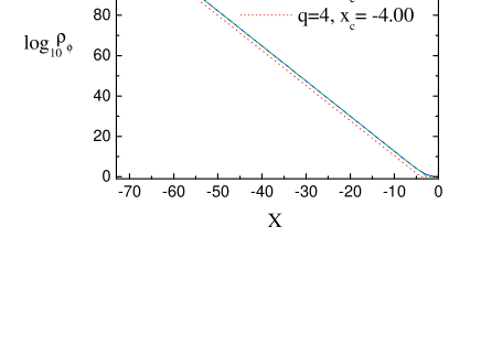
Table 1: Cosmological parameters used in the analysis. We use WMAP data [9].

$\Omega_{\phi}^{(0)}$	$\Omega_{m}^{(0)}$	$\Omega_{b}^{(0)}h^{2}$	$z_{ls}$	$z_{eq}$	$n_{s}$
$0.73$	$0.27$	$0.0224$	$1089$	$3233$	$0.93$

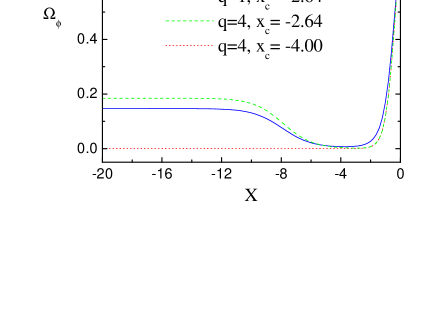
Figure 3: (a) The cosmological evolution of $\rho_{\phi}$ for specific $q$ and $x_{c}$ values. For other values of these parameters, we can get similar behaviors which can account for $120$ orders of magnitude change in $\rho_{\phi}$. (b) The evolution of $\Omega_{\phi}$ when we fix $\Omega_{\phi}^{(0)}=0.73$. When $x_{c}=-2.64$, a smaller value of $q=1$ (solid line) shows a slower change in $\Omega_{\phi}$ at late universe compared to $q=4$ (dashed line). For a smaller value of $x_{c}=-4.00$ (dotted line), $\Omega_{\phi}$ is negligible during early universe for any value of $q$.

From Eq. (3.6), we can see that the dark energy density, $\rho_{\phi}$ evolves as the energy density of radiation ($\rho_{r}\propto a^{-4}$) during $a\ll a_{c}$. $\rho_{\phi}$ starts to departure from this behavior as $a$ approaches $a_{c}$. This explains the tracking behavior of dark energy during the radiation dominated era. The cosmological evolution of the dark energy density is shown in Fig. 3. $\rho_{\phi}$ is changed by $120$ orders of magnitude through the entire history of the universe. Also from Eq. (3.6) we know that the initial value of dark energy, $\rho_{\phi}^{(0)}(a_{c}/a_{i})^{4}$ is independent of $q$, where $a_{i}$ is the scale factor at the beginning of the universe. If we use the fact that $\rho_{\phi}^{i}/\rho_{\phi}^{(0)}\sim 10^{120}$ and $a_{i}\sim 10^{-32}$, then we find that $a_{c}$ should be approximately $10^{-2}$ (equally $x_{c}\sim-4$). We can make further restriction on $a_{c}$ from the following consideration. To be compatible with observational data, the energy density of quintessence must be subdominant during Big Bang Nucleosynthesis (BBN) [3], $\Omega_{\phi}^{(BBN)}(x\sim-23)\leq 0.2$ at $T\sim 1$ MeV. If we consider the fact that $1\gg a_{c}\gg a_{eq}\gg a_{BBN}$, then the equation of dark energy density contrast (3.7) is approximately :

$$\Omega_{\phi}(a_{BBN})\simeq\Biggl{[}1+\frac{\Omega_{m}^{(0)}}{\Omega_{\phi}^{(0)}}\frac{a_{eq}}{a_{c}^{4}}\Biggr{]}^{-1}\leq 0.2\Longrightarrow a_{c}\simeq\Biggl{(}\frac{1-\Omega_{\phi}^{(0)}}{\Omega_{\phi}^{(0)}}\frac{\Omega_{\phi}^{(BBN)}}{1-\Omega_{\phi}^{(BBN)}}a_{eq}\Biggr{)}^{1/4}\leq 0.073$$ (3.8)

This corresponds to $x_{c}\leq-2.60$ independent of $q$. As previously mentioned, the slope of $\rho_{\phi}$ during the radiation dominated era has nothing to do with $a_{c}$ or $q$. The effect of $q$ appears when $a$ approaches $a_{c}$. This effect on $\rho_{\phi}$ is hardly seen as in Fig. 3(a) due to degeneracy. However we can see this effect from Fig. 3(b). A larger value of $q$ (dashed line) gives the steeper change in $\rho_{\phi}$ and $\Omega_{\phi}$ than those of a smaller value of $q$ (solid line) at late time. As we can see in the equation (3.8), the $\Omega_{\phi}$ value depends only on $a_{c}$ before $a$ reaches to $a_{eq}$. Thus for the smaller value of $a_{c}$, $\Omega_{\phi}$ value will be more close to the value of cosmological constant, $\Omega_{\Lambda}$. The evolution of dark energy density shows degeneracy between the different choice of parameters on $\omega$. This may require additional experimental data to investigate the evolution of $\omega$ instead of using SNe. Because SNe data is analyzed by the luminosity distance, which mainly depends on $\rho_{\phi}$. In the above graphs we fix $\Omega_{\phi}^{(0)}=0.73$. Now we rewrite the equation (3.4) by using conformal time, $\tau$ :

$$\Biggl{(}\frac{da}{d\tau}\Biggr{)}^{2} = H_{0}^{2}\Biggl{\{}\Omega_{r}^{(0)}+\Omega_{m}^{(0)}a+\Omega_{\phi}^{(0)}\Bigl{(}\frac{a^{q}+a_{c}^{q}}{1+a_{c}^{q}}\Bigr{)}^{4/q}\Biggr{\}}=H_{0}^{2}\Biggl{\{}\Omega_{m}^{(0)}(a+a_{eq})+\Omega_{\phi}^{(0)}\Bigl{(}\frac{a^{q}+a_{c}^{q}}{1+a_{c}^{q}}\Bigr{)}^{4/q}\Biggr{\}}$$ (3.9)

$$= H_{0}^{2}\Biggl{\{}(1-\Omega_{r}^{(0)}-\Omega_{\phi}^{(0)})(a+a_{eq})+\Omega_{\phi}^{(0)}\Bigl{(}\frac{a^{q}+a_{c}^{q}}{1+a_{c}^{q}}\Bigr{)}^{4/q}\Biggr{\}}$$

where $H_{0}$ is the present value of Hubble parameter. If we use WMAP data $\Omega_{r}^{(0)}\simeq 4.9\times 10^{-5}$, $\Omega_{m}^{(0)}\simeq 0.27$, $\Omega_{\phi}^{(0)}\simeq 0.73$, and $a_{eq}=1/(1+z_{eq})=1/3234$, then we have the following approximation of the above equation (3.9).

$$\Biggl{(}\frac{da}{d\tau}\Biggr{)}^{2}\simeq H_{0}^{2}\Biggl{\{}(1-\Omega_{\phi}^{(0)})(a+a_{eq})+\Omega_{\phi}^{(0)}\Bigl{(}\frac{a^{q}+a_{c}^{q}}{1+a_{c}^{q}}\Bigr{)}^{4/q}\Biggr{\}}\neq H_{0}^{2}\Biggl{\{}(1-\Omega_{\phi}^{(0)})a+\Omega_{\phi}^{(0)}\Bigl{(}\frac{a^{q}+a_{c}^{q}}{1+a_{c}^{q}}\Bigr{)}^{4/q}\Biggr{\}}$$ (3.10)

The approximation comes from the fact that $\Omega_{r}^{(0)}\ll\Omega_{m,\phi}^{(0)}$. We indicate the inequality between the first and the second expressions, which is frequently used in the literature. The numerical difference between two expressions is not negligible for the specific values of $a_{c}$ and $q$. So we will use the first (accurate) expression in the following calculations. From this equation we can find the numerical value of $\tau$ when $a_{c}$ and $q$ are fixed.

$$d\tau=H_{0}^{-1}\Biggl{(}(1-\Omega_{\phi}^{(0)})(a+a_{eq})+\Omega_{\phi}^{(0)}\Bigl{(}\frac{a^{q}+a_{c}^{q}}{1+a_{c}^{q}}\Bigr{)}^{4/q}\Biggr{)}^{-1/2}da$$ (3.11)

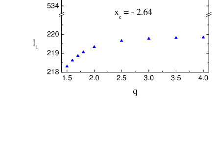
Figure 4: The locations of the first and the second CMB peaks. The uptriangles indicate the first peaks, $l_{1}$ and the downtriangles show the second peaks, $l_{2}$ as a function of $q$. Both $l_{1}$ and $l_{2}$ converge as $q$ increases.

Table 2: The spacing and the location of the CMB peaks for several values of $q$ when $x_{c}=-2.64$. Here we use the cosmological parameters in Table 1.

$x_{c}$	$q$	$l_{A}$	$l_{1}$	$l_{2}$	$\Omega_{\phi}^{ls}(10^{-2})$
$-2.64$	$1.5$	$300.8$	$218.3$	$535.0$	$5.17$
	$2$	$302.4$	$219.3$	$537.7$	$5.36$
	$3$	$303.1$	$219.8$	$538.9$	$5.40$
	$4$	$303.1$	$219.8$	$539.0$	$5.41$

By using the above equations we can find the acoustic scale ($l_{A}$), the locations of the first two peaks ($l_{1},l_{2}$), and $\Omega_{\phi}$ at last scattering ($\Omega_{\phi}^{ls}$). They are given in Table 2 and Fig. 4. For a value of $x_{c}$, the location of CMB peaks depends on $q$-values. However CMB peak values converge to some values as $q$ increases. From WMAP measurements the acoustic scale and the locations of the first two peaks are [9] :

$$l_{A}=301\pm 1,\hskip 14.45377ptl_{1}=220.1\pm 0.8,\hskip 14.45377ptl_{2}=546\pm 10.$$ (3.12)

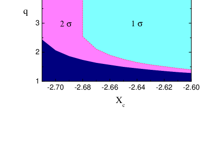
Figure 5: The $68$ % (light shaded) and 95 % (medium shaded) confidence allowed regions for $x_{c}$ and $q$ using WMAP data. Asterisk indicates the best fit values ($x_{c}=-2.64$, $q=4.01$). The dark shaded regions are out of $2\sigma$ confidence level. The constraint from the dark energy density at BBN determines the upper limit on $x_{c}\,(\leq-2.60)$. The lower limit of $x_{c}\,(>-2.72)$ is obtained from $\chi^{2}$-analysis. There is no upper limit on $q$ values from WMAP. However we can obtain the upper limit on $q$ from the analysis of the time varying $\alpha$ in the following section.

If we assume that the errors are Gaussian and uncorrelated, then we can find a $\chi^{2}$-statistic

$$\chi^{2}=\sum_{i}\frac{\Bigl{(}l_{i,obs}-l_{i,theory}\Bigr{)}^{2}}{\sigma_{i}^{2}}$$ (3.13)

where $l_{i,obs}$ is the observational data of each peak, $l_{i,theory}$ is the theoretical value of $l_{i}$, and $\sigma_{i}$ is the statistical uncertainty for each peak. The likelihoods for the parameters ($q,x_{c}$) of the parametrization given in (2.2) are calculated from $\chi^{2}$ so that the $68$ % and $95$ % confidence regions are determined by $\Delta\chi^{2}\equiv\chi^{2}-\chi_{0}^{2}=2.30$ and $6.17$ respectively. $\chi_{0}^{2}$ is $\chi^{2}$ for the best fit model found. The best fit values to the WMAP data is obtained from $x_{c}=-2.64$ and $q=4.01$. The likelihood contours for WMAP are shown in Fig. 5. The $68$ % (light shaded) and 95 % (medium shaded) confidence allowed regions for $x_{c}$ and $q$ are shown using WMAP data. There is no upper limit on $q$ values for several $x_{c}$ values. From this we find at $95$ % CL :

$$\omega^{(0)}\leq-0.971_{-0.027}^{+0.017}~{},\hskip 14.45377pt\Biggl{(}\frac{d\omega}{dz}\Biggr{)}_{z=0}\leq 0.041_{-0.037}^{+0.016}$$ (3.14)

$\omega$ is almost a constant at present, which is consistent with recent observation [19].

4 Time variation of the fine structure constant

In this section we consider the $\phi$-dependence of the gauge couplings in Standard Model (SM), $B_{F}(\phi)$ [16]. The interaction of a light scalar field $\phi$ with electromagnetic field is represented in the Lagrangian as ${\cal L}_{EM}=-B_{F}(\phi)F_{\mu\nu}F^{\mu\nu}/4$, where $F^{\mu\nu}$ is the electromagnetic field-strength tensor. The main assumption in this work is that all functions $B_{F}(\phi)$ and $V(\phi)$ admit a common extremum, which is a generalization of Damour-Nordtvedt and Damour-Polyakov constructions [20]. To this end, we proposed an ansatz that would relate $B_{F}(\phi)$ and $V(\phi)$.

$$B_{F}(\phi)=\Biggl{(}\frac{b_{F}+V(\phi)/V_{0}}{1+b_{F}}\Biggr{)}^{n_{F}},~{}~{}~{}{\rm where}~{}~{}b_{F}+1>0$$ (4.1)

where $n_{F}$ and $b_{F}$ are two dimensionless parameters allowing us to cover a wide range of possibilities. We will assume that dark energy is a quintessence field and its potential is parameterized by $\omega$. So instead of introducing a potential of the scalar field, we will use $\omega$. We can rewrite (4.1) by using the parametrization of $\omega$ (2.2). We also use the relation between the potential $V(\phi)$ and the energy density $\rho_{\phi}$ of the scalar field,

$$V(\phi)=\frac{(1-\omega)}{2}\rho_{\phi}\Rightarrow V(x)=\rho_{\phi}^{(0)}\exp(-4x)A_{1}(x)A_{2}(x)$$ (4.2)

where

$$A_{1}(x) = \Biggl{(}\frac{\exp(qx)+\exp(qx_{c})}{1+\exp(qx_{c})}\Biggr{)}^{4/q}~{},$$ (4.3)

$$A_{2}(x) = \frac{3\exp(qx)+\exp(qx_{c})}{3\Bigl{(}\exp(qx)+\exp(qx_{c})\Bigr{)}}$$ (4.4)

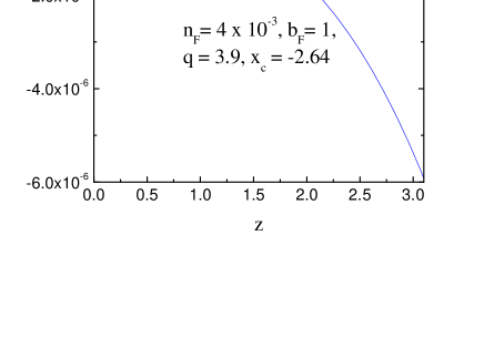
Figure 6: A typical evolution $\Delta\alpha/\alpha$ for specific $n_{F}$, $b_{F}$, $q$ and $x_{c}$ values. We can get similar behaviors with other values of parameters. $n_{F}$ and $b_{F}$ values are obtained from the result of Murphy et al. Several values of $\Delta\alpha/\alpha$ for various choices of the parameters at different $z$ are indicated in Table 3.

With these equations (2.2), (3.6), and (4.2), we can rewrite the gauge coupling in Eq (4.1) as follow,

$$B_{F}(x)=\Biggl{(}\frac{b_{F}+\exp(-4x)A_{1}(x)A_{2}(x)/A_{2}(0)}{1+b_{F}}\Biggr{)}^{n_{F}}$$ (4.5)

where we assume that $V_{0}=V(x=0)$ to satisfy $B_{F}(0)=1$. We can find the time variation of the fine structure constant by using the following relation between $B_{F}$ and $\alpha$,

$$\frac{\Delta\alpha}{\alpha}\equiv\frac{\alpha(x)-\alpha(0)}{\alpha(0)}=\frac{1}{B_{F}(x)}-1.$$ (4.6)

From equations (4.5) and (4.6), we find

$$\frac{\Delta\alpha}{\alpha}=\Biggl{(}\frac{1+b_{F}}{b_{F}+\exp(-4x)A_{1}(x)A_{2}(x)/A_{2}(0)}\Biggr{)}^{n_{F}}-1$$ (4.7)

Table 3: The values of $\Delta\alpha/\alpha$ at the different $z$ for the several values of $q$ when $x_{c}=-2.64$. Here we use the QSOs result to fix other values [21]. $n_{F}$ has been scaled by a factor of $10^{3}$, $\Delta\alpha/\alpha$ values have been scaled by a factor of $10^{6}$ except the value at decoupling $(\Delta\alpha/\alpha)_{ls}$, which is given in the last column without any scaling.

$x_{c}$	$q$	$n_{F}$	$b_{F}$	$(\frac{\Delta\alpha}{\alpha})_{3}$	$(\frac{\Delta\alpha}{\alpha})_{1.5}$	$(\frac{\overline{\Delta\alpha}}{\alpha})_{0.45}$	$(\frac{\Delta\alpha}{\alpha})_{0.14}$	$(\frac{\Delta\alpha}{\alpha})_{1089}$
$-2.64$	$3$	$4.25$	$11$	$-5.4$	$-1.25$	$-0.017$	$-0.041$	$-0.057$
		$0.71$	$1$	$-5.4$	$-1.26$	$-0.017$	$-0.042$	$-0.011$
	$3.5$	$3.68$	$3$	$-5.4$	$-1.01$	$-0.023$	$-0.025$	$-0.053$
		$1.84$	$1$	$-5.4$	$-1.01$	$-0.023$	$-0.025$	$-0.028$
	$3.9$	$4.01$	$1$	$-5.4$	$-0.84$	$-0.016$	$-0.016$	$-0.060$

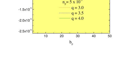
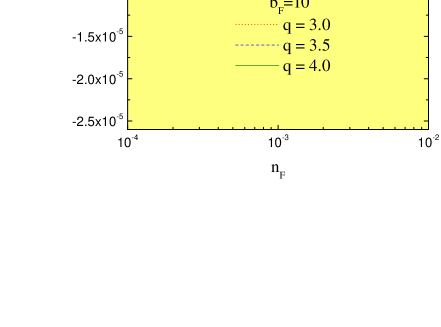
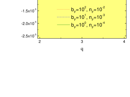
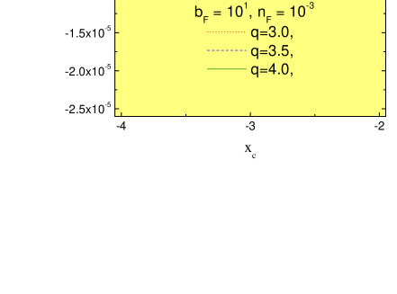
Figure 7: The cosmological evolution of $\alpha$ for the various parameters. Murphy et al data (medium shaded) is used in all of the figures, $(\Delta\alpha/\alpha)_{z=3}=(-0.543\pm 0.116)\times 10^{-6}$. We use $x_{c}=-2.64$ for all of the graphs except (d). (a) The evolution of $\Delta\alpha/\alpha$ with respect to $b_{F}\geq 1$ for $n_{F}=5\times 10^{-3}$. When $q=3$ (dotted line) $\alpha$ changes slower than when $q=4$ (solid line). Thus we have more acceptable values of $b$ for the smaller $q$ ($10.6\leq b_{F}\leq 16.9$ when $q=3$). (b) The effect of changing $n_{F}$ on $\Delta\alpha/\alpha$ while we fix $b_{F}=10$. (c) and (d) the effect of varying $q$ and $x_{c}$ on the variation of $\alpha$, respectively.

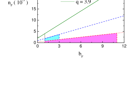
In Table 3, we display $\Delta\alpha/\alpha$ values at different redshifts for the various parameters. Especially we show specific results for $x_{c}=-2.64$, because this gives the best-fit value for the separation of CMB peaks as explained in the previous section. $\Delta\alpha/\alpha$ at the cosmic microwave background epoch, which is constrained as $(\Delta\alpha/\alpha)_{ls}\geq-0.06$ [22] are shown in the last column. There are four parameters ($n_{F},b_{F},x_{c}$, and $q$) to be fixed. In Fig. 6 we show a typical evolution of $\Delta\alpha/\alpha$ for a specific set of four parameters (i.e. $n_{F}=4\times 10^{-3}$, $b_{F}=1$, $q=3.9$, and $x_{c}=-2.64$). We can change four parameters to explain the effect on the evolution of $\alpha$. However it is impossible to fix all four parameters at once. Thus we show the effect of the changing each parameter with fixing all other parameters at each time. We see that smaller values of $q$ lead to more room for the parameter space regions of $n_{F}$ and $b_{F}$, because smaller values of $q$ lead to slower change in $\alpha$. For given $q$-values, there may not be any solution to fit experimental data as shown in the first panel of Fig. 7. However as we increase the $b_{F}$-values we can satisfy the experimental data. We have larger $b_{F}$ range for smaller values of $q$. Similar consideration can be made for varying $n_{F}$. For example, even though the dotted lines (q = 3) in the second panel does not fit experimental data when $n_{F}\geq 3\times 10^{-3}$, as we decrease $n_{F}$ we can recover the suitable $\Delta\alpha/\alpha$ for given $q$ and $x_{c}$. The medium shaded regions of each panel are allowed from Murphy et al, ($\Delta\alpha/\alpha)_{z=3}=(-0.543\pm 0.116)\times 10^{-5}$ [21]. The effect of changing $q$ and $x_{c}$ are shown in $(c)$ and $(d)$ of Fig. 7. As we expect there is lots of room for the choice of $q$ and $x_{c}$ because we have extra degrees of freedom ($n_{F}$ and $b_{F}$) to be fixed in addition to the original parameters of $\omega$. However combined with the analysis of the separation of CMB peaks, the parameters on gauge coupling are much narrowed as in Table 3. We can make the allowed regions for $n_{F}$ and $b_{F}$ from the narrowed parameter spaces of $a_{c}$ and $q$. This is indicated in Fig. 8. The sloped lines are obtained from the normalization of Murphy et al data for the given $q$ values when $x_{c}$ is fixed as $-2.64$. The vertical lines for each $q$ come from both the CMB bound on $\alpha$ and the assumption of $b\geq 1$. There is only one allowed value $b_{F}=1$ for $q=3.9$ ( solid line ). This gives the upper limit on $q\leq-3.9$, which we can use for the consideration of CMB peaks. For $q=3$ (dotted line), there are more parameter spaces to satisfy the constraints. In this case $b_{F}$ can be increased up to $11$. Obviously this gives much narrower parameter spaces for each parameter compared to Fig. 7. Now we can restrict ($n_{F},b_{F}$) $\sim$ ($10^{-3},1$) as in [16] and $1.5\leq q\leq 3.9$ for $x_{c}=-2.64$.

Figure 8: The constraints on $n_{F}$ and $b_{F}$ from both the result of Murphy et al [21] and that of CMB [22]. $n_{F}$ values in the graph are scaled by $10^{3}$. The sloped lines are obtained from QSOs result. The vertical line for each case is obtained from CMB. The shaded regions are allowed ones from both constraints. There is only one $b_{F}$-value for $q=3.9$ (solid line) when we assume that $b\geq 1$. So we can get the upper limit $q<4$.

5 Conclusions

We have introduced a simple parametrization of $\omega$ based on both theory and experiment. A tracking solution is proposed to alleviate the fine tuning problem and the present value of $\omega$ is observed to be close to $-1$. We have analyzed the separation of CMB peaks and the time variation of the fine structure constant with this parametrization. We have obtained the constraints of the parameters of $\omega$ from these analyses which use both low-redshifts and high-redshifts data. We have been able to use the analytically integrated value of the dark energy density contrast, $\Omega_{\phi}$ from this parametrization.

From WMAP data, we have obtained a very specific value of $x_{c}\sim-2.64$ (equally $z_{c}\sim 13$) for the best fit value. When $x_{c}=-2.64$ we have obtained the very small $(dw/dz)_{z=0}$, which is consistent with the recent observations. $(dw/dz)$ depends on $x_{c}$, which is related to the epoch when the time evolution of $\omega$ begins. A smaller value of $x_{c}$ causes an earlier evolution of $\omega$ compared to a larger value of $x_{c}$. With a smaller $x_{c}$, $\rho_{\phi}$ evolves to its present value $\rho_{\phi}^{(0)}$ at an early epoch and it stays with this value because $\omega\sim-1$. In this case $\Omega_{\phi}$ is negligible until it reaches its present value and that is similar to when we have the cosmological constant as dark energy. However for some values of $x_{c}$ the value of $\Omega_{\phi}$ can be significant at early times. This behavior is quite different from that of a cosmological constant. Thus the difference between the cosmological constant and quintessence is obvious for some values of $x_{c}$. Due to CMB consideration we have focused on $x_{c}=-2.64$ and this has shown the big discrepancy between quintessence and the cosmological constant. We have also found that to be consistent with BBN (i.e. $\Omega_{\phi}^{(BBN)}\leq 0.18$) we need $q\geq 1.50$ when $x_{c}=-2.64$. Thus this may give one clue for the nature of dark energy. We have made the restriction to the value of $q$, $q_{\rm{min}}$ from the constraint on $x_{c}$. As $x_{c}$ increases, we will get bigger $q_{\rm{min}}$ as in Fig. 2. We have also found the upper limit on $x_{c}$ when we consider the limit of $\Omega_{\phi}^{(BBN)}$, $x_{c}\leq-2.60$. We have reached to the lower limit $q\geq 1.50$ when we used $\Omega_{\phi}^{ls}\sim 0.01$ from WMAP. We have had the similar lower limit on $q$ from the $\chi^{2}$-statistic. All of this consideration gives the unique lower limit of $q\geq 1.50$ when we choose $x_{c}=-2.64$ However there was no upper limit of $q$ from the CMB analysis alone.

We have introduced two more parameters ($n_{F},b_{F}$) from the generic form of gauge coupling to analyze the evolution of $\Delta\alpha/\alpha$. However we had only three parameters to be fixed after specifying $x_{c}$. We have found the viable parameter regions for each parameter by using $\Delta\alpha/\alpha$ data. From this we have found the well known parameter regions of gauge coupling $(n_{F},b_{F})\sim(10^{-3},1)$ [16]. We have also found the upper limit $q\leq 3.90$ with this analysis.

We have found a viable parametrization of $\omega$ with the very specific parameter regions, $x_{c}=-2.64$ and $1.50\leq q\leq 3.90$ from the analyses of both the separation of CMB peaks and the time variation of $\alpha$. We have also found that $-1.00\leq\omega^{(0)}\leq-0.971_{-0.027}^{+0.017}$ and $1.76_{-0.42}^{+0.29}\times 10^{-4}\leq(d\omega/dz)_{z=0}\leq 0.041_{-0.037}^{+0.016}$ at $95$ % CL. Thus we may not see any change of $\omega$ at present. Even though the present values of $\omega$ and $d\omega/dz$ are almost identical to the values of the cosmological constant, $\Omega_{\phi}$ evolves from BBN to the present with significant values. Thus this model has the different cosmological behaviors compared to $\Lambda$CDM model. We may need to check the similar parametrization and/or more data to investigate the nature of dark energy. We may also need to modify $\omega$ to have more than one changeover which can show a non-monotonic behavior.

6 Acknowledgements

This work was supported in part by DOE grant DE-FG02-94ER-40823. We would like to thank Keith.A. Olive for useful discussion.

Appendix A Appendix

We have used the analytic approximations for the phase shifts Doran, which we show here. The overall phase shift is given by

$${\bar{\varphi}}=(1.466-0.466n_{s})\left[a_{1}r_{*}^{a_{2}}+0.291{\bar{\Omega}}_{\phi}^{ls}\right]$$ (A.1)

where the fitting coefficients are

$$a_{1} = 0.286+0.626\omega_{b}$$

$$a_{2} = 0.1786-6.308\omega_{b}+174.9\omega_{b}^{2}-1168\omega_{b}^{3}$$ (A.2)

with $\omega_{b}=\Omega_{b}^{(0)}h^{2}$, and ${\bar{\Omega}}_{\phi}^{ls}$ is given by

$${\bar{\Omega}}_{\phi}^{ls}=\tau_{ls}^{-1}\int_{0}^{\tau_{ls}}\Omega_{\phi}(\tau)d\tau$$ (A.3)

and

$$r_{*}\equiv\rho_{r}(z_{ls})/\rho_{m}(z_{ls})$$ (A.4)

is the ratio of radiation to matter at decoupling. The relative shift of the first acoustic peak is zero, $\delta\varphi_{1}=0$, and the relative shifts of the second peak are given by

$$\delta\varphi_{2}=c_{0}-c_{1}r_{*}-c_{2}r_{*}^{-c_{3}}+0.05(n_{s}-1)~{}$$ (A.5)

where $n_{s}$ is scalar spectral index and

$$c_{0} = -0.1+\left(0.213-0.123{\bar{\Omega}}_{ls}^{\phi}\right)\times\exp\Bigl{(}-[52-63.6{\bar{\Omega}}_{ls}^{\phi}]\omega_{b}\Bigl{)}$$

$$c_{1} = 0.015+0.063\exp\left(-3500\omega_{b}^{2}\right)$$

$$c_{2} = 6\times 10^{-6}+0.137(\omega_{b}-0.07)^{2}$$

$$c_{3} = 0.8+2.3{\bar{\Omega}}_{ls}^{\phi}+\left(70-126{\bar{\Omega}}_{ls}^{\phi}\right)\omega_{b}$$ (A.6)

References

• [1] A. G. Riess et al. [Supernova Search Team Collaboration], Astron. J.  116 (1998) 1009 [arXiv:astro-ph/9805201]; S. Perlmutter et al. [Supernova Cosmology Project Collaboration], Astrophys. J.  517 (1999) 565 [arXiv:astro-ph/9812133]; N. A. Bahcall, J. P. Ostriker, S. Perlmutter and P. J. Steinhardt, Science 284 (1999) 1481 [arXiv:astro-ph/9906463].
• [2] B. Ratra, P.J.E. Peebles, Phys. Rev. D 37, 3406 (1988); Ap. J. Lett 325, 117 (1988); C. Wetterich, Nucl. Phys. B 302, 668 (1988); R.R. Caldwell, R. Dave and P.J. Steinhardt, Phys. Rev. Lett 80, 1582 (1998) [astro-ph/9708069].
• [3] P.G. Ferreira and M. Joyce, Phys. Rev. D 58, 023503 (1998) [astro-ph/9711102].
• [4] E.V. Linder and R. Miquel, [astro-ph/0409411].
• [5] T.Barreiro, M.C. Bento, N.M.C. Santos, and A.A. Sen, Phys. Rev. D 68 043515 (2003) [astro-ph/0303298]; W. Hu, Annals Phys, 303 (2003) 203 [astro-ph/0210696]; M.C. Bento, O. Bertolami, and A.A. Sen, Phys. Rev. D 67 063003 [astro-ph/0210468]; M. Doran, M. Lilley, J. Schwindt, and C. Wetterich, Astrophys. J. 599 (2001) 501 [astro-ph/0012139];.
• [6] N.J. Nunes and J.E. Lidsey, Phys. Rev. D 69 123511 (2004) [astro-ph/0310882]; D. Parkinson, B.A. Bassett, and J.D. Barrow, Phys. Lett. B 578, 235 (2004) [astro-ph/0307227].
• [7] I. Maor, R. Brustein, and P.J. Steinhardt, Phys. Rev. Lett. 86, 6 (2001); Erratum ibid. 87 049901 (2001) [astro-ph/0007297].
• [8] S. Hannestad and E. Mortsell, JCAP, 0409 (2004) 001 [astro-ph/0407259].
• [9] D.N. Spergel et al., Astrophys. J. Suppl 148 (2003) 175 [astro-ph/0302209].
• [10] E. Linder, Phys. Rev. D 70, 023511 (2004) [astro-ph/0402503]; H.K. Jassal, J.S. Bagla, and T. Padmanabhan, [astro-ph/0404378].
• [11] U. Alam, V. Sahni, T.D. Saini, and A.A. Starobinsky, Mon. Not. Roy. Astron. Soc. 354 (2004) 275 [astro-ph/0311364]; C. Wetterich, Phys. Lett. B 594 (2004) 17 [astro-ph/0403289]; P.S. Corasaniti et al, Phys. Rev. D 70, 083066 (2004) [astro-ph/0406608].
• [12] B. Boisseau, G. Esposito-Farese, D. Polarski, and A.A. Starobinsky; Phys. Rev. Lett 85 2236 (2000) [gr-qc/0001066].
• [13] R.R. Caldwell; Phys. Lett. B 545 (2002) 23 [astro-ph/9908168].
• [14] A. Lue and G.D. Starkman, Phys. Rev. D 70 101501 (2004) [astro-ph/0408246].
• [15] V. Sahni and L. Wang, Phys. Rev. D bf 62 103517 (2000) [astro-ph/9910097].
• [16] S. Lee, K.A. Olive, and M. Pospelov, Phys. Rev. D 70 083503 (2004) [astro-ph/0406039].
• [17] W. Hu, N. Sugiyama, and J. Silk, Nature 386 (1997) 37 [astro-ph/9604166].
• [18] W. Hu, M. Fukugita, M. Zaldarriaga, and M. Tegmark, Astrophys. J 549 (2001) 669 [astro-ph/0006436]; M. Doran and M. Lilley, Mon. Not. Roy. Astron. Soc 330 965 (2002) [astro-ph/0104486].
• [19] A.G. Riess et al., Astrophys. J. 607 (2004) 665 [astro-ph/0402512].
• [20] T. Damour and K. Nordtvedt, Phys. Rev. Lett. 70, 2217 (1993); Phys. Rev. D. 48, 3436 (1993); T. Damour and A.M. Polyakov, Nucl. Phys. B423, 532 (1994) [hep-th/9401069]; Gen. Relativ. Gravit. 26, 1171 (1994) [gr-qc/9411069].
• [21] J. K. Webb et al., Phys. Rev. Lett.  87, 091301 (2001) [arXiv:astro-ph/0012539]; M. T. Murphy, J. K. Webb and V. V. Flambaum, Mon. Not. Roy. Astron. Soc.  345, 609 (2003) [arXiv:astro-ph/0306483].
• [22] G. Rocha, R. Trotta, C. J. A. Martins, A. Melchiorri, P. P. Avelino and P. T. P. Viana, New Astron. Rev.  47, 863 (2003) [arXiv:astro-ph/0309205].