An Analytic Model for the Axis-Ratio Distribution of Dark Matter Halos from the Primordial Gaussian Density Field

Abstract

We present an analytic expression for the axis ratio distribution of triaxial dark matter halos driven from physical principles. Adopting the picture of triaxial collapse based on the Zel’dovich approximation, we derive analytically both the minor-to-major and the conditional intermediate-to-major axis ratio distributions, and examine how they depend on the halo mass, redshift, and cosmology. Our analytic model is tested against the simulation data given by Jing & Suto in 2002, and found to reproduce the conditional intermediate-to-major axis ratio distribution successfully and the minor-to-major axis ratio distribution approximately. However, the trends of our analytic axis-ratio distributions with mass and redshift are opposite to what is found in N-body simulations. This failure of our analytic model puts a limitation on analytic approaches based on the Lagrangian theory to the halo ellipticity. Given the overall agreement with the simulation results, our model provides a new theoretical step toward using the axis-ratio distribution of dark halos as a cosmological probe. We also discuss several possibilities to improve the model.

1 INTRODUCTION

While shapes of dark matter halos have been conventionally modeled as spherical (Navaro, Frenk, & White, 1997; Moore et al., 1999), optical, X-ray and lensing observations of galaxy clusters suggest that the shapes of dark halos are far from spherical (West, 1989; Plionis, Barrow, & Frenck, 1991). Recent high-resolution simulations do indicate that the density profiles of dark halos are better approximated as triaxial (Frenk et al., 1988; Warren et al., 1992; Jing & Suto, 2002; Suwa et al., 2003; Kasun & Evrard, 2004; Hopkins, Bahcall, & Bode, 2004).

Jing & Suto (2002, JS02 hereafter) were able to construct a detailed empirical model for the triaxial halo for the first time. Their fitting model turned out to be quite useful in quantifying the triaxiality effect on many important observables such as the strong lensing arc statistics (Oguri, Lee, & Suto, 2003; Oguri & Keeton, 2004; Dalal, Holder, & Hennawi, 2004), the halo mass-temperature relation (Yang, Yu, & Shen, 2004), and the halo figure rotation (Bailin & Steinmetz, 2004).

The most fundamental statistics characterizing the halo triaxiality is the axis-ratio, or equivalently, ellipticity distribution functions. Hopkins, Bahcall, & Bode (2004) have shown from their N-body simulations that the axis-ratio distributions depend on the halo environments in addition to the underlying cosmology. In order to exploit the halo axis-ratio distribution as a cosmological probe, therefore, one needs an analytic model beyond the empirical fitting formulae. This is exactly what we attempt to propose in this paper.

In fact, the triaxial shape of a dark halo is a generic prediction of the CDM (Cold Dark Matter) paradigm. Bardeen et al. (1986) already derived an analytic expression of the halo axis-ratio distribution assuming that dark halos form at peaks of the primordial Gaussian density field. They showed theoretically that the CDM dark halos cannot be spherical as pointed out earlier by Doroshkevich (1970). However, recent numerical results mentioned above have demonstrated that simulated dark halos are even more elliptical than expected in the previous density peak approach. This is why we revisit this problem using different analytical approaches.

To construct a new theoretical model for the halo axis-ratio distribution, we adopt the cosmic web picture (Bond, Kofman, & Pogosyan, 1996) which describes one dimensional filaments in the CDM framework. According to the picture, the distribution and spatial coherence of initial tidal fields induces the filamentary pattern of the large scale structure. Later the filaments bridge between dark matter halos, and the merging of dark halos occur preferentially along the bridging filaments. Thus the resulting halos cannot be spherical but naturally become elongated along the filaments. The halo ellipticities are expected to increase as the hierarchical merging along the filaments proceeds. Therefore, the halo axis-ratio can be inferred statistically by combining an evolution model of non-spherical density perturbations and the primordial filamentarity of the initial density field.

In order to examine the validity of our analytical model, we compare the predictions with the simulation results by JS02. For that purpose, we consider two specific sets of cosmological parameters that they adopted. The first model is $\Lambda$CDM model which assumes that $\Omega_{m}=0.3$, $\Omega_{\Lambda}=0.7$, $\sigma_{8}=0.9$, and $\Gamma=0.2$, where $\Omega_{m}$ and $\Omega_{\Lambda}$ denote the matter density parameter and the dimensionless cosmological constant, and $\sigma_{8}$ is the amplitude of the mass fluctuation at $8h^{-1}$Mpc. Since JS02 use the CDM transfer function of Bardeen et al. (1986) neglecting the baryon contribution, the shape parameter $\Gamma$ simply equals $\Omega_{m}h$. The second model is SCDM model where $\Omega_{m}=1$, $\Omega_{\Lambda}=0$, $\sigma_{8}=0.55$, and $\Gamma=0.5$. JS02 considered dark halos consisting of more than $10^{4}$ particles. Since a mass of a simulation particle is $2.07\times 10^{9}\Omega_{m}h^{-1}M_{\odot}$ ($512^{3}$ particles in $100h^{-1}$Mpc comoving cube), it is convenient to define the dimensionless mass of $M_{4}\equiv M/(2.07\times 10^{13}\Omega_{m}h^{-1}M_{\odot})$.

The rest of this paper is organized as follows. Section 2 describes our basic assumptions in the analytic modeling. We lay out mathematical details of derivation of the axis ratio distributions in §3, and compare the analytic results with their simulation results in §4. Finally §5 is devoted to discussion and conclusions.

2 BASIC ASSUMPTIONS

To derive the axis-ratio distribution of dark matter halos, we adopt three major assumptions. First, the trajectory of a dark matter particle in the comoving coordinate is well approximated by the Zel’dovich formula (Zeldovich, 1970). According to the approximation, the key quantities are the three eigenvalues ($\lambda_{1}\geq\lambda_{2}\geq\lambda_{3}$) of the deformation tensor (or the tidal shear tensor), $d_{ij}$, which is defined as the second derivative of the perturbation potential, $\Psi$, at the initial epoch $z_{i}$:

$$d_{ij}\equiv\partial_{i}\partial_{j}\Psi.$$ (1)

The mapping from the Lagrangian to the Eulerian spaces yields an expression of the particle density $\rho$ in the Eulerian space ${\bf x}$ at redshift $z$:

$$\rho({\bf x},z)=\frac{\bar{\rho}(z)}{[1-\tilde{D}_{+}(z)\lambda_{1}][1-\tilde{D}_{+}(z)\lambda_{2}][1-\tilde{D}_{+}(z)\lambda_{3}]},$$ (2)

where $\bar{\rho}$ is the background density of the universe, and $\tilde{D}_{+}(z)\equiv D_{+}(z)/D_{+}(z_{i})$ denotes the linear growth rate of density fluctuations up to $z$ but normalized to unity at redshift $z_{i}$. Note that $\lambda_{1}$, $\lambda_{2}$, and $\lambda_{3}$ in equation (2) represent the eigenvalues of $d_{ij}$ defined at $z_{i}$. In practice, we use the following fitting formula (Peacock, 1999):

$$D_{+}(z)=\frac{5}{2}\Omega_{m}[\Omega_{m}(1+z)^{3}+\Omega_{\Lambda}]^{1/2}\int_{z}^{\infty}\frac{1+z^{\prime}}{[\Omega_{m}(1+z^{\prime})^{3}+\Omega_{\Lambda}]^{3/2}}\ dz^{\prime}.$$ (3)

The linear density contrast, $\delta$, at $z_{i}$ is simply written as

$$\delta({\bf x},z_{i})=\lambda_{1}+\lambda_{2}+\lambda_{3}.$$ (4)

Second, we assume that a dark matter halo of mass $M$ forms at redshift $z$ when the corresponding Lagrangian region (at $z_{i}$) in the linear density field smoothed over $M$ satisfies the following conditions:

$$\delta(z_{i})=\delta_{c}(z),\qquad\lambda_{3}(z_{i})\geq\lambda_{c}(z),$$ (5)

where $\delta$ and $\lambda_{3}$ are the linear density contrast and the smallest eigenvalue of $d_{ij}$ of the smoothed density field, respectively. Here $\delta_{c}(z)$ and $\lambda_{c}(z)$ are redshift-dependent threshold of $\delta$ and lower limit of $\lambda_{3}$, respectively:

$$\delta_{c}(z)=\delta_{c0}\tilde{D}_{+}(0)/\tilde{D}_{+}(z),\qquad\lambda_{c}(z)=\lambda_{c0}\tilde{D}_{+}(0)/\tilde{D}_{+}(z).$$ (6)

We use the collapse threshold $\delta_{c0}$ computed in the spherical model. For SCDM, it is $\delta_{c}\approx 1.686$. For $\Lambda$CDM, we use the formula given in Appendix B of Kitayama & Suto (1996), which depends weakly on cosmology.

In the spherical approximation, the condition of $\delta(z_{i})=\delta_{c}(z)$ is sufficient for the gravitational collapse at $z$. In the non-spherical model based on the Zel’dovich approximation, however, all regions satisfying $\delta=\delta_{c}$ do not necessarily collapse into dark halos, since $\lambda_{3}$ can be negative even when $\delta=\delta_{c}$. This is why we impose the additional condition (5) in our model based on the Zel’dovich approximation. Nevertheless no reliable modeling is known which determines the value of $\lambda_{c0}$ from physical principles. While the Zel’dovich approximation suggests $\lambda_{c0}=1$, those objects are subject to the first-shell crossing, beyond which the Zel’dovich approximation is not valid at all. Indeed, Lee & Shandarin (1998) empirically proposed a value of $\lambda_{c0}=0.37$ in their mass function theory. They argue that realistic collapse should proceed along all the three axes almost simultaneously. Thus the collapse along the major axis should be accelerated by the collapse along the other two directions, resulting in a lower value of $\lambda_{c0}$. Throughout this paper, we adopt their value of $\lambda_{c0}=0.37$ unless otherwise stated (see §3).

Third, the principal axes of the inertia tensor of a dark matter halo are aligned with that of the linear tidal shear tensor of the corresponding Lagrangian region. Approximating that the density profile of a dark matter halo as a triaxial ellipsoid with three distinct axes, $a$, $b$, and $c$ (we define $a\leq b\leq c$), one can say that the inertia shape tensor of a dark halo has three distinct eigenvalues, $a,b,c$. The three eigenvalues of the halo inertia tensor, $\{a,b,c\}$, are related to the eigenvalues of the tidal shear tensor, $\{\lambda_{1},\lambda_{2},\lambda_{3}\}$ as

$$a\propto\sqrt{1-\tilde{D}_{+}\lambda_{1}},\qquad b\propto\sqrt{1-\tilde{D}_{+}\lambda_{2}},\qquad c\propto\sqrt{1-\tilde{D}_{+}\lambda_{3}},$$ (7)

It may be interesting to compare our definition of the halo axes (eq.[7]) with that of the density peak formalism (Bardeen et al., 1986). In the density peak formalism, the three eigenvalues of the halo inertia tensor are defined as

$$a\propto\frac{1}{\sqrt{\zeta_{1}}},\qquad b\propto\frac{1}{\sqrt{\zeta_{2}}},\qquad c\propto\frac{1}{\sqrt{\zeta_{3}}},$$ (8)

where $\zeta_{1}$, $\zeta_{2}$, and $\zeta_{3}$ are the three eigenvalues of the second derivative of the linear density field, $\partial_{i}\partial_{j}\delta$. The comparison of two equations (7) and (8) shows that in the density peak formalism the inertia shape tensor of a dark halo is almost independent of the tidal shear tensor, $d_{ij}$, while in our formalism which basically assumes that the ellipticity of a dark halo is induced by the filamentary cosmic web, it is directly related with $d_{ij}$. In fact, the strong correlation between the halo inertia and the tidal shear tensors was demonstrated by recent N-body simulations (Lee & Pen, 2000; Porciani, Dekel, & Hoffman, 2002).

The above three assumptions imply that dark matter halos preferentially form at the over-dense nodes of the filamentary web of the initial density field where the principal axes of the inertia and the tidal tensors are aligned with each other. Using these simplified assumptions, we derive analytically the distribution of the axis-ratios of dark halos in the following two sections.

3 THE MINOR-TO-MAJOR AXIS RATIO DISTRIBUTION

We start from the joint probability distribution of the three eigenvalues of the tidal shear tensor in the primordial Gaussian density field (Doroshkevich, 1970):

$$p(\lambda_{1},\lambda_{2},\lambda_{3};\sigma_{M})=\frac{3375}{8\sqrt{5}\pi\sigma^{6}_{M}}\exp\bigg{(}-\frac{3I_{1}^{2}}{\sigma^{2}_{M}}+\frac{15I_{2}}{2\sigma^{2}_{M}}\bigg{)}(\lambda_{1}-\lambda_{2})(\lambda_{2}-\lambda_{3})(\lambda_{1}-\lambda_{3}),$$ (9)

where

$$I_{1}\equiv\lambda_{1}+\lambda_{2}+\lambda_{3},\qquad I_{2}\equiv\lambda_{1}\lambda_{2}+\lambda_{2}\lambda_{3}+\lambda_{3}\lambda_{1},$$ (10)

We define $\sigma_{M}$ as the rms fluctuation of the linear density field at $z_{i}$ smoothed on mass scale $M$:

$$\sigma^{2}_{M}(z_{i})=\frac{1}{(2\pi)^{3}}\int P(k,z_{i})W_{TH}^{2}(kR_{M})d^{3}k,$$ (11)

where $P(k,z_{i})$ is the linear power spectrum of the density field, and $W_{TH}(kR_{M})$ is the top-hat filter with $R_{M}\equiv[3M/(4\pi\bar{\rho})]^{1/3}$.

We change the variables from $\{\lambda_{1},\lambda_{2},\lambda_{3}\}$ to $\{\lambda_{1},\lambda_{2},\delta\}$ using equation (4), and find the joint probability distribution of $\lambda_{1}$, $\lambda_{2}$, and $\delta$ from equation (9):

$$p(\lambda_{1},\lambda_{2},\delta;\sigma_{M}) = \frac{3375}{8\sqrt{5}\pi\sigma^{6}_{M}}\exp\left[-\frac{3\delta^{2}}{\sigma^{2}_{M}}+\frac{15\delta(\lambda_{1}+\lambda_{2})}{2\sigma^{2}_{M}}-\frac{15(\lambda^{2}_{1}+\lambda_{1}\lambda_{2}+\lambda^{2}_{2})}{2\sigma^{2}_{M}}\right]$$ (12)

$$\times(2\lambda_{1}+\lambda_{2}-\delta)(\lambda_{1}-\lambda_{2})(\lambda_{1}+2\lambda_{2}-\delta).$$

Applying the Bayes theorem and the Gaussian distribution of the linear density

$$p(\delta;\sigma_{M})=\frac{1}{\sqrt{2\pi}\sigma_{M}}\exp\left(-\frac{\delta^{2}}{\sigma^{2}_{M}}\right),$$ (13)

the conditional probability distribution of $\lambda_{1}$ and $\lambda_{2}$ at $\delta=\delta_{c}$ is written as

$$p(\lambda_{1},\lambda_{2}|\delta=\delta_{c};\sigma_{M}) = \frac{p(\lambda_{1},\lambda_{2},\delta=\delta_{c};\sigma_{M})d\delta}{p(\delta=\delta_{c};\sigma_{M})d\delta}$$ (14)

$$= \frac{3375\sqrt{2}}{\sqrt{10\pi}\sigma^{5}_{M}}\exp\left[-\frac{5\delta^{2}_{c}}{2\sigma^{2}_{M}}+\frac{15\delta_{c}(\lambda_{1}+\lambda_{2})}{2\sigma^{2}_{M}}-\frac{15(\lambda^{2}_{1}+\lambda_{1}\lambda_{2}+\lambda^{2}_{2})}{2\sigma^{2}_{M}}\right]$$

$$\times(2\lambda_{1}+\lambda_{2}-\delta_{c})(\lambda_{1}-\lambda_{2})(\lambda_{1}+2\lambda_{2}-\delta_{c}).$$

We define two real variables, $\mu_{1}$ and $\mu_{2}$, as the axis ratios of a triaxial halo:

$$\mu_{1}\equiv\frac{b}{c},\qquad\mu_{2}\equiv\frac{a}{c}$$ (15)

($\mu_{2}\leq\mu_{1}\leq 1$). According to the third assumption in §2, $\mu_{1}$ and $\mu_{2}$ are written in terms of $\lambda_{1}$, $\lambda_{2}$, and $\delta$ as

$$\mu_{1}=\sqrt{\frac{1-\tilde{D}_{+}\lambda_{2}}{1-\tilde{D}_{+}(\delta_{c}-\lambda_{1}-\lambda_{2})}},\qquad\mu_{2}=\sqrt{\frac{1-\tilde{D}_{+}\lambda_{1}}{1-\tilde{D}_{+}(\delta_{c}-\lambda_{1}-\lambda_{2})}},$$ (16)

with the following constraints:

$$\delta_{c}-\lambda_{1}-\lambda_{2}\geq\lambda_{c}(z),\qquad\lambda_{1}\leq\frac{1}{\tilde{D}_{+}(z)}.$$ (17)

The first constraint $\lambda_{3}\geq\lambda_{c}(z)$ guarantees the collapse along all three axes, in accordance with the second assumption in $\S 2$. The second constraint $\lambda_{1}\leq 1/\tilde{D}_{+}(z)$ guarantees that $\mu_{1}$ and $\mu_{2}$ are all real. Note that if $\lambda_{1}\leq 1/\tilde{D}_{+}(z)$, then it automatically implies $\lambda_{3}\leq\lambda_{2}\leq 1/\tilde{D}_{+}(z)$. According to equation (14), however, $\lambda_{1}$ has a non-zero probability of $\lambda_{1}>1/\tilde{D}_{+}(z)$. We simply do not consider the parameter region of $\lambda_{1}\geq 1/\tilde{D}_{+}(z)$ since they correspond to the break-down of the Zel’dovich approximation in the non-linear regime after the first-shell crossing ($\lambda_{1}=1/\tilde{D}_{+}(z)$).

Now, we write the probability density that a dark matter halo of mass $M$ formed at redshift $z_{f}$ has a intermediate-to-major axis ratio of $b/c$ and the minor-to-major axis ratio of $a/c$ as

$$p(b/c,a/c;M,z_{f}) \equiv p(\mu_{1},\mu_{2}|\delta=\delta_{c};\sigma_{M};z_{f})$$ (18)

$$= A\,p(\lambda_{1},\lambda_{2}|\delta=\delta_{c};\sigma_{M};z_{f})\Theta\!\left(\frac{1}{\tilde{D}_{f}}-\lambda_{1}\right)$$ (20)

$$\times\Theta[\delta_{c}-\lambda_{c}-(\lambda_{1}+\lambda_{2})]\left|\frac{(\partial\lambda_{1}\partial\lambda_{2})}{(\partial\mu_{1}\partial\mu_{2})}\right|,$$

where we solve equation (16) for $\lambda_{1}$, $\lambda_{2}$ and $\lambda_{3}$ as

$$\lambda_{1} = \frac{1+(\tilde{D}_{f}\delta_{c}-2)\mu^{2}_{2}+\mu^{2}_{1}}{\tilde{D}_{f}(\mu^{2}_{1}+\mu^{2}_{2}+1)},$$ (21)

$$\lambda_{2} = \frac{1+(\tilde{D}_{f}\delta_{c}-2)\mu^{2}_{1}+\mu^{2}_{2}}{\tilde{D}_{f}(\mu^{2}_{1}+\mu^{2}_{2}+1)},$$ (22)

$$\lambda_{3} = \frac{\tilde{D}_{f}\delta_{c}-2+\mu^{2}_{1}+\mu^{2}_{2}}{\tilde{D}_{f}(\mu^{2}_{1}+\mu^{2}_{2}+1)}.$$ (23)

In the above expression, $\delta_{c}$ and $\tilde{D}_{f}$ depend on the formation redshift, $z_{f}$: $\delta_{c}(z_{f})$ and $\tilde{D}_{f}=\tilde{D}_{+}(z_{f})$, and $\Theta$ is the Heaviside step function. The normalization constant $A$ satisfies

$$A\int p(\lambda_{1},\lambda_{2}|\delta=\delta_{c};\sigma_{M},z_{f})\Theta\!\left(\frac{1}{\tilde{D}_{f}}-\lambda_{1}\right)\Theta[\delta_{c}-\lambda_{c}-(\lambda_{1}+\lambda_{2})]d\mu_{1}d\mu_{2}=1.$$ (24)

Finally we denote by $\left|(\partial\lambda_{1}\partial\lambda_{2})/(\partial\mu_{1}\partial\mu_{2})\right|$ the Jacobian of the transformation from $\{\lambda_{1},\lambda_{2}\}$ to $\{\mu_{1},\mu_{2}\}$, which we find from equations (21) and (22):

$$\left|\frac{(\partial\lambda_{1}\partial\lambda_{2})}{(\partial\mu_{1}\partial\mu_{2})}\right|=\frac{4(\tilde{D}_{f}\delta_{c}-3)^{2}\mu_{1}\mu_{2}}{\tilde{D}_{f}^{2}(\mu^{2}_{1}+\mu^{2}_{2}+1)^{3}}.$$ (25)

Integrating equation (18) over $b/c$, we find the probability density that a dark halo of mass $M$ formed at redshift $z_{f}$ has a minor-to-major axis ratio of $a/c$:

$$p(a/c;M,z_{f}) = \int_{a/c}^{1}p(b/c,a/c;M,z_{f})d(b/c)$$ (26)

$$= \int_{\mu_{2}}^{1}p[\mu_{1},\mu_{2}|\delta=\delta_{c}(z_{f});\sigma_{M}]d\mu_{1}$$ (27)

$$= \int_{\mu_{2}}^{1}A\ p[\lambda_{1},\lambda_{2}|\delta=\delta_{c}(z_{f});\sigma_{M}]\Theta\!\left(\frac{1}{\tilde{D}_{f}}-\lambda_{1}\right)$$ (29)

$$\times\Theta[\delta_{c}-\lambda_{c}-(\lambda_{1}+\lambda_{2})]\left|\frac{(\partial\lambda_{1}\partial\lambda_{2})}{(\partial\mu_{1}\partial\mu_{2})}\right|d\mu_{1}.$$

Equation (26) is the axis ratio distribution at the formation epoch, $z_{f}$. The axis-ratio distribution at the observation epoch, $z$, can be readily found as

$$p(a/c;M;z)=\int_{z}^{\infty}dz_{f}\ \frac{\partial p_{f}(z_{f};2M,z)}{\partial z_{f}}\ p(a/c;2M;z_{f}),$$ (30)

where the formation epoch distribution, $\partial p_{f}/\partial z_{f}$, represents the probability that a halo of mass $2M$ that exists at $z$ had a mass greater than $M$ for the first time at $z_{f}$. Since the formation epoch distribution in the current non-spherical model is almost impossible to work out analytically, we use the spherical counterpart instead. In practice we use the fitting formula by Kitayama & Suto (1996) for the analytic expression derived by Lacey & Cole (1994).

Let us emphasize the difference between equations (26) and (30): while the former gives the probability density that a dark halo of mass $M$ has a minor-to-major axis ratio $a/c$ at its formation redshift $z_{f}$, the latter is the counterpart evaluated at the observation redshift $z(<z_{f})$. Of course, in numerical simulations and observations, the latter, not the former, is the relevant observable. In what follows, therefore, we mainly consider the latter evaluated at the observation epoch, $z$.

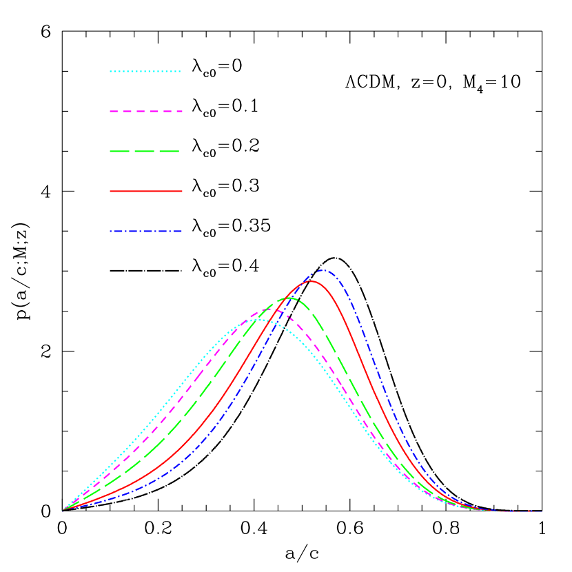
Figure 1 plots the $\lambda_{c0}$-dependence of $p(a/c;M,z)$ in the $\Lambda$CDM model: $\lambda_{c0}=0$, $0.1$, $0.2$, $0.3$, $0.35$ and $0.4$ (dotted, dashed, long-dashed, solid, dot-dashed, and dot-long-dashed lines, respectively). For this plot, we choose the halo mass $M_{4}=10$ at $z=0$ for definiteness. The axis-ratio distribution of dark halos shifts toward the high axis-ratio side (more spherical) as $\lambda_{c0}$ increases. This is theoretically understandable since higher values of $\lambda_{c0}$ correspond to those Lagrangian regions whose major axis lengths are closer to the other two (see eq.[7]). Given such, we adopt $\lambda_{c0}=0.37$ in the analysis below, following Lee & Shandarin (1998)

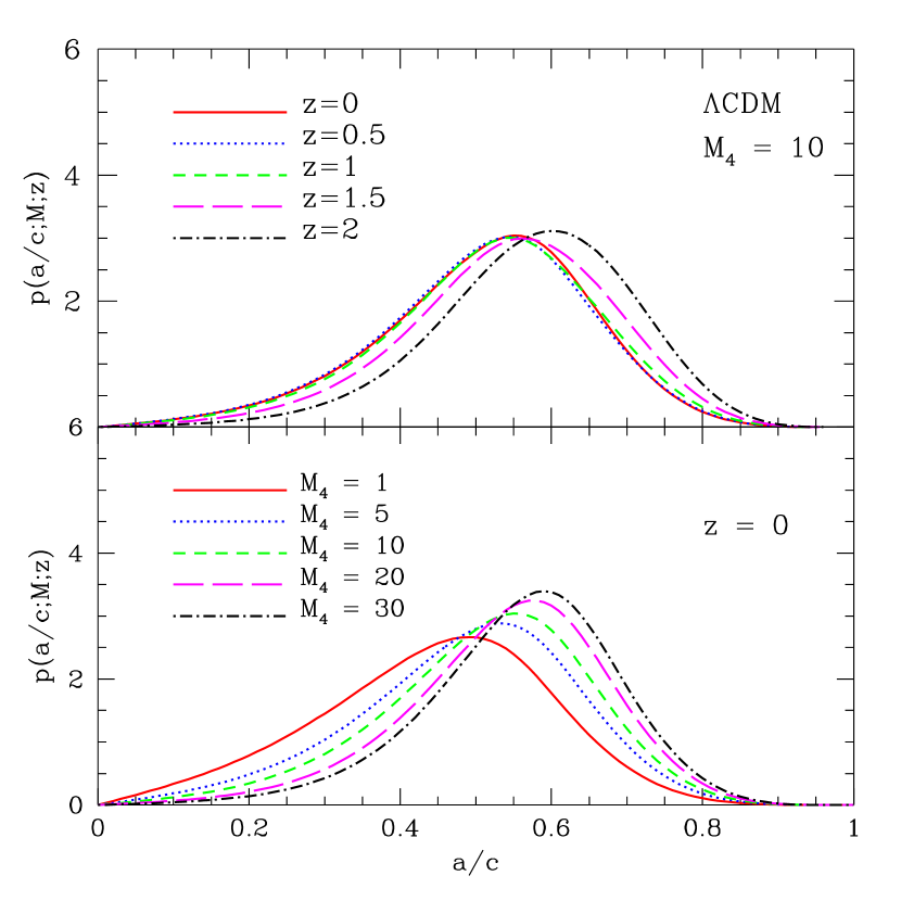
Figure 2 shows how $p(a/c;M,z)$ depends on the halo mass and the redshift for the case of $\Lambda$CDM. The upper panel shows the $z$-dependence of $p(a/c;M,z)$ for a fixed mass scale of $M_{4}=10$ at redshift $z=0$, $0.5$, $1$, $1.5$ and $2$ (solid, dotted, dashed, long-dashed, and dot-dashed) respectively. While the lower panel plots the mass-dependence of $p(a/c;M,z)$ at $z=0$ for $M_{4}=1,5,10,20$ and $30$ (solid, dotted, dashed, long-dashed, and dot-dashed) respectively. As can be seen, the analytic distribution $p(a/c;M,z)$ depends on the halo mass and redshift consistently: the distribution moves toward the high axis-ratio section as the halo mass and the redshift increase.

In other words, our analytic model predicts that the more massive a dark halos is, the less elliptical it is, and that a dark halo of given mass is less elliptical at earlier epochs. These two trends are consistent with the theoretical work of Bernardeau (1994). By applying the perturbation theory to a primordial Gaussian density field, he proved theoretically that the larger halos formed at higher density peaks are rounder. However, these trends are opposite to what is found through accurate calculations of N-body simulations: It was found in simulations that the more massive halos are more elliptical, and that the halos of given mass observed at earlier epochs are more elliptical (Bullock, 2002; Springel, White, & Hernquist, 2004; Jing & Suto, 2002; Hopkins, Bahcall, & Bode, 2004). This failure of our analytic model implies that the dependences of the axis-ratio distributions on mass and redshift are not fully determined by simply applying the Zel’dovich approximation.

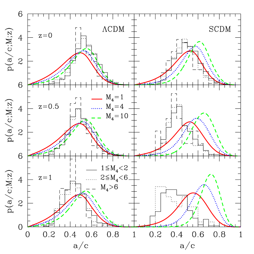
Figure 3 shows our analytic prediction (eq.[30]) at $z=0$, $0.5$, and $1$ (top, middle, and bottom, respectively) for three mass scales $M_{4}=1,4,10$ (solid, dotted, and dashed, respectively). They should be compared with the numerical results (histograms) from JS02 for the $\Lambda$CDM (left panels) and the SCDM (right panels). Clearly the analytic predictions agree with the numerical results reasonably well; they reproduce well shapes and characteristic behaviors (especially for $\Lambda$CDM) such as the peak positions, the dispersions, and the decrease of the mean axis-ratios with the increase of redshift. On the other hand, we notice that the numerical histograms slightly move toward the low axis ratio section as the halo mass increases, which disagrees with the analytical predictions. We discuss on this disagreement between the analytical and the numerical results in $\S 5$.

4 THE CONDITIONAL INTERMEDIATE-TO-MAJOR AXIS RATIO DISTRIBUTION

The probability density, $p(b/c;M;z)$, that a dark halo of mass $M$ is observed at redshift $z$ to have an intermediate-to-major axis ratio of $b/c$ can be also computed in a similar manner. However, to investigate the overall triaxiality of a dark halo, what is more relevant is the conditional probability density distribution, $p(b/c|a/c;M;z)$, that a dark halo of mass $M$ is observed at $z$ to have an intermediate-to-major axis ratio $b/c$ provided it has a minor-to-major axis ratio $a/c$. In principle, one can find this conditional probability density from the Bayes theorem:

$$p(b/c|a/c;M;z)=\frac{p(b/c,a/c;M;z)d(a/c)}{p(a/c;M;z)d(a/c)}.$$ (31)

Although it is possible to derive $p(b/c|a/c;M;z)$ analytically as well, it is not easy to construct the statistical sample either from the current simulations or from observations; there would be only a few dark halos of mass $M$ at redshift $z$ with the fixed minor-to-major $a/c$.

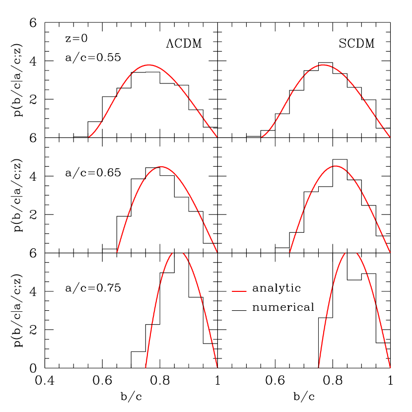
To overcome the poor number statistics, JS02 combined all the halo mass, i.e., they computed $p(b/c|a/c;z)$ instead of $p(b/c|a/c;M;z)$. For a direct comparison with their result, we compute $p(b/c|a/c;z)$ according to

$$p(b/c|a/c;z)=\int_{S_{M}}dM\int_{z}^{\infty}dz_{f}\ n(2M;z)\frac{\partial p_{f}(z_{f};2M,z)}{\partial z_{f}}\ p(b/c|a/c;2M;z_{f}),$$ (32)

where $p(b/c|a/c;2M;z_{f})$ is given as equation (18), $n(M;z)$ represents the number density of dark halos of mass $M$ that exist at $z$, and $S_{M}$ represents the whole mass range to be considered. In practice, we use the fitting formula given by Sheth & Tormen (1999) for $n(M;z)$.

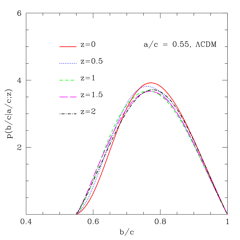
Figure 4 illustrates the redshift-dependence of $p(b/c|a/c;z)$ in the $\Lambda$CDM model at $z=0$, $0.5$, $1$, $1.5$ and $2$ (solid, dotted, dashed, long-dashed, and dot-dashed) respectively. The minor-to-major axis ratio is fixed to be $a/c=0.55$. As one can see, the conditional distribution $p(b/c|a/c;z)$ is insensitive to the redshift, which is also consistent with the finding of JS02.

Figure 5 compares the analytic predictions (curves) with the numerical findings (histograms) for $a/c=0.55$, $0.65$, and $0.75$ (top, middle, and bottom, respectively) at $z=0$ in $\Lambda$CDM (left panels) and SCDM (right panels) models. The histograms are computed by averaging over $0.5\leq a/c<0.6$, $0.6\leq a/c<0.7$, and $0.7\leq a/c<0.8$ (top, middle, and bottom, respectively). The agreement between analytic and numerical results is quite satisfactory.

5 DISCUSSIONS AND CONCLUSIONS

We have derived an analytic expression for the axis-ratio distribution of triaxial dark matter halos for the first time. In constructing the analytic model, we adopted the cosmic web picture in which the ellipticities of dark matter halos are induced by the coherent tidal fields in the initial density fluctuations, and employed the Zel’dovich-type collapse condition as a diagnostics. Our analytic model is successful in reproducing the basic behaviors on a qualitative level found from the previous numerical simulations (JS02). This ensures our basic picture that the origin of the halo triaxiality is the filamentarity of the initial density field. Nevertheless we found a discrepancy with the numerical results on a quantitative level; in particular the predicted dependences of the halo triaxiality on mass and redshift seem inconsistent with the numerical results.

In order for the future improvements, let us critically discuss possible caveats in our analytic approaches: First of all, we use a cooked-up collapse condition of $\delta=\delta_{c}$ and $\lambda_{3}\geq\lambda_{c}$. What we really mean to have is a practical and simple collapse condition for the formation of a triaxial dark halo in the nodes of filamentary web of the density field by combining the density peak formalism and the Zel’dovich approximation. This collapse condition is theoretically unjustified.

How to identify a triaxial halo and where to locate the corresponding Lagrangian site in the linear density field is a touchy issue in the non-spherical dynamical model. Although Bond & Myers (1996) proposed the peak patch picture as a complete non-spherical model, their formalism is too complicated to follow analytically in practice. Besides, as discussed in Suto (2002), there is still no unanimous agreement among theory, observations, and simulations about how to define a gravitationally bound object in practice. The disagreement among the three become more serious when a dark halo is to be described as triaxial. Hence, to find a theoretically justified criterion for the formation of a triaxial dark halo and to derive the axis-ratio distribution more rigorously with the criterion, it will be necessary to address this difficult issue first, which is beyond the scope of this paper.

As Bernardeau (1994) proved theoretically that a rare event in the linear density field is inclined to be quite spherical. In other words, a linear over-dense region of high-mass must be more spherical than a low-mass over-dense region. This is the case that our analytic distribution predicts. The difference in the trends with mass and redshift between our model and the simulation results may be caused by the fact that in reality the shape of a dark halo must be affected by subsequent nonlinear clustering process. We argue here that the nonlinear merging event must play a key role in increasing the halo ellipticity. Many N-body studies demonstrated that the merging event occurs anisotropically along filaments (e.g., West, Villumsen, & Dekel, 1991; van Haarlem & van de Weygaert, 1993; Dubinski, 1998; Faltenbacher et al., 2002). This anisotropic merging event tends to make the shapes of dark halos elongated by aligning their substructures along with the orientation of their major axes (e.g., Knebe et al., 2004). Moreover, it was also shown that the merging process is more rapid for the case of higher mass halos (Zhao et al., 2003). The tendency of being more spherical in the higher-mass section of the linear density field (Bernardeau, 1994) is likely to be compensated by the anisotropic merging effect. Therefore, the overall dependence of the axis-ratio distribution on the halo mass and redshift may be weakened by this compensating effect. Our future work is in the direction of incorporating semi-analytically the anisotropic merging process into our analytic model.

In passing, it is interesting to note that the anisotropic merging of dark halos along filaments has an implication about the mass function of dark halos. In the standard mass function theory based on the Press-Schechter theory, the mass function is independent of the power-spectrum. If the merging really occurs in an anisotropic way along filaments, however, the filamentarity in the medium must affect the final mass distribution of dark halos. For example, for the case of a power-law spectrum, the mass function might depend on the power-law index sensitively, since the filamentarity of the density field should depend on the power-law index. We wish to present the effect of anisotropic merging on the mass distribution of dark halos in the near future (Lee & Jing 2005, in preparation).

The discrepancy between our analytic model and the simulation results on the mass and redshift dependences implies that the shapes of dark halos are not fully determined by simply applying the Zel’dovich approximation. Rather, one has to take into account complicated nonlinear gravitational clustering like the anisotropic merging event. Nevertheless, the overall agreement of our analytic model with the simulation results gives us a hope that our analytic model will be useful in quantifying how the initial cosmic web induces the ellipticity of dark matter halos, and provide a first theoretical step toward the goal of using the ellipticity distribution of galaxy clusters as a new cosmological probe (Lee 2005, in preparation).

Figure 1: Probability density distribution of the axis ratio $a/c$ of halos for the five different cases of the short-axis cut-off in the $\Lambda$ CDM model; $\lambda_{c0}=0$, $0.1$, $0.2$, $0.3$, $0.35$ and $0.4$ (dotted, dashed, long-dashed, solid, dot-dashed, and dot-long dashed lines) respectively. Here, the halo mass and redshift are set to be $M_{4}\equiv M/(2.07\times 10^{13}\Omega_{m}h^{-1}M_{\odot})=10$ and $z=0$, respectively.

Figure 2: Behavior of the probability density distributions of the axis ratio $a/c$ of halos with the change of observation epochs $z_{f}$ and the halo mass $M$ in the $\Lambda$ CDM model. Top: Case in which $z=0$, $0.5$, $1$, $1.5$ and $2$ (solid, dotted, dashed, long-dashed, and dot-dashed, respectively). Bottom: Case in which $M_{4}=1$, $5$, $10$, $20$ and $30$ (solid, dotted, dashed, long-dashed, and dot-dashed,respectively), where $M_{4}\equiv M/(2.07\times 10^{13}\Omega_{m}h^{-1}M_{\odot})$.

Figure 3: Probability density distributions of the axis ratio $a/c$ of halos in the $\Lambda$ CDM (left) and SCDM (right) models at three different observation epochs; $z=0$, $0.5$,and $1$ (top, middle, and bottom panels, respectively), with the choice of $\lambda_{c0}=0.37$. In each panel, the histograms represent the numerical results (Jing & Suto, 2002) for those halos of mass; $1\leq M_{4}<2$, $2\leq M_{4}<6$, and $M_{4}\geq 6$ (thin solid, dotted, and dashed lines, respectively.) where $M_{4}\equiv M/(2.07\times 10^{13}\Omega_{m}h^{-1}M_{\odot})$, while the curves represent the analytic results (see eq.[26]) for those halos of mass; $M_{4}=1$, $M_{4}=4$, and $M_{4}=10$ (thick solid, dotted, and dashed lines), respectively.

Figure 4: Behavior of the conditional probability density distributions of the axis ratio $b/c$ at $z=0$, $0.5$, $1$, $1.5$ and $2$ (solid, dotted, dashed, long-dashed, and dot-dashed), respectively.

Figure 5: Conditional probability density distributions of the axis ratio $a/c$ of halos in the $\Lambda$ CDM (left) and SCDM (right) models provided that the minor-to-major axis ratio has a certain value: $a/c=0.55$, $0.65$ and $a/c=0.75$ (top, middle, and bottom panels), respectively at $z=0$. In each panel, the histogram and the curve represent the numerical (Jing & Suto, 2002) and the analytic results, respectively.

References

- Bailin & Steinmetz (2004) Bailin, J., & Steinmetz, M. 2004, ApJ, 616, 27
- Bardeen et al. (1986) Bardeen, J. M., Bond, J. R., Kaiser, N., & Szalay, A. S. 1986, ApJ, 304, 15
- Bernardeau (1994) Bernardeau, F. 1994, ApJ, 427, 51
- Bond & Myers (1996) Bond, J. R., & Myers, S. T. 1996, ApJ, 103, 63
- Bond, Kofman, & Pogosyan (1996) Bond, J., R., Kofman, L., & Pogosyan, D. 1996, Nature, 380, 603
- Bullock (2002) Bullock, J. S. 2002, Proceedings of the Yale Cosmology Workshop 2001, “The Shapes of Galaxies and Their Dark Matter Halos”, (Singapore: World Scientific), p.109
- Dalal, Holder, & Hennawi (2004) Dalal, N., Holder, G., & Hennawi, J. F. 2004, ApJ, 609, 50
- Doroshkevich (1970) Doroshkevich, A.G., 1970, Astrofizika, 3, 175
- Dubinski (1998) Dubinski, J. 1998, 502, 141
- Faltenbacher et al. (2002) Faltenbacher, A., Kerscher, M., Gottloeber, S., & Mueller, M. 2002, A&A, 395, 1
- Frenk et al. (1988) Frenk, C. S., White, S. D. M., Davis, M., Efstathiou, G. 1988, ApJ, 327, 507
- Hopkins, Bahcall, & Bode (2004) Hopkins, P. F., Bahcall, N., & Bode, P. 2004, preprint (atro-ph/0409652)
- Jing & Suto (2002) Jing, Y. P. & Suto, Y. 2002, ApJ, 574, 538 (JS02)
- Kasun & Evrard (2004) Kasun, S.F., Evrard, A.E. 2004, preprint, astroph/0412161
- Kitayama & Suto (1996) Kitayama, T. & Suto, Y. 1996, ApJ, 469, 480
- Knebe et al. (2004) Knebe, A. et al. 2004, ApJ, 603, 7
- Lacey & Cole (1994) Lacey, C. & Cole, S. 1994, MNRAS, 271, 676
- Lahav et al. (1991) Lahav, O., Lilje, P. B., Primack, J. R., & Rees, M. J. 1991, MNRAS, 251, 128
- Lee & Shandarin (1998) Lee, J. & Shandarin, S.F. 1998, ApJ, 500, 14
- Lee & Pen (2000) Lee, J. & Pen, U. L. 2000, ApJ, 532, 5
- Melott, Chamber, & Miller (2001) Melott, A. L., Chambers, S. W., & Miller, C. J. 2001, ApJ, 559, L75
- Moore et al. (1999) Moore, B., Quinn, T., Governato, F., Stadel, J., & Lake, G. 1999, MNRAS, 310, 1147
- Navaro, Frenk, & White (1997) Navarro, J. F., Frenk, C. S., & White, S. D. M. 1996, ApJ, 462, 563
- Oguri, Lee, & Suto (2003) Oguri, M., Lee, J., & Suto, Y. 2003, ApJ, 599, 7
- Oguri & Keeton (2004) Oguri, M., & Keeton, C. R. 2004, ApJ, 610, 663
- Peacock (1999) Peacock, J. A. 1999, Cosmological Physics, (Cambridge :Cambridge Univ. Press)
- Plionis, Barrow, & Frenck (1991) Plionis, M., Barrow, J. D., & Frenk, C. S. 1991, MNRAS, 249, 662
- Porciani, Dekel, & Hoffman (2002) Porciani, C., Dekel, A., & Hoffman, Y. 2002, MNRAS, 332, 325
- Press & Schechter (1974) Press, W., & Schechter, P. 1974, ApJ, 187, 425
- Sheth & Tormen (1999) Sheth, R., & Tormen, G. 1999, MNRAS, 308, 119
- Springel, White, & Hernquist (2004) Springel, V.; White, S. D. M.; Hernquist, L. 2004, Proceedings of the International Astronomical Union Symposium 2003, “The shapes of simulated dark matter halos”, (San Francisco: Astronomical Society of the Pacific), p.421
- Suto (2002) Suto, Y. 2002, AMiBA 2001: High-z Clusters, Missing Baryons, and CMB Polarization”, (San Francisco : A. D. P. CONF. SER.), 257, 195
- Suwa et al. (2003) Suwa, T., Habe, A., Yoshikawa, K., & Okamoto, T. 2003, ApJ, 588, 7
- van Haarlem & van de Weygaert (1993) van Haarlem, M., & van de Weygaert, R. 1993, ApJ, 418, 544
- Warren et al. (1992) Warren, M. S., Quinn, P. J., Salmon, J. K., Zurek, W. H., ApJ, 399, 405
- West (1989) West, M. J. 1989, ApJ, 347, 610
- West, Villumsen, & Dekel (1991) West, M. J., Villumsen, C., & Dekel, A. 1991, ApJ, 369, 287
- Yang, Yu, & Shen (2004) Yang, R., Yu, J., & Shen, G. P. 2004, Chinese Journal of Astronomy & Astrophysics, 4, 105
- Zhao et al. (2003) Zhao, D. H., Jing, Y. P., Mo, H. J.; Borner, G. 2003, ApJ, 597, L9
- Zeldovich (1970) Zel’dovich, Y. B. 1970, A& A, 5, 84