Ly$\mn@boldsymbol{\alpha}$ Flux Power Spectrum and Its Covariance

Abstract

We analyze the flux power spectrum and its covariance using simulated Ly$\alpha$ forests. We find that pseudo-hydro techniques are good approximations of hydrodynamical simulations at high redshift. However, the pseudo-hydro techniques fail at low redshift because they are insufficient for characterizing some components of the low-redshift intergalactic medium, notably the warm-hot intergalactic medium. Hence, to use the low-redshift Ly$\alpha$ flux power spectrum to constrain cosmology, one would need realistic hydrodynamical simulations. By comparing (one-dimensional) mass statistics with flux statistics, we show that the nonlinear transform between density and flux quenches the fluctuations so that the flux power spectrum is much less sensitive to cosmological parameters than the one-dimensional mass power spectrum. The covariance of the flux power spectrum is nearly Gaussian. As such, the uncertainties of the underlying mass power spectrum could still be large, even though the flux power spectrum can be precisely determined from a small number of lines of sight.

1 Introduction

The Ly$\alpha$ forest is a useful tool for studying the cosmic density field over a wide range of redshift that has not been easily accessible to other types of observations. For each line of sight (LOS) to a quasar, one can sample the density field almost continuously in one dimension. With enough LOSs covering up to $z\sim 6$, the Ly$\alpha$ forest will enable us to establish a more complete picture of the universe and its evolution, and, subsequently, to determine cosmological parameters.

Statistics of the Ly$\alpha$ forest have been applied to many aspects of large-scale structure studies such as recovering the initial linear mass power spectrum (PS; Croft et al., 1998, 1999; Hui, 1999; Feng & Fang, 2000; McDonald et al., 2000, 2004b; Croft et al., 2002; Gnedin & Hamilton, 2002; Zaldarriaga, Scoccimarro & Hui, 2003), measuring the flux PS and bispectrum (Hui et al., 2001; Mandelbaum et al., 2003; Kim et al., 2004; Viel et al., 2004), estimating cosmological parameters (McDonald & Miralda-Escudé, 1999; Zaldarriaga, Hui & Tegmark, 2001; Croft et al., 2002; McDonald, 2003; Seljak, McDonald & Makarov, 2003; Viel et al., 2003; Seljak et al., 2004; Viel, Weller & Haehnelt, 2004; Lidz et al., 2005), inverting the Ly$\alpha$ forest (Nusser & Haehnelt, 1999; Pichon et al., 2001; Zhan, 2003), finding the applicable range of the hierarchical clustering model (Feng, Pando & Fang, 2001; Zhan, Jamkhedkar & Fang, 2001), and estimating the velocity field (Zhan & Fang, 2002). These studies show that the Ly$\alpha$ forest has provided an important complement to studies based on galaxy and QSO samples.

In fact, the Ly$\alpha$ forest is becoming a major player in precision cosmology. It is one of the three measures (others being the cosmic microwave background and galaxy redshift surveys) in Spergel et al. (2003) that show a tantalizing hint of a possible running spectral index, which could have a significant impact on inflationary models. However, the degeneracy between the amplitude and slope of the flux PS that has arisen owing to uncertainties in the mean transmission weakens the argument for a running spectral index (Seljak, McDonald & Makarov, 2003). This motivates us to pursue a better understanding of the uncertainties in the Ly$\alpha$ flux statistics in the era of precision cosmology.

A number of authors have examined the effects of metal lines, continuum fitting, strong discrete absorptions systems, damping wings, ionizing radiation fluctuations, galactic winds, and simulation details (Hui et al., 2001; Viel et al., 2004; Meiksin & White, 2004; McDonald et al., 2004a, b). In this paper, we focus on the following facets of the Ly$\alpha$ forest. Firstly, we evaluate the performance of pseudo-hydro techniques (e.g. Petitjean, Mücket & Kates, 1995; Croft et al., 1998) by comparing their results to those from full hydrodynamical simulations and by varying pseudo-hydro parameters. We show that a systematic difference between pseudo-hydro and full-hydro results exists, which might cause a bias in cosmological parameter estimation. Thus, careful calibrations of pseudo-hydro techniques over a large dynamic range are necessary for precision cosmology.

Secondly, the Ly$\alpha$ flux is a nonlinear transform of the one-dimensional density field. Fluctuations in the flux and the sample variance of the flux PS are much smaller than those of the density field. Consequently, one can measure the flux PS to a high precision with a small number of LOSs, but to achieve the same precision in the mass PS one needs a lot more LOSs.

Thirdly, the Ly$\alpha$ flux is nearly Gaussian, while the one-dimensional density field exhibits stark non-Gaussianity (Zhan & Eisenstein, 2005). These are not characterized by the PS but by higher-order statistics such as the covariance of the PS. We quantify the correlation between Fourier modes in both flux and density fields using the covariance of the PS.

Finally, we point out the difficulty with extending the Ly$\alpha$ flux PS analysis to low redshift. Since the non-Gaussianity of the density field becomes stronger at lower redshift, one would need even more LOSs to recover the one-dimensional mass PS at the same precision that one would at high redshift. Meanwhile, pseudo-hydro techniques work poorly at low redshift so that one would have to utilize more time-consuming full-hydro simulations.

The rest of the paper is organized as follows. §2 briefly describes the simulations used for the investigation. The flux PS and its covariance are illustrated in §3 and contrasted with one-dimensional mass PS and its covariance. Comparisons of flux PSs in different cosmological models are given in §4, and §5 concludes the paper. Note that in our terms the flux PS is always the one-dimensional PS of the flux $F$, not $F/\bar{F}$.

2 Simulated Ly$\mn@boldsymbol{\alpha}$ Forests

The Ly$\alpha$ forest probes deeply into the nonlinear regime of the cosmic density field. This has made numerical simulations indispensable for understanding the nature of the Ly$\alpha$ forest and inferring cosmological parameters from flux statistics. Two types of cosmological simulations have been commonly used to simulate the Ly$\alpha$ forest. One is pure cold dark matter (CDM), or $N$-body simulations, which assume that baryons trace the dark matter (e.g. Petitjean, Mücket & Kates, 1995; Croft et al., 1998; Riediger, Petitjean & Mücket, 1998). The other is hydrodynamical simulations (e.g. Cen et al., 1994; Zhang, Anninos & Norman, 1995; Hernquist et al., 1996; Davé et al., 1997). Although full hydrodynamical simulations are well suited for studies of the Ly$\alpha$ forest, they are currently too time-consuming to explore a large cosmological parameter space as one often desires. Whereas, $N$-body simulations run much faster, and hence can be used to cover a wider range of cosmological models in a practical time. Other types of simulations such as hydro-particle-mesh simulations (HPM, Gnedin & Hui, 1998) and the simple log-normal model (Bi & Davidsen, 1997) have also been used to study the Ly$\alpha$ forest.

2.1 Hydrodynamical Simulations with Photoionization

We use a hydrodynamical simulation (HLCDM) for this study. It is a variant of the low-density-and-flat CDM (LCDM) model with a slight tilt of the initial power spectral index $n$ (see Table 1). HLCDM evolves $128^{3}$ CDM particles and $128^{3}$ gas particles from $z=49$ to 0 using Parallel TreeSPH (Davé, Dubinski & Hernquist, 1997). The box size is 22.222 $h^{-1}$Mpc in each dimension with a 5 $h^{-1}$ kpc resolution. The simulation also includes star formation with feedback and photoionization (Katz, Weinberg & Hernquist, 1996). The UV ionization background is from Haardt & Madau (1996).

We simplify the method in the software tool, tipsy, to produce Ly$\alpha$ forests. The procedures are outlined below. For convenience, we assume zero metallicity and do not include noise.

Snapshots of the simulations contain the position ${\bf r}_{i}$ and velocity ${\bf v}_{i}$ of each particle, where $i$ labels the $i$th particle. Smooth-particle hydrodynamics (SPH) defines the baryon density $\rho_{\rm b}({\bf x})$ at any location to be a sum of contributions from all nearby gas particles, i.e.

$$\rho_{\rm b}({\bf x})=\sum_{i=1}^{N_{\rm p}}m_{i}\,w(|{\bf x}-{\bf r}_{i}|,\epsilon^{j}_{i}),$$ (1)

where $N_{\rm p}$ is the total number of particles, $w$ is the density kernel or the assignment function, $m_{i}$ is the mass of particle $i$, and $\epsilon^{j}_{i}$ is the smoothing length determined by the distance between particle $i$ and its $j$th neighbor ($j=32$ in this paper). In practice, densities are assigned on a discrete grid for further analysis. We employ a spherically symmetric spline kernel from Monaghan & Lattanzio (1985), which is also used in TreeSPH for force calculations. It has the form

$$w(r,\epsilon)=\frac{1}{\pi\epsilon^{3}}\left\{\begin{array}[]{ll}1-\frac{3}{2}\left(\frac{r}{\epsilon}\right)^{2}+\frac{3}{4}\left(\frac{r}{\epsilon}\right)^{3}&\quad 0\leq r<\epsilon\\ \frac{1}{4}\left[2-\frac{r}{\epsilon}\right]^{3}&\quad\epsilon\leq r<2\epsilon\\ 0&\quad r\geq 2\epsilon,\\ \end{array}\right.$$ (2)

which vanishes beyond the radius $2\epsilon$ and has a smooth gradient everywhere. This density kernel is an effective low-pass filter that suppresses fluctuations on scales smaller than $2\epsilon$ ($k>\pi/\epsilon$).

For each gas particle we assume a universal hydrogen fraction of $0.76$ to convert the baryon density to hydrogen density, and calculate the ionization equilibrium Hi density at the particle temperature. In principle, LOSs may be sampled in any random direction, but for computational simplicity we assign the Hi density on a grid of $256^{3}$ nodes, and then extract one-dimensional fields randomly from this grid. We have tried a higher-resolution grid of $512^{3}$ nodes, and the results are not affected on scales above $0.6$ $h^{-1}$Mpc ($k<10$ $h$ Mpc^-1). Node temperatures and velocities are also assigned as weighted averages of contributing particles. The weight is proportional to the Hi mass contribution of each particle.

The assumption of ionization equilibrium certainly breaks down in very dynamic regions such as shocks. However, since the equilibrium Hi fraction calculated in such regions is already considerably lower than elsewhere, there will not be much of an effect on simulated Ly$\alpha$ forests, even if additional shock physics can further reduce the Hi fraction by orders of magnitude. In addition, shock fronts, unlike shocked gas, only occupy a small fraction of the total simulation volume, so they could not have too much impact on the Ly$\alpha$ forest.

Table 1: Parameters of the simulations.

Model	Type	$\Omega$	$\Omega_{\rm b}$	$\Omega_{\Lambda}$	$h$	$n$	$\sigma_{\mathrm{8}}$
HLCDM	Hydro.	0.4	0.05	0.6	0.65	0.95	0.8
TCDM	$N$-Body	0.3	0.04	0.7	0.7	1.1	0.8
LCDM1	$N$-Body	0.3	0.04	0.7	0.7	1.0	0.8
LCDM2	$N$-Body	0.3	0.04	0.7	0.7	1.0	1.0
OCDM	$N$-Body	0.3	0.04	0	0.7	1.0	0.8

With the exception of HLCDM, the baryon density is used only for generating the initial mass PS.

With the Hi density along the LOS, one can determine the Ly$\alpha$ optical depth $\tau$ and transmitted Ly$\alpha$ flux $F$ of each pixel (each node of the density grid). The mean flux $\bar{F}$ of the Ly$\alpha$ forest is constrained by observations. We adjust the intensity of the UV ionization background $\Gamma_{\rm UV}$ so that the mean flux of all pixels in the simulations follows

$$\bar{F}(z)\simeq\left\{\begin{array}[]{ll}\exp\left[-0.0032\,(1+z)^{3.37\pm 0.2}\right]&\ \ 1.5\leq z\leq 4\\ 0.97-0.025\,z\pm(0.003+0.005\,z)&\ \ 0\leq z<1.5.\\ \end{array}\right.$$ (3)

The high-redshift part of the mean flux formula is given by the observations of Kim et al. (2002), which is consistent with others (Lu et al., 1996; Rauch et al., 1997; McDonald et al., 2000). Since the mean opacity of the low-redshift Ly$\alpha$ forest is somewhat uncertain (Penton, Stocke and Shull, 2004), we take the simulated mean flux from Davé et al. (1999) as the fiducial mean flux at low redshift. Thermal broadening is added afterward using the temperature of each pixel. Note that thermal broadening smoothes out small-scale fluctuations in the Ly$\alpha$ forest without altering the mean flux very much. Therefore, it preferentially reduces the flux power on small scales.

There is a slight inconsistency in that HLCDM has already included the UV ionization background, yet we need to adjust the intensity of the UV radiation on outputs of the simulation to fit the mean flux. This inconsistency does not significantly affect the results that follow because the temperature of the intergalactic medium (IGM) is not sensitive to the UV background intensity (Croft et al., 1997). In fact, the simulation outputs are able to reproduce the observed mean flux with their internal UV ionization background (Davé et al., 1999). External adjustments are only needed to vary the mean flux within the given observational and numerical uncertainties. Thus, even if the intensities of the externally adjusted UV background were used internally in the simulations, the LOS Ly$\alpha$ absorption would not change appreciably.

Table 2: Methods for generating the Ly$\alpha$ forest.

Method	Particle	$\rho_{\rm b}$	$T_{\rm node}$	$\tau$
HYDRO	SPH		SPH	Ion. Eq.
BA-TE-IE	SPH		Thermal Eq.	Ion. Eq.
DM-TE-IE	CDM	$\propto\rho_{\rm d}$	Thermal Eq.	Ion. Eq.
DM-EOS	CDM	$\propto\rho_{\rm d}$	$T_{0}(\rho_{\rm b}/\bar{\rho}_{\rm b})^{\gamma-1}$	$\propto(\rho_{\rm b}/\bar{\rho}_{\rm b})^{\beta}$

2.2 Pseudo-Hydro Techniques

Petitjean, Mücket & Kates (1995) developed a pseudo-hydro technique for generating Ly$\alpha$ forests from $N$-body simulations. They assume that the baryons trace the dark matter and calculate the optical depths of baryons assuming ionization equilibrium. We further simplify their method by also assuming thermal equilibrium (labelled as DM-TE-IE in Table 2).

Separately, Croft et al. (1998) proposed a slightly different pseudo-hydro technique (labelled as DM-EOS). In addition to assuming baryons to trace dark matter, they also make use of the fact that, in thermal equilibrium, the equation of state (EOS) of the IGM gives rise to an approximate temperature–density relation

$$T=T_{0}(\rho_{\rm b}/\bar{\rho}_{\rm b})^{\gamma-1},$$ (4)

where $T_{0}\sim 10^{4}$ K, $1.3\leq\gamma\leq 1.6$, and $\rho_{\rm b}/\bar{\rho}_{\rm b}\la 10$ (Hui & Gnedin, 1997). Since the Ly$\alpha$ optical depth is proportional to $\rho_{\rm b}^{2}\,T^{-0.7}$ in regions around the mean density, one finds

$$F\simeq e^{-A(\rho_{\rm b}/\bar{\rho}_{\rm b})^{\beta}}\simeq e^{-A(\rho_{\rm d}/\bar{\rho}_{\rm d})^{\beta}},$$ (5)

where $A\propto\Omega_{\rm b}^{2}\,\Gamma_{\rm UV}^{-1}T_{0}^{-0.7}$, $\beta=2.7-0.7\gamma$, and $\rho_{\rm d}$ is the dark matter density. The constant $A$ is often left as a fitting parameter adjusted to reproduce the observed mean flux.

Figure 1: Transmitted Ly$\alpha$ flux based on baryon and dark matter distributions at $z=0$. The three panels compare Ly$\alpha$ forests generated from the same LOS with methods HYDRO, BA-TE-IE, DM-TE-IE, and DM-EOS. All four methods are required to reproduce the same mean flux of $0.97$.

For comparison, we devise another method for generating Ly$\alpha$ forests from hydrodynamical simulations, in which the temperature of the gas particle is calculated assuming that the baryons are in thermal equilibrium, i.e. we discard the actual particle temperature from the simulations. We refer to this method as BA-TE-IE, and the name HYDRO is given to the full-hydrodynamical approach described in Section 2.1. One can assess the importance of shocked gas by comparing the method HYDRO with BA-TE-IE, while the difference between methods BA-TE-IE and DM-TE-IE must arise from differences in the baryon and dark matter distributions. The four methods are summarized in Table 2.

2.3 Comparison

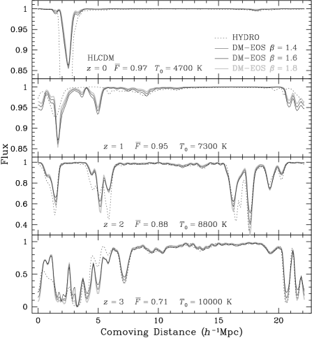
To give a visual impression of pseudo-hydro techniques, in Figures 1 and 2 we present Ly$\alpha$ forests obtained along the same LOS using the four methods, HYDRO, BA-TE-IE, DM-TE-IE, and DM-EOS. We require that the mean flux over all $256^{2}$ Ly$\alpha$ forests in all four methods match the mean flux of $0.97$ at $z=0$ and $0.71$ at $z=3$, but the mean flux of a single LOS is not necessarily the same across the methods. Since neither a simple EOS nor thermal equilibrium takes into account the substantial amount of warm-hot intergalactic medium (WHIM, Davé et al., 1999; Davé & Tripp, 2001; Davé et al., 2001) at $z=0$, pseudo-hydro techniques are expected to be less accurate at lower redshift. This is seen in Figure 1. Conversely, at $z=3$ methods HYDRO and BA-TE-IE generate nearly identical Ly$\alpha$ forests, and the difference between the Ly$\alpha$ forests generated from baryons and those from dark matter is also small.

Figure 2: The same as Fig. 1, except that the Ly$\alpha$ forests are generated from baryon and dark matter distributions at $z=3$ and the mean flux is $0.71$.

Figure 3: Flux PSs of Ly$\alpha$ forests at $z=0$, 1, 2, and 3. The Ly$\alpha$ forests are produced using the four methods listed in Table 2. Grey bands represent standard deviations of flux PSs of Ly$\alpha$ forests generated using the method HYDRO. The standard deviations are calculated among 1000 groups, each of which consists of 64 LOSs. Additional flux PSs (dash-dotted lines) are calculated using the method DM-EOS with $T_{0}=15000$ K for $z=1$, 2, and 3. Note that the flux PSs are plotted in dimensionless form, i.e. $kP_{\rm F}(k)/\pi$.

Figure 4: Fractional errors in the flux PS. The legends are the same as in Fig. 3.

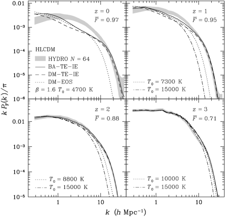
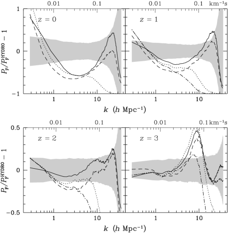
Figure 3 evaluates the statistical performance of pseudo-hydro techniques using flux PSs, and the fractional errors relative to the method HYDRO are shown in Figure 4. The grey bands are the standard deviations of the flux PSs for Ly$\alpha$ forests produced using the method HYDRO. The standard deviations are calculated among 1000 groups, each of which contains 64 LOSs randomly selected with no repetition. The total length of 64 LOSs is 180000 km s^-1 at $z=3$, about 10% less than the corresponding low resolution sample in Croft et al. (2002). There is a good agreement among all methods at $z=3$ for $k$ less than a few $h$ Mpc^-1 with a less-than-10% difference in the slopes of the flux PS. Whereas, all the three pseudo-hydro methods, BA-TE-IE (solid lines), DM-TE-IE (dashed lines), and DM-EOS (dotted lines) fail to converge on HYDRO (grey bands) at $z=0$ owing to the WHIM. In fact, methods HYDRO and BA-TE-IE have identical baryon distributions, so that the difference in their flux PSs can only be attributed to the IGM temperature, which is greatly affected by shock heating at low redshift. Hence, one can conclude that the temperature structure of the IGM is critical to the low-redshift Ly$\alpha$ forest and flux PS. Furthermore, the sensitivity of the low-redshift Ly$\alpha$ forest to hydrodynamical effects forewarns us of the importance of other astrophysical effects, which could make the low-redshift Ly$\alpha$ forest an ideal test for realistic hydrodynamical simulations.

The mean-density temperature of the IGM, $T_{0}$, does not alter the optical depth in the method DM-EOS because it is absorbed into the constant $A$ in the approximation $F=\exp\left[-A(\rho/\bar{\rho})^{\beta}\right]$, which is adjusted to fit the observed mean flux. However, $T_{0}$ can affect simulated Ly$\alpha$ forests through thermal broadening as indicated by the fast drop at large $k$ of the flux PSs for the method DM-EOS. To test this, We reproduce Ly$\alpha$ forests at $z=1$, 2, and 3 using $T_{0}=15000$ K, which is 1.5 to 2 times the mean-density temperature of the IGM in HLCDM. Flux PSs of these Ly$\alpha$ forests are shown in dash-dotted lines in Figures 3 and 4. One sees that the higher mean-density temperature reduces more flux power on small scales while leaving flux PSs unchanged on large scales.

The poor performance of the pseudo-hydro techniques at low redshift means that there will be a substantial systematic error in the recovered one-dimensional linear mass PS if it is obtained by applying the pseudo-hydro ratio between the one-dimensional linear mass PS and flux PS to the observed low-redshift flux PS. For example, at $z=2$ the slope of the flux PS of the method DM-EOS differ from that of HYDRO by 32% to -19% (rms 17%) within $0.3\ \mbox{$h$ Mpc${}^{-1}$}<k<2\ \mbox{$h$ Mpc${}^{-1}$}$, yet both flux PSs have the same underlying one-dimensional linear mass PS. Thus, the DM-EOS method will recover a one-dimensional mass PS that is 32% to -19% off compared to HYDRO. Since the slope of the one-dimensional mass PS determines the shape of the three-dimensional mass PS (the amplitude has to be calibrated separately), the error in the slope will give rise to an error in the shape of the recovered three-dimensional linear mass PS.

Figure 5: Left panel: The neutral hydrogen number density $n_{\rm HI}$ as a function of the baryon density contrast $\rho_{\rm b}/\bar{\rho}_{\rm b}$. The grey dots correspond to the values of $2.5\%$ gas particles in the simulation HLCDM that are calculated using the method HYDRO, and the solid line is given by thermal equilibrium and ionization equilibrium, i.e. the method BA-TE-IE. From top to bottom, the three horizontal dashed lines mark the Hi number densities that would give rise to a pixel flux level of 0.01, 0.71 (the mean flux at $z=3$), and 0.99, if the Hi number densities were Hi number densities of the node. Right panel: Fractional error in the flux PS. The grey band represents the standard deviation of the flux PS of Ly$\alpha$ forests generated using the method HYDRO as in Fig. 3, and the lines are flux PSs of Ly$\alpha$ forests generated using the method BA-TE-IE (solid line), BA-TE-IE for $\rho_{\rm b}/\bar{\rho}_{\rm b}>1$ and HYDRO for $\rho_{\rm b}/\bar{\rho}_{\rm b}\leq 1$ (dashed line), and HYDRO for $\rho_{\rm b}/\bar{\rho}_{\rm b}>1$ and BA-TE-IE for $\rho_{\rm b}/\bar{\rho}_{\rm b}\leq 1$ (dotted line).

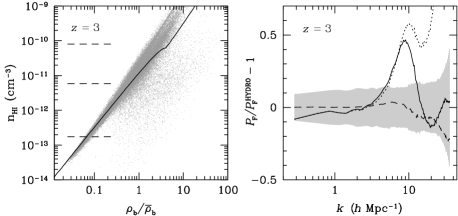
Pseudo-hydro techniques replace the complex distribution of the neutral hydrogen number density $n_{\rm HI}$ at a given baryon density contrast $\rho_{\rm b}/\bar{\rho_{\rm b}}$ with a single function (see the left panel of Figure 5). This approximation has two effects: 1) it decreases (increases) the optical depth of some particles and depresses (amplifies) flux fluctuations, and 2) it reduces the scatter in the optical depth at a given density and smoothes the flux. The former is more important at low densities where pseudo-hydro techniques tend to overestimate the optical depth, while the latter is more important at high densities. This is supported by Figure 2, in which pseudo-hydro fluxes display richer structures and deeper absorptions than the full-hydro flux in regions above the mean flux.

Figure 6: Ly$\alpha$ forests generated from dark matter distributions with different EOSs. The Ly$\alpha$ forests are produced from dark matter densities using $F=\exp[-A(\rho/\bar{\rho})^{\beta}]$, where $A$ is adjusted to fit the mean flux $\bar{F}$. Thermal broadening is included with temperature given by $T=T_{0}(\rho/\bar{\rho})^{\gamma-1}$.

Around $k=10$ $h$ Mpc^-1, there is a relative increase of the flux PS from methods BA-TE-IE and DM-TE-IE with respect to that from HYDRO in all the redshift panels in Figure 4. This appears to be the result of the competition between the increase of the optical depth at low densities and the reduction of the scatter of the optical depth at high densities in the pseudo-hydro methods. The flux PS from the method DM-EOS shares the same characteristics at $z=3$, but stronger thermal broadening at lower redshift wipes out the irregularity on small scales.

To try to isolate whether it is the low or high density regions that are responsible for the discrepancies in the pseudo-hydro flux PS, we consider what happens when one applies pseudo-hydro to one density regime and full hydro the rest. We show in the right panel of Figure 5 the fractional error in the flux PS obtained by applying the method HYDRO to $\rho_{\rm b}/\bar{\rho_{\rm b}}\leq 1$ particles and BA-TE-IE to $\rho_{\rm b}/\bar{\rho_{\rm b}}>1$ particles (dashed line). With such a combination, the small-scale flux fluctuations are suppressed because full hydro produces shallower absorptions in low density regions and because pseudo-hydro eliminates those fluctuations that arise from the scatter of the optical depth in high density regions. Conversely, the opposite combination (dotted line) results in a boost of the flux PS on small scales. It is also interesting to note that the large-scale flux PS ($k<2$ $h$ Mpc^-1) is determined by the method that is applied to the low-density particles. Hence, Figure 5 suggests that the low-density particles and their treatment carry a considerable weight in the Ly$\alpha$ flux PS on all scales.

2.4 Tuning the Equation of State

The equation of state (EOS) maps density fluctuations to flux fluctuations by relating optical depths to densities. For a given density and mean flux, different EOSs will assign different optical depths, which will then alter the amplitude of the flux fluctuations and, therefore, the flux PS.

Figure 7: Flux PSs of Ly$\alpha$ forests generated from dark-matter-converted baryon densities using different EOSs. Grey bands represent standard deviations of the flux PSs of Ly$\alpha$ forests generated using the method HYDRO as in Fig. 3. Also as in Fig. 3 dimensionless PSs are plotted.

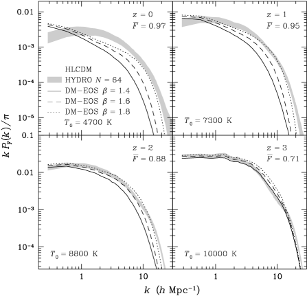
For a stiffer EOS, i.e. a smaller value of $\beta$ (larger $\gamma$), high-density regions have to absorb less Ly$\alpha$ flux, while, in compensation, low-density regions have to absorb more flux. In terms of flux, a stiff EOS leads to higher fluxes in deep (or large-equivalent-width) absorptions and lower fluxes in shallow absorptions than a soft EOS. This expectation is confirmed in Figure 6, where Ly$\alpha$ forests generated using the method DM-EOS are compared with those using the method HYDRO at $z=0$, 1, 2, and 3. The mean flux is kept the same for both methods at each epoch, varying only the EOS. The value of $\beta=1.4$ in the figures corresponds to a very stiff EOS, i.e. $\gamma=1.86$, and it is provided only for the purpose of comparison.

Figure 6 shows that low-amplitude and small-scale fluctuations in the flux are likely to be suppressed by the method DM-EOS. This reduces the flux PS on small scales as seen in Figures 3 and 4. The method DM-EOS is not a good approximation at low redshift, but it improves as redshift increases.

Since the amplitude of flux fluctuations increases with $\beta$ in Figure 6, a smaller value of $\beta$ must lead to a lower flux PS. This is observed in Figure 7, where flux PSs of Ly$\alpha$ forests obtained using the method DM-EOS with different EOSs are compared with those using the method HYDRO. Figure 7 demonstrates that one cannot tune the EOS to make the pseudo-hydro method DM-EOS work at low redshift. Again, the method DM-EOS appears to be a reasonable approximation for studies of the flux PS at $z=3$, although it may not be true for higher-order statistics. The difference among different EOSs is also less pronounced at $z=3$ because the dynamic range of the density contrast, $\rho/\bar{\rho}$, is much smaller.

3 Mass Statistics vs. Flux Statistics

3.1 Power Spectrum

The Ly$\alpha$ forest has been used to infer the linear mass PS of the cosmic density field. The nonlinear transform of the density to the flux has made it difficult to derive the (linear) mass PS from the flux PS analytically. One way to circumvent this difficulty is to use simulations to map the flux PS to the linear mass PS (e.g. Croft et al., 2002). Although the flux PS resembles the linear one-dimensional mass PS, the underlying nonlinear density field is what produces the Ly$\alpha$ forest. As such, it is important to compare the flux PS with the mass PS.

Figure 8: Flux PSs of simulated Ly$\alpha$ forests and one-dimensional mass PSs of the underlying density fields at $z=0$ and 3. The Ly$\alpha$ forests are produced with methods HYDRO and DM-TE-IE from baryon and dark matter distributions, respectively.

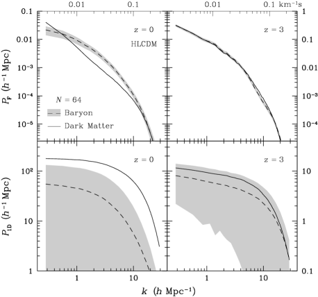
Plotted in Figure 8 are flux PSs produced using methods HYDRO and DM-TE-IE along with one-dimensional mass PSs of baryons and dark matter. The standard deviations of baryon flux PSs and mass PSs are shown in grey bands. The most prominent feature is that one-dimensional mass PSs have much larger dispersions than flux PSs. As discussed in Zhan & Eisenstein (2005), the variance in the one-dimensional mass PS is severely inflated by the trispectrum of the cosmic density field because of the non-Gaussianity.

An interesting observation is that unlike the mass PS the flux PS decreases with time. This is due to the thinning of the Ly$\alpha$ forest and the higher mean flux toward lower redshift that reduce fluctuations in the Ly$\alpha$ flux.

The nonlinear transform between baryon density and flux greatly suppresses the fluctuations. For example, the overdensity $\delta$ may vary from -1 to hundreds (tens) at $z=0$ ($z=3$), but the flux can only be between 0 and 1. With a mean flux on the order of unity, fluctuations in the flux are $10$ to $10^{2}$ times smaller than those in the cosmic density field. Hence, the flux PS is a factor of $10^{2}$ ($z=3$) to $10^{4}$ ($z=0$) times lower than the one-dimensional mass PS. Moreover, the non-Gaussianity in the cosmic density field is also strongly suppressed in the flux. Thus, the flux trispectrum is much closer to zero as compared to the mass trispectrum of the cosmic density field, and the variance of the flux PS becomes much smaller than the variance of the one-dimensional mass PS.

The near-Gaussian Ly$\alpha$ flux is probably the reason that many simulations and techniques are able to reproduce lower-order statistics of the observed Ly$\alpha$ forest, especially at high redshift. Figure 8 points out a possible problem that can arise: one could produce Ly$\alpha$ forests from wildly different density fields but still have almost identical flux PSs. For example, even though baryons and dark matter differ considerably in terms of mass PS (see also Figures 14 and 15), they are not so distinguished from each other in flux PSs at $z\geq 2$. Conversely, we are able to measure the flux PS extremely well, but the underlying mass PS may still be much less constrained.

3.2 Covariance

The covariance of the PS is a fourth-order statistic that measures the uncertainties in the PS as well as the correlation between modes. Here, we use it to explore the difference between Ly$\alpha$ forests generated using the full-hydro method HYDRO and those using the pseudo-hydro method DM-TE-IE.

Figure 9: Covariances of one-dimensional baryon and dark matter PSs at $z=0$. The upper panels are reduced covariances $\hat{C}(k,k^{\prime})$ in a linear grey scale with black being $1.2$ and white less than or equal to 0. The lower panels are cross sections of normalized covariances $C(k,k^{\prime})$ along $Q=(k+k^{\prime})/\mbox{$h^{-1}$Mpc}$. The covariances $C(k,k^{\prime})$ are multiplied by 64 for better comparison with that of GRFs, which follows $64\,C(k,k^{\prime})=\delta^{\rm K}_{n,n^{\prime}}$. All the covariances are calculated from 1000 groups, each of which consists of 64 LOSs ($N=64$) randomly selected from the density grid of HLCDM.

Figure 10: The same as Fig. 9, but for flux PSs of Ly$\alpha$ forests generated from baryons and dark matter using methods HYDRO and DM-TE-IE, respectively.

Figure 11: The same as Fig. 9, but for the simulation HLCDM at $z=3$.

Figure 12: The same as Fig. 11, but for flux PSs.

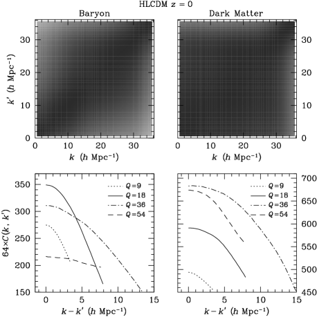
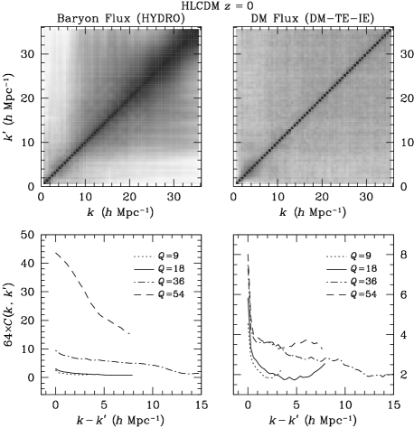
The covariance of the one-dimensional mass PS is defined as

$$\sigma^{2}_{\rm 1D}(k,k^{\prime})=\langle[P_{\rm 1D}(k)-\langle P_{\rm 1D}(k)\rangle][P_{\rm 1D}(k^{\prime})-\langle P_{\rm 1D}(k^{\prime})\rangle]\rangle,$$ (6)

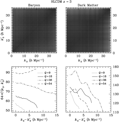
where $\langle\ldots\rangle$ stands for an ensemble average, and $P_{\rm 1D}(k)$ can be replaced by $P_{\rm F}(k)$ for the flux PS covariance $\sigma^{2}_{\rm F}(k,k^{\prime})$. Since we use a discrete Fourier transform for the analysis, the wavenumber $k$ is discrete, i.e. $k=2n\pi/L$, where $n$ assumes integer values and $L$ is the length of the spectrum. We use $k$ and $n$ interchangeably.

There is a hidden variable $N$, the number of LOSs that are averaged over to obtain the one-dimensional PS, in equation (6). For Gaussian random fields (GRFs), one can show that

$$\sigma^{2}_{\rm 1D}(k,k^{\prime})\simeq\frac{1}{N}P_{\rm 1D}^{2}(k)\,\delta^{\rm K}_{n,n^{\prime}},$$ (7)

where $\delta^{\rm K}_{n,n^{\prime}}$ is the Kronecker delta function. This also applies to the flux PS covariance. Equation (7) is only approximate owing to both the finite length of the LOSs and the correlation between the LOSs (Zhan & Eisenstein, 2005).

We also introduce the normalized covariance

$$C(k,k^{\prime})=\sigma^{2}_{\rm 1D}(k,k^{\prime})[P_{\rm 1D}(k)P_{\rm 1D}(k^{\prime})]^{-1},$$ (8)

and the reduced covariance

$$\hat{C}(k,k^{\prime})=C(k,k^{\prime})[C(k,k)C(k^{\prime},k^{\prime})]^{-1/2}.$$ (9)

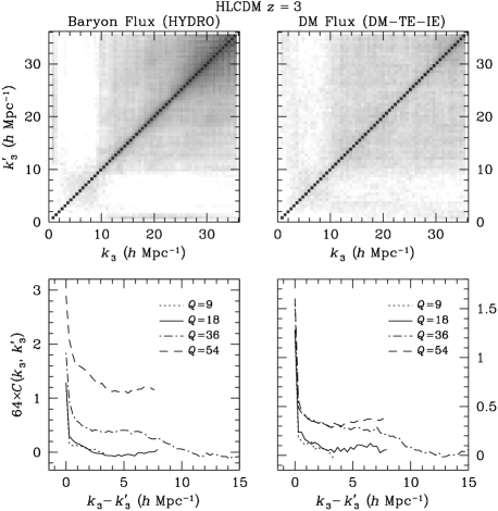
Again, $P_{\rm 1D}(k)$ can be replaced by $P_{\rm F}(k)$ for the flux PS covariance. For GRFs, both the covariance matrices are diagonal. In addition, we have $NC(k,k)=1$. The advantage of $\hat{C}(k,k^{\prime})$ is that $\hat{C}(k,k)=1$ for all fields, so that they can be compared with each other in a single grey scale.

Figures 9 and 10 illustrate the covariances $\hat{C}(k,k^{\prime})$ and $C(k,k^{\prime})$ of one-dimensional mass PSs and flux PSs at $z=0$. The covariances are calculated from 1000 groups, each of which consists of 64 LOSs ($N=64$) randomly selected from the density grid of HLCDM. For GRFs, the covariance matrix $\hat{C}(k,k^{\prime})$ is diagonal, and the normalized variance $C(k,k)$ equals $N^{-1}$. For better comparison, the covariances $C(k,k^{\prime})$ are multiplied by $N$, so that the Gaussian case has $N\,C(k,k^{\prime})=\delta^{\rm K}_{n,n^{\prime}}$. As already seen in Zhan & Eisenstein (2005), the covariances of one-dimensional mass PSs are starkly non-Gaussian. The variances in the one-dimensional mass PS are two orders of magnitude higher than expected for GRFs. The covariances of baryons are roughly a factor of 2 lower than those of dark matter. This is likely due to the pressure experienced by the SPH particles. The covariances of flux PSs have a dominant diagonal, though they are still not Gaussian. The method HYDRO gives rise to stronger correlations between high-$k$ modes in the flux PS than the method DM-TE-IE (as well as BA-TE-IE, which is not shown) because the simple EOS (or thermal equilibrium for BA-TE-IE) is not sufficient to describe the WHIM.

Figure 13: The same as Fig. 12, but for observed Ly$\alpha$ forests. The covariances are calculated from 27 segments of Ly$\alpha$ forests, i.e. 27 groups with $N=1$. Note that the resolution of the observed Ly$\alpha$ forests is about four times lower than that in the simulations.

Figures 11 and 12 present the covariances of one-dimensional mass PSs and flux PSs at $z=3$. At this redshift, the covariances of one-dimensional mass PSs are reduced by a factor of a few, but they are still highly non-Gaussian. Whereas, the covariances of flux PSs are very close to Gaussian. The difference in the covariances between the two methods HYDRO and DM-TE-IE is significantly reduced compared to that at $z=0$.

In addition to simulations, we show in Figure 13 the covariances of observed flux PSs at $z=3$. The sample of Ly$\alpha$ forests includes 20 QSO spectra from Bechtold (1994) and Dobrzycki & Bechtold (1996). The QSO spectra are selected so that each contains at least one good chunk of spectrum that has no bad pixels or strong metal lines and spans 64 Å anywhere within $z=2.9$–$3.1$. The spectral resolution is 1 Å, which is about four times lower than that in the simulations. In all, there are 27 segments of Ly$\alpha$ forests for analysis. We do not re-group the segments, i.e. $N=1$, in calculating the covariances.

The main characteristics of the observed covariances are in good agreement with simulated ones. Namely, the covariance matrices have a strongly dominant diagonal, and they are very close to Gaussian. The values of diagonal elements roughly match those in the simulations but the off-diagonal elements are noisier owing to the small sample size. With a large number of high-resolution Ly$\alpha$ forests, one will be able to study the behavior of the covariance on smaller scales (larger $k$) and reduce statistical uncertainties.

A general observation of the covariances of flux PSs is that the correlation between two LOS modes decreases away from the diagonal, because two neighboring modes are more likely to be correlated than two distant modes. In most cases the correlation between modes and the variance of the PS increase toward small scales, over which the underlying density field is also more nonlinear and non-Gaussian. Beyond these points, however, the behavior of the covariances is not quantitatively understood.

4 Cosmology

Because of the difficulty in deriving density statistics from flux statistics, one often resorts to numerical simulations and constrains cosmology by comparing observed flux statistics directly to simulated flux statistics. In addition, one utilizes fast $N$-body simulations and pseudo-hydro techniques in order to explore a large cosmological parameter space in manageable time. This necessitates an examination of the accuracy of pseudo-hydro techniques and the sensitivity of flux statistics to cosmology.

Figure 14: Mass PSs of baryons and dark matter and flux PSs of simulated Ly$\alpha$ forests for five cosmological models at $z=0$. The upper left panel shows one-dimensional mass PSs, and the lower panel three-dimensional mass PSs. The upper right panel shows flux PSs, and the lower panel residuals of flux PSs with respect to the flux PS of Ly$\alpha$ forests generated using the method HYDRO from HLCDM (light grey lines and bands). All other flux PSs are from $N$-body simulations using the method DM-EOS.

Figure 15: The same as Fig. 14 except that all PSs are at $z=3$. The observed flux PS is measured from 27 segments of Ly$\alpha$ forests between $z=2.9$ and $3.1$. The uncertainties of the observed flux PS can be inferred from Figure 13. The wavenumbers labelled on the top are only for the HLCDM model.

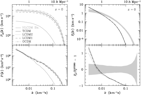
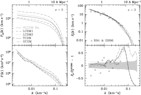
Figures 14 and 15 compare mass PSs and flux PSs for five simulations: HLCDM, LCDM1, high normalization LCDM (LCDM2), tilted LCDM (TCDM), and open CDM (OCDM). Table 1 lists the parameters for all these models. The $N$-body simulations all have the same box size of $22.222$ $h^{-1}$Mpc on each side and evolve $128^{3}$ CDM particles from $z=49$ to 0 using gadget (Springel, Yoshida & White, 2001). The initial conditions of these simulations have the same Fourier phases. Note that the TCDM model has an opposite tilt than HLCDM. Not all the simulations are consistent with most recent observations and they are provided only for testing the cosmological dependence of the flux PS.

Pseudo-hydro techniques have already been proven inaccurate at low redshift by several tests above. We include the results at $z=0$ here only to show that all the flux PSs based on the method DM-EOS are nearly indistinguishable from each other except the high normalization model LCDM2.

At $z=3$, the flux PS of the OCDM model departs from others at $k\ga 3$ $h$ Mpc^-1. However, this difference is not much more pronounced than those between the flux PSs obtained from the same simulation (HLCDM) but using different methods (see Figure 4). Moreover, if the flux PS is simply a linearized one-dimensional mass PS, one may expect that the order of the mass PS amplitudes should be preserved in the flux PS, but this is not observed in Figure 15. For example, the initial mass PS of LCDM2 (dotted lines) has the same shape as that of LCDM1 (dashed lines) but with a 56% higher normalization. This relative amplitude is preserved in the nonlinear three-dimensional PS and one-dimensional PS. However, as seen in the lower right panel, the flux PS of LCDM2 declines from 20% higher to 10% lower than that of LCDM1 from $k=0.002$ to $0.04$ km^-1s. This result is roughly consistent with that reported by McDonald et al. (2004b), who see a decline from 6% to -1% in the flux PS over the same range if the initial mass PS is boosted by 10%.

Without the detailed knowledge of the state of the IGM, one may confuse the differences between cosmological models (Figure 15) with the systematic errors of the pseudo-hydro methods (Figure 4). Therefore, to do precision cosmology with the Ly$\alpha$ forest without overly relying on hydrodynamical simulations, one should, at least, have precise calibrations of pseudo-hydro techniques.

5 Conclusions

Using hydrodynamical simulations and $N$-body simulations we find that pseudo-hydro techniques are able to reproduce the flux and flux PS at $k$ greater than a few $h$ Mpc^-1 that are obtained using the full-hydro method at $z=3$. There is also a good match between observed and simulated flux statistics such as the flux PS and its covariance at $z=3$. Since the performance of pseudo-hydro techniques improves toward higher redshift, we expect them to work even better at $z>3$.

For pseudo-hydro techniques, the mean-density temperature of the IGM does not affect the mean flux of the Ly$\alpha$ forest but it does alter the flux PS on small scales ($k\ga$ several $h$ Mpc^-1) through thermal broadening. The EOS of the IGM modifies both the amplitude and shape of the flux PS. We also observe a significant evolution in the shape of the flux PS from $z=0$ to 3 (e.g. Fig. 7).

The accuracy of pseudo-hydro techniques does not seem to be high enough for determining the Ly$\alpha$ flux PS at a few percent level. One needs to precisely calibrate pseudo-hydro techniques with hydrodynamical simulations. Moreover, it is better to constrain cosmology using the flux PS on scales above a few $h^{-1}$Mpc to reduce the uncertainties caused by the incomplete knowledge of the IGM.

To infer the one-dimensional linear mass PS one often divides the observed flux PS by the ratio between the simulated three-dimensional flux PS and the theoretical linear mass PS. This procedure is widely tested (e.g. Gnedin & Hamilton, 2002). In this way the sample variance error in the mass PS of the underly density field is avoided.

The transform from density to flux quenches fluctuations by orders of magnitude and leads to near-Gaussian Ly$\alpha$ fluxes. Hence, the variance of the flux PS is much less than that of the one-dimensional mass PS. In other words, one can measure the flux PS to a high precision with a relatively small number of LOSs but the underlying mass PS cannot be determined as precisely as the flux PS. Therefore, a large number of LOSs are needed to reduce the sample variance error in the one-dimensional mass PS, e.g. without binning the modes the standard deviation of the mean mass PS of 1024 LOSs is roughly 17% in a simulated cosmic density field at $z=3$ (Zhan & Eisenstein, 2005). Since the sample variance error in the one-dimensional mass PS is approximately inversely proportional to the number of LOSs, attempts to recover the three-dimensional mass PS accurate to 5% may require more than 10,000 LOSs. Such a large number of LOSs is very demanding, but is still within the reach of the Sloan Digital Sky Survey (SDSS). For instance, McDonald et al. (2004b) have used more than 3000 $z>2.3$ quasar spectra from the SDSS (over roughly a quarter of the targeted sky coverage) to estimate the linear mass PS. Thus, it is reasonable to project that there will be more than 10000 quasar spectra available when the SDSS finishes. Conversely, one can also trade resolution with precision by binning the modes and mitigate the demand for LOSs, even though binning highly correlated Fourier modes in the density field is not as efficient in reducing the sample variance error as binning independent ones.

The growing nonlinearity and non-Gaussianity at lower redshift drives up the cosmic variance of the mass PS and the correlation between different modes in the density field. This means that even more LOSs are needed to extend the Ly$\alpha$ flux PS analysis to low redshift. Fortunately, there are far more low-redshift quasar spectra available than high-redshift ones, although there will be many other astrophysical and observational challenges to be addressed. One such challenge is the inadequacy of the pseudo-hydro techniques at low redshift (Figure 3), when the shock-heated WHIM greatly alters the temperature–density relation of the IGM. A recent comparison between the HPM and full hydro methods confirms that it is the hot-phase gas that causes the differences between full and pseudo hydro results (Viel, Haehnelt & Springel, 2005). Thus it seems inevitable that time-consuming hydrodynamical simulations are needed to accurately model the low-redshift Ly$\alpha$ forest and to provide the means for inferring the mass PS and cosmological parameters.

References

- Bechtold (1994) Bechtold J., 1994, ApJS, 91, 1
- Bi & Davidsen (1997) Bi H. G., Davidsen A. F., 1997, ApJ, 479, 523
- Cen et al. (1994) Cen R., Miralda-Escudé J., Ostriker J. P., Rauch M., 1994, ApJ, 437, L9
- Croft et al. (1997) Croft R. A. C., Weinberg D. H., Katz N., Hernquist L., 1997, ApJ, 488, 532
- Croft et al. (1998) Croft R. A. C., Weinberg D. H., Katz N., Hernquist L., 1998, ApJ, 495, 44
- Croft et al. (1999) Croft R. A. C., Weinberg D. H., Pettini M., Hernquist L., Katz N., 1999, ApJ, 520, 1
- Croft et al. (2002) Croft R. A. C., Weinberg D. H., Bolte M., Burles S., Hernquist L., Katz N., Kirkman D., Tytler D., 2002, ApJ, 581, 20
- Davé & Tripp (2001) Davé R., Tripp T. M., 2001, ApJ, 553, 528
- Davé, Dubinski & Hernquist (1997) Davé R., Dubinski J., Hernquist L., 1997, New Astro., 2, 277
- Davé et al. (1997) Davé R., Hernquist L., Weinberg D. H., Katz N., 1997, ApJ, 477, 21
- Davé et al. (1999) Davé R., Hernquist L., Katz N., Weinberg D. H., 1999, ApJ, 511, 521
- Davé et al. (2001) Davé R., Cen R., Ostriker, J. P., Bryan G. L., Hernquist L., Katz N., Weinberg D. H., Norman M. L., O’Shea B., 2001, ApJ, 552, 473
- Dobrzycki & Bechtold (1996) Dobrzycki A., Bechtold J., 1996, ApJ, 457, 102
- Gnedin & Hamilton (2002) Gnedin N. Y., Hamilton A. J. S., 2002, MNRAS, 334, 107
- Gnedin & Hui (1998) Gnedin N. Y., Hui L., 1998, MNRAS, 296, 44
- Haardt & Madau (1996) Haardt F., Madau P., 1996, ApJ, 461, 20
- Hernquist et al. (1996) Hernquist L., Katz N., Weinberg D. H., Miralda-Escudé J., 1996, ApJ, 457, L51
- Hui (1999) Hui L., 1999, ApJ, 516, 519
- Hui & Gnedin (1997) Hui L., Gnedin N. Y., 1997, MNRAS, 292, 27
- Hui et al. (2001) Hui L., Burles S., Seljak U., Rutledge R. E., Magnier E., Tytler D., 2001, ApJ, 552, 15
- Katz, Weinberg & Hernquist (1996) Katz N., Weinberg D. H., Hernquist L., 1996, ApJS, 105, 19
- Kim et al. (2002) Kim T.-S., Carswell R. F., Cristiani S., D’Odorico S., Giallongo E., 2002, MNRAS, 335, 555
- Kim et al. (2004) Kim T.-S., Viel M., Haehnelt M. G., Carswell R. F., Cristiani S., 2004, MNRAS, 347, 355
- Lidz et al. (2005) Lidz A., Heitmann K., Hui L., Habib S., Rauch M., Sargent W. L. W., 2005, astro-ph/0505138
- Feng & Fang (2000) Feng L.-L., Fang L.-Z., 2000, ApJ, 535, 519
- Feng, Pando & Fang (2001) Feng L.-L., Pando J., Fang L.-Z., 2001, ApJ, 555, 74
- Lu et al. (1996) Lu L., Sargent W. L. W., Womble D. S., Takada-Hidai M., 1996, ApJ, 472, 509
- Mandelbaum et al. (2003) Mandelbaum R., McDonald P., Seljak U., Cen R., 2003, MNRAS, 344, 776
- McDonald (2003) McDonald P., 2003, ApJ, 585, 34
- McDonald & Miralda-Escudé (1999) McDonald P., Miralda-Escudé J., 1999, ApJ, 518, 24
- McDonald et al. (2000) McDonald P., Miralda-Escudé J., Rauch M., Sargent W. L. W., Barlow T. A., Cen R., Ostriker J. P., 2000, ApJ, 543, 1
- McDonald et al. (2004a) McDonald P., Seljak U., Cen R., Bode P., Ostriker J. P., 2004, submitted to MNRAS (astro-ph/0407378)
- McDonald et al. (2004b) McDonald P. et al., 2004, submitted to ApJ (astro-ph/0407377)
- Meiksin & White (2004) Meiksin A., White M., 2004, MNRAS, 350, 1107
- Monaghan & Lattanzio (1985) Monaghan J. J., Lattanzio J. C., 1985, A&A, 149, 135
- Nusser & Haehnelt (1999) Nusser A., Haehnelt M., 1999, MNRAS, 303, 179
- Penton, Stocke and Shull (2004) Penton S. V., Stocke J. T., Shull J. M., 2004, ApJS, 152, 29
- Petitjean, Mücket & Kates (1995) Petitjean P., Mücket J. P., Kates R. E., 1995, A&A, 295, L9
- Pichon et al. (2001) Pichon C., Vergely J. L., Rollinde E., Colombi S., Petitjean P., 2001, MNRAS, 326, 597
- Rauch et al. (1997) Rauch M. et al., 1997, ApJ, 489, 7
- Riediger, Petitjean & Mücket (1998) Riediger R., Petitjean P., Mücket J. P., 1998, A&A, 329, 30
- Seljak, McDonald & Makarov (2003) Seljak U., McDonald P., Makarov A., 2003, MNRAS, 342, L79
- Seljak et al. (2004) Seljak U. et al., 2004, submitted to Phys Rev D (astro-ph/0407372)
- Spergel et al. (2003) Spergel D. N. et al., 2003, ApJS, 148, 175
- Springel, Yoshida & White (2001) Springel V., Yoshida N., White S. D. M., 2001, New Astro., 6, 79
- Viel, Haehnelt & Springel (2005) Viel M., Haehnelt M. G., Springel V., 2005, submitted to MNRAS (astro-ph/0504641)
- Viel, Weller & Haehnelt (2004) Viel M., Weller J., Haehnelt M. G., 2004, MNRAS, 355, L23
- Viel et al. (2003) Viel M., Matarrese S., Theuns T., Munshi D., Wang Y., 2003, MNRAS, 340, L47
- Viel et al. (2004) Viel M., Matarrese S., Heavens A., Haehnelt M. G., Kim T.-S., Springel V., Hernquist L., 2004, MNRAS, 347, L26
- Viel et al. (2004) Viel M., Haehnelt M. G., Carswel R. F., Kim T.-S., 2004, MNRAS, 349, L33
- Zaldarriaga, Hui & Tegmark (2001) Zaldarriaga M., Hui L., Tegmark M., 2001, ApJ, 557, 519
- Zaldarriaga, Scoccimarro & Hui (2003) Zaldarriaga M., Scoccimarro R., Hui L., 2003, ApJ, 590, 1
- Zhan (2003) Zhan H., 2003, MNRAS, 344, 935
- Zhan & Eisenstein (2005) Zhan H., Eisenstein D., 2005, MNRAS, 357, 1387
- Zhan & Fang (2002) Zhan H., Fang L.-Z., 2002, ApJ, 566, 9
- Zhan, Jamkhedkar & Fang (2001) Zhan H., Jamkhedkar P., Fang L.-Z., 2001, ApJ, 555, 58
- Zhang, Anninos & Norman (1995) Zhang Y., Anninos P., Norman M. L., 1995, ApJ, 453, L57