[astro-ph/0503126] RECONSTRUCTION OF OBJECTS BY DIRECT DEMODULATION

1. Introduction

An observation to an object in space $x$ with an intensity distribution $f(\mbox{\boldmath$x$})$ can be seen as a modulation process of signal from object by observation instrument, the observed data $d(\mbox{\boldmath$\omega$})$ is an output after the modulation, where $\omega$ denotes the parameters determining the state of observation. The modulation equation relating the data to object can be written as

\int p(\mbox{\boldmath$\omega,x$})f(\mbox{\boldmath$x$})d\mbox{\boldmath$x$}=d(\mbox{\boldmath$\omega$})~{},

(1)

where a value $p(\mbox{\boldmath$\omega,x$})$ of the integral kernel (modulation function) is the modulation coefficient or response coefficient of the instrument to a point $x$ of the object space during an observation $\omega$ .

Generally, the data space $\omega$ is not the same kind of the object space $x$ . For an imaging formation system consisting of position-sensitive detectors, the data space $\omega=x^{\prime}$ is a two-dimensional space correspondent to the object space $x$ and the observed data $d(\mbox{\boldmath$x^{\prime}$})$ is an image of the object $f(\mbox{\boldmath$x$})$ , if the modulation function (point-spread function) is space-invariant, $p(\mbox{\boldmath$x^{\prime},x$})=p(\mbox{\boldmath$x^{\prime}-x$})$ , then the modulation equation (image formation equation) can be written as the following convolution formula

\int p(\mbox{\boldmath$x^{\prime}-x$})f(\mbox{\boldmath$x$})d\mbox{\boldmath$x$}\equiv p*f=d(\mbox{\boldmath$x^{\prime}$})~{}.

(2)

The image formation Equation (2) is a particular case of the general modulation Equation (1), and the image restoration (restoring the object $f(\mbox{\boldmath$x$})$ from the observed image $d(\mbox{\boldmath$x^{\prime}$})$ ), then, is a particular case of object reconstruction.

Dividing object space into $N$ bins, for $M$ observed values $d(k)$ , $k=1,...,M$ , the modulation Equation (1) or image formation Equation (2) in discretization form constitute an algebraic equation system

\sum_{i=1}^{N}p(k,i)f(i)=d(k)\hskip 14.22636pt(k=1,...,M).

(3)

In this paper we introduce the direct demodulation method of reconstructing object $f$ from observed data $d$ . This method can be applied to any kind of observation described by Equation (3). For a start we will give a brief summation of various reconstruction methods in classification.

2. Methods of Reconstruction

2.1. Linear Transformation

For observations by an image formation system, taking Fourier transforms of both sides of the image formation Equations (2) and taking advantages of the convolution theory of the Fourier transform, we have ${\cal F}p\cdot{\cal F}f={\cal F}d$ , then with the inverse transform the object can be derived as $f={\cal F}^{-1}({\cal F}d/{\cal F}p)$ .

In the case of observed values $d$ being projections, i.e. line integrals of object $f(\mbox{\boldmath$x$})$ along lines $L:a=\mbox{\boldmath$\xi$}\cdot\mbox{\boldmath$x$}$ (see Figure 1)

\int_{L_{a,\phi}}f(\mbox{\boldmath$x$})d\mbox{\boldmath$x$}=\int_{L_{a,\phi}}f(\mbox{\boldmath$x$})\delta(a-\mbox{\boldmath$\xi$}\cdot\mbox{\boldmath$x$})d\mbox{\boldmath$x$}=d(a,\phi)

then $d$ is a sample of the Radon transform (Radon 1917), $d={\cal R}f$ , with the inverse transform we can reconstruct the object from projections, $f={\cal R}^{-1}d$ . The Radon transform is the mathematical basis of the computerized tomography (CT) technique.

Refer to caption — Figure 1.: Projection along line $L$ in two-dimensional Radon transform.

The cross-correlation function

c(\mbox{\boldmath$x$})=\int p(\mbox{\boldmath$\omega,x$})d(\mbox{\boldmath$\omega$})d\mbox{\boldmath$\omega$}

(4)

is a distribution in the object space. In general case we can use the correlation calculation to perform transformation from data space to object space. Correspondent to the modulation Equation (3), the discrete correlation transform is

c(i)=\sum_{k}p(k,i)d(k)~{}.

(5)

There exists another form of correlation transform defined as

	$\displaystyle c^{*}(i)$	$\displaystyle=$	$\displaystyle\frac{A}{M}\sum_{k=1}^{M}(p(k,i)-\bar{p})(d(k)-\bar{d})$		(6)
		$\displaystyle=$	$\displaystyle A^{\prime}[M\sum_{k}p(k,i)d(k)-\sum_{k}p(k,i)\sum_{k}d(k)]~{}.$		(6)

If the object is an isolated point source with intensity $f_{s}$ at point $i_{s}$ , then the correlation function $c^{*}(i)=f_{s}\cdot c_{s}(i;i_{s})$ , where $c_{s}(i;i_{s})$ is the resolution function for point $i_{s}$

c_{s}(i;i_{s})=A^{\prime}[M\sum_{k}p(k,i)p(k,i_{s})-\sum_{k}p(k,i)\sum_{k}p(k,i_{s})]~{}.

(7)

The distribution of $c^{*}(i)$ will appear a bulge around the bin $i_{s}$ , provided that the observations get necessary information of object (the observations are properly arranged and the number $M$ of observations is large enough). The normalization constant can be chosen as $A^{\prime}=1/[M\sum_{k}(p(k,i))^{2}-(\sum_{k}p(k,i))^{2}]$ , then the maximum value of the correlation function, $c^{*}(i_{s})$ , equals the source strength, $f_{s}$ . The width of the resolution function $c_{s}(i)$ represents the resolution ability of the observations, which can be defined as the intrinsic resolution of the observations.

2.2. Statistical Reconstruction

Another important category of reconstruction methods is to use a certain statistic (e.g. the maximum likelihood ratio (Pollock et al. 1981)) instead of the object itself to represent main characters of object by some degree or to use values of a statistic (e.g. the $\chi^{2}$ quantity) instead of the observation modulation equations in selecting possible object distributions. If the object distribution can be described by a theoretical or empirical expression $f(i)=g(i;\mbox{\boldmath$a$})$ , where $\mbox{\boldmath$a$}=(a_{1},...,a_{l})$ are $l$ undetermined parameters, the least-squares reconstruction $g(i;\mbox{\boldmath$a$})$ $(i=1,...,N)$ satisfies the condition

\chi^{2}(\mbox{\boldmath$a$})=\sum_{k}\{[d(k)-\sum_{i}p(k,i)g(i;\mbox{\boldmath$a$})]/\sigma_{k}\}^{2}=\min

with $\sigma_{k}$ being the statistical error of $d(k)$ . The maximum-entropy method (for example, see Gull & Daniell 1978) is to choose a solution $f(i)~{}(i=1,...,N)$ from all satisfying the statistical criterion

\chi^{2}(\mbox{\boldmath$f$})=\sum_{k=1}^{M}\{[\sum_{i}p(k,i)f(i)-d(k)]/\sigma_{k}\}^{2}=M

by the condition that the information entropy

S(\mbox{\boldmath$f$})=-\sum_{i}f_{i}\log f_{i}=\max.

2.3. Direct Demodulation

The most straightforward way to evaluate an object $f$ from observed data $d$ should be directly solving the modulation equation connecting $d$ with $f$ , i.e. direct demodulation, which we will discuss in this paper.

Using a statistic instead of original modulation equations to make reconstruction will cause loss of information containing in the equations about object and observations, then that of sensitivity and resolution ability of reconstruction. The least-squares method is model dependent, not applicable in general case. Reconstruction by Fourier or Radon transform is mathematically based on modulation equation, but only can work on a special kind of observation, i.e. image formation or projection. In application of Fourier or Radon transform to incomplete and noisy data in practice, in particular to that with poor statistics and low ratio of signal to noise, in order to derive a reasonable reconstruction a certain treatment (e.g. frequency space filtering) should be applied, causing loss of information. Correlation calculation can perform transformation from data space to object space in general case, thus being a useful tool in dealing with reconstruction problems; but the correlation function $c(i)$ or $c^{*}(i)$ is not a good representation of an object, there may exist regions with negative $c^{*}(i)$ even if the object is defined only in a positive space.

Before introducing the direct method of reconstruction, we will firstly compare various methods of solving a linear equation system.

3. Solutions of Linear Algebraic Equations

The modulation equation system (3) can be rewritten in matrix form as

\mbox{\boldmath$Pf=d$}~{},

(8)

where modulation matrix $\mbox{\boldmath$P$}=\{{p(k,i)}\}$ , object vector $\mbox{\boldmath$f$}=\{f(i)\}$ , data vector $\mbox{\boldmath$d$}=\{d(k)\},i=1,...,N,k=1,...,M.$

3.1. Mathematical Solution

If the modulation matrix $P$ is non-singular and $M=N$ , the exact solution of Eq.(8), $\mbox{\boldmath$f=P$}^{-1}\mbox{\boldmath$d$}$ , can be found by Gaussian elimination or triangular resolution. Iterative method can also be used to solve Eq.(8). An iteration algorithm in common use is the Gauss-Seidel method with successive relaxation. The approximate solution for $l$ -th iteration can be calculated by one of the following two formulas

	$\displaystyle f_{i}^{(l)}$	$\displaystyle=$	$\displaystyle\alpha(d_{i}-\sum_{j=1}^{i-1}p_{ij}f_{j}^{(l)}-\sum_{j=i+1}^{N}p_{ij}f_{j}^{(l-1)}+(1-p_{ii})f_{i}^{(l-1)})+(1-\alpha)f_{i}^{(l-1)}$		(9)
	$\displaystyle f_{i}^{(l)}$	$\displaystyle=$	$\displaystyle\frac{\alpha}{p_{ii}}(d_{i}-\sum_{j=1}^{i-1}p_{ij}f_{j}^{(l)}-\sum_{j=i+1}^{N}p_{ij}f_{j}^{(l-1)})+(1-\alpha)f_{i}^{(l-1)}$		(10)

where the relaxation factor $0<\alpha\leq 1$ . It can be proved that the Gauss-Seidel iteration converges to the exact solution if the matrix $P$ is symmetry and positive definite.

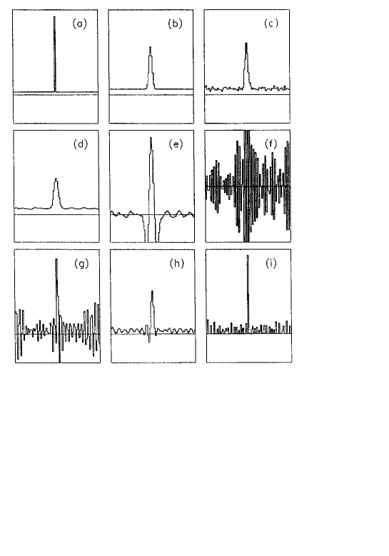
The mathematical solution of a modulation equation system satisfy the equations accurately. But there always exist errors in modulation equations (measurement errors, statistical fluctuation and noises in data and errors in determining modulation coefficients). A modulation equation system in a practical problem is usually a large set of linear equations, its mathematical solutions will seriously deviate from the true object distribution due to errors in the equations. A one-dimensional example is displayed in Figure 2: (a) is an object distribution $f$ , a line at $i_{0}$ on a uniform background; (b) the ideal data $d_{0}(k)=\sum_{i}p(k,i)f(i)$ , where the triangular distribution presents the shape of the modulation function $p(k,i_{0})$ ; (c) the simulated observed data $d$ , a Monte Carlo sample from (b); (d) and (e) are the correlation distribution $c(i)$ and $c^{*}(i)$ respectively; (f) presents the mathematical solution of the modulation equations $Pf=d$ by Gauss-Seidel iterations. From Figure 2f we can see that the mathematical solution of the modulation equations with statistical errors is in an ill-conditioning feature with violent oscillation, including a lot of nonphysical values of $f<0$ .

3.2. Statistical Solution

If the number of observed values is greater than that of the undetermined parameters, $M>N$ , the system (3) is overdetermined, we can use the least-squares criterion $\sum_{k}[\sum_{i}p(k,i)f(i)-d(k)]^{2}=$ min to derive the normal equations as

\sum_{i=1}^{N}p_{1}(i^{\prime},i)f(i)=c_{1}(i^{\prime})\hskip 14.22636pt(i^{\prime}=1,...,N),

(11)

where $p_{1}(i^{\prime},i)=\sum_{k}p(k,i^{\prime})p(k,i)$ , the right side of the normal equation is the correlation function $c_{1}(i^{\prime})\equiv c(i^{\prime})=\sum_{k}p(k,i^{\prime})d(k)$ . The mathematical solution of the normal Equations (11), i.e. the least-squares solution of the modulation Equations (3), can be taken as an estimation of object in a sense of least-squares (in a statistical sense).

The normal equations are just the correlation transform of the original modulation Equations (3), we can call them correlated modulation equations. For the case of $M\leq N$ we can also derive equations of the same form by means of correlation transformation. The correlation transformation can be repeatedly performed (Li & Wu 1992, 1993). Starting from the original modulation eqs. (3), after $L$ -fold correlation transforms we can obtain the $L$ -order correlated modulation equations as

\sum_{i=1}^{N}p_{L}(i^{\prime},i)f(i)=c_{L}(i^{\prime})\hskip 14.22636pt(i^{\prime}=1,...,N),

(12)

where $p_{L}(i^{\prime},i)=\sum_{j}p_{L-1}(j,i^{\prime})p_{L-1}(j,i),c_{L}(i^{\prime})=\sum_{j}p_{L-1}(j,i^{\prime})c_{L-1}(j)$ .

Figure 2g and 2h show the solutions of correlated modulation equations of $L=1$ and $L=2$ , respectively (statistical solutions of modulation equations).

3.3. Physical Solution (Constrained Iterative Solution)

Setting reasonable physical constraints in the iterative process of solving a modulation equation system (3) or correlated modulation equation system (12) will help us obtain an estimation of the object distribution satisfying some necessary physical conditions (Li & Wu 1992,1993). Corresponding to a certain object, we can set up a lower bounds $b$ and upper bounds $u$ , for any approximate solution $f^{(l)}(i)$ ,

	$\displaystyle if\hskip 5.69054ptf^{(l)}(i)$	$\displaystyle<$	$\displaystyle b(i),\hskip 8.53581ptlet\hskip 5.69054ptf^{(l)}(i)=b(i),$
	$\displaystyle if\hskip 5.69054ptf^{(l)}(i)$	$\displaystyle>$	$\displaystyle u(i),\hskip 8.53581ptlet\hskip 5.69054ptf^{(l)}(i)=u(i).$		(13)

The final solution should be normalized by the condition $\sum_{k}\sum_{i}p(k,i)f(i)=\sum_{k}d(k)$ . For many objects, nonnegativity is a necessary constraint, i.e. $b(i)=0,(i=1,...,N)$ . Figure 2i is a constrained iterative solution for data (c) under the nonnegative condition after $10^{2}$ iterates. The constrained iteration process has a good property of convergence and is not sensitive to small errors in the modulation function. We found the approximate solution after $10^{4}$ or more iterates or that starting from completely different initial values had not any recognized difference with Figure 2i. When the modulation function used in iteration being widened in a direction and narrowed in the other direction by $20\%$ separately, no obvious change was found in the constrained iterative solution, and when the whole modulation function being widened by $20\%$ also almost the same figure of solution was obtained but just the peak height increased a little.

Exerting the constraints of lower and upper bounds is a kind of nonlinear control in the iterative precess, proper nonlinear control can depress the influence of noise, fluctuation and other errors in data effectively and strengthen convergence of the iterative process, helping to derive a satisfactory reconstruction in a physical sense. There exist various iterative algorithms applicable to seeking physical solutions. The modulation matrix $p_{L}$ of the correlated modulation Equations (12) is symmetry and positive definite, satisfying convergence condition of the successive relaxation Gauss-Seidel iteration. Another useful algorithm is the Richardson-Lucy iteration (Richardson 1972; Lucy 1974) based on the Bayes theory

f^{(l)}(i)=f^{(l-1)}(i)\sum_{k}\frac{p(k,i)d(k)}{\sum_{i^{\prime}}p(k,i^{\prime})f^{(l-1)}(i^{\prime})}/\sum_{k}p(k,i)~{}.

(14)

Solutions from probability iterations satisfy the nonnegative condition and normalization condition of total flux automatically. However, only nonnegative constraint is not enough to control the iterative process to produce a satisfactory reconstruction from many observations, in particular from that of poor statistics and low ratio of signal to noise for complicated objects. In the case of object space including negative area, the simple nonnegative constraint can not be used at all.

Relaxation functions to modify the correction term gradually as iteration proceeds were suggested for spectral deconvolution (for example, see Jansson 1984). In oder to fulfil a need for setting various kind of physical constraints necessary in practice we proposed to set boundary constraints directly on each approximate solution as shown by expression (13) and found that a direct demodulation method in the general case can be constituted by this technique, which we will introduce in the following section.

4. Direct Demodulation Method

It is obvious that in solving modulation Equations (3) or correlated modulation Equations (12) taking the intensities $\mbox{\boldmath$f$}_{b}$ of the diffuse background in the object space as lower bounds, i.e.

b=f_{b}

(15)

can make more precise control than using simple nonnegative constraint, giving a better estimation of the object.

In the case of no priori knowledge of the diffuse background, it is needed to estimate it from observed data. First we use a successive procedure similar to CLEAN (Högbom 1974) to subtract all contribution of apparent discrete sources with intensities greater than $f_{m}$ from the observed data $d$ and derive background data $d_{b}$ , where $f_{m}$ can be taken as the minimum intensity of discrete sources to be reconstructed. Solving the modulation equations for $d_{b}$ , $Pf_{b}=d_{b}$ , by an iterative method we finally get $f_{b}$ . In iterations we can simply smooth each approximate solution $f_{b}^{(l)}$ or use some kind of continual condition like

u(i)=f_{b}^{(l)}(i-1)+\delta,\hskip 8.53581ptb(i)=f_{b}^{(l)}(i-1)-\delta

(16)

to depress sudden change of intensity at any point $i$ from its close neighbour one $i-1$ in the object space, where $\delta=f_{m}/n_{b}$ with $n_{b}$ being the linear size of minimum diffuse structure reconstructed by number of bins.

Subtracting contribution of apparent discrete sources from data can be performed with the aid of cross-correlation technique. Find out the maximum point $i_{s}$ of the correlation map $c^{*}(i)$ $(i=1,...,N)$ for data $d$ and the intensity excess $f_{s}$ above the background level at $i_{s}$ , remove the contribution of $f_{s}$ from the data by $d_{b}(k)=d(k)-p(k,i_{s})f_{s}$ , $(k=1,...,M)$ . The procedure is repeated for $d_{b}$ till $f_{s}<f_{m}$ . The excess $f_{s}$ can be determined by the condition $\sum_{i^{\prime}}(c_{b}(i^{\prime})-[c^{*}(i^{\prime})-f_{s}c_{s}(i^{\prime},i_{s})])^{2}=min$ , where the sum for $i^{\prime}$ is accumulated over a region around $i_{s}$ within the width of the resolution function, $c_{b}(i^{\prime})$ is the extrapolated value of correlated intensities $c^{*}(i)$ outside the region to the point $i^{\prime}$ .

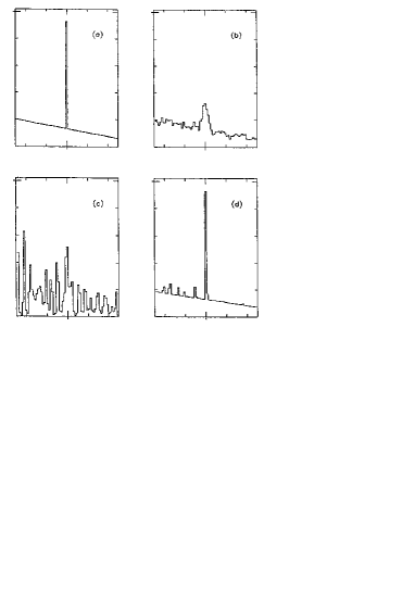
An example of restorations of a line source superimposed on an inclined background is shown in Figure 3: (a) is the object distribution, (b) the simulated data, (c) Richardson-Lusy iterative restoration (i.e. a constrained iterative solution of modulation equations with only the nonnegative condition), (d) restoration by the direct demodulation for correlated modulation equations of $L=1$ .

For many reconstruction problems in practice, performing iterations in two steps with the constraint condition (16) and (15) separately by the Gauss-Seidel formula with successive relaxation to the correlated modulation Equations (12) of $L=1$ , or by the Richardson-Lucy formula to the original modulation Equations (3), one can get satisfactory reconstructions. In the case of data having good statistics, solving the original modulation Equations (3) by constrained Gauss-Seidel iterations will give high resolution reconstruction; but in the other hand, for observations with severe noise and fluctuation and bad intrinsic resolution, higher order correlated modulation Equations (12) can serve to get better reconstruction. In iterations for reconstructing diffuse background correlated modulation equations of higher order are also recommended.

5. Modulation Imaging

The direct demodulation method can be applied to dealing with various kind of reconstruction problems, i.e. to solving the inverse problems of the general modulation Equations (3), where the data space determined by apparatus and states of observation can be completely different with the observed object space $x$ , and the number of observations, $M$ , is not necessary to be equal to or greater than that of undetermined parameters, $N$ (Li et al. 1993). A general demodulation technique make it possible to design an experiment by simple instrument to realize the same objective as more complicated one does, for example, to obtain a two-dimensional image by a one-dimensional non-position-sensitive detector ( non-imaging system).

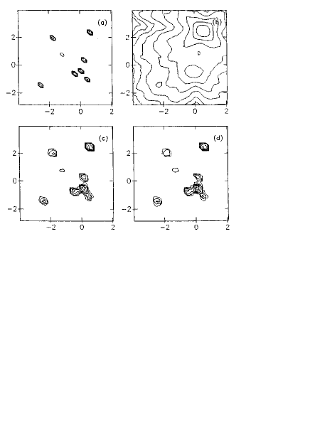
We made Monte Carlo simulations to study the imaging capability of a simple collimated hard X-ray telescope consisting of two 700 cm² non-position-sensitive scintillators, each in viewed by just a single photomultiplier tube (PMT) and modulated by a slat collimator of $5^{o}\times 0.5^{o}$ and $0.5^{o}\times 5^{o}$ (FWHM) aperture separately (sketched in Figure 4). The object scene (Figure 5a) in our simulations is the galactic center region containing eight point sources which was observed by a coded mask telescope flown on the Spacelab 2 mission (Skinner et al. 1987). The strongest source intensity was $7.05\times 10^{-2}$ cm^-2 s^-1, the ratio of the strongest source intensity to the weakest was 100:1, the background was taken as 0.089 counts cm^-2 s^-1 as estimated from the observation. A 24 hours survey by the collimated telescope was simulated: pointing to various sky points over a $6^{o}\times 6^{o}$ region around the Galactic Center separated by $1^{o}$ along the galactic longitude $l$ or latitude $b$ between two successive ones, during each pointing producing the output counts of each detector for eight different places of the telescope $xy$ plane rotated around the $z$ axis by Monte Carlo simulation. Figure 5b is the cross-correlation map from the simulated data. A reconstruction by the direct demodulation technique is shown in Figure 5c, which seems even better than the simulated image of the same object scene by a 1473 cm² coded mask telescope with $93\times 99$ detector pixels for 24 hours observation (Lei et al. 1991).

For studying the effect of background variation on modulation imaging, we doubled the background intensity when the telescope pointing to $(l,b)=(1.0^{o},-1.0^{o})$ but no recognizable change was produced in the resultant image. In addition we assumed that starting from the pointing $(l,b)=(1.0^{o},-1.0^{o})$ the background intensity was linearly increasing with the passage of time up to three times and then gradually decreasing back to the initial level, the whole variation lasted one hour, the corresponding direct reconstruction is shown in Figure 5d.

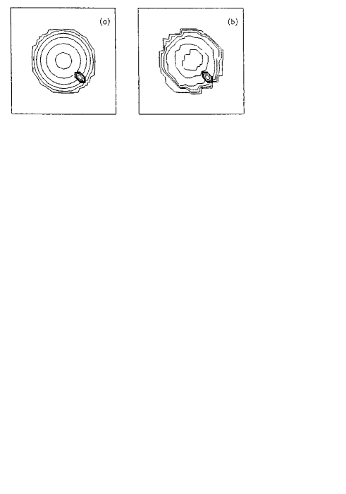
The modulation imaging has a capability to simultaneously reconstruct both extended and discrete features in object. We simulated scan observations of the object scene of $10^{o}\times 10^{o}$ shown in Figure 6a by the collimated telescope (Figure 4) with step of $1^{o}$ , Figure 6b is the direct demodulation image from the simulated data.

6. Discussion

The direct demodulation, directly solving modulation equations and directly controlling each iterative output by physical conditions, is a flexible technique: in accordance with different characters of object, instrument and state of observation and different requirement for reconstruction corresponding algorithms can be designed, and various kind of priori knowledges can be easily included in modulation equations or constraint conditions as well.

The modulation Equation (1), observed data $d(\mbox{\boldmath$\omega$})$ being an weighted sum (integral) of an object $f(\mbox{\boldmath$x$})$ over any region with a weight function (integral kernel) $p(\mbox{\boldmath$\omega,x$})$ of any form, can represent a measurement process in very general case, thus the direct demodulation method can be applied to general reconstruction problems. The CT imaging is only a special case of general modulation imaging: the observed data are projections of object; in other words, the CT technique can be used only to a special case of the modulation Equation (1) where the integral kernel (modulation function) is a kind of $\delta$ function.

Each iterative calculation in direct demodulation is directly based on the modulation equation. Obviously the direct approach can use the information containing in the modulation equations more sufficiently than any indirect one through a statistical criterion or cross-correlation transformation, that is the main reason of the resolution of a direct reconstruction being able to be much better than the intrinsic resolution (compare Figure 2i with 2e and Figure 5c with 5b). For ideal data without error and with necessary information of object, i.e. the modulation matrix $P$ being non-singular (observations properly arranged) and its rank $M\geq N$ (number of observations large enough), solving the modulation equations will precisely reconstruct the object, e.g. solving $\mbox{\boldmath$Pf=d$}_{0}$ can exactly restore Figure 2a from Figure 2b no mater how wide the resolution function $p(k,i_{0})$ is.

The main difficult of the direct method is the illness of solution causing by errors in data. Introducing physical constraints to make nonlinear control in the process of solving modulation equations and using correlation transformation properly can depress the effect of errors effectively and then make high resolution direct reconstruction realizable.

The physical solution resulted from solving a modulation equation system under physical constraints is neither a solution in a strictly mathematical sense nor the statistical solution in a least-squares sense. Neither the modulation equations nor the normal equations are satisfied by the physical solution. Studying the mathematical properties of physical solutions is a difficult problem of nonlinear mathematics. The quality of a direct reconstruction (sensitivity, resolution, uncertainty, etc.) depends on the quality and quantity of information about the object containing in the observed data as well as the ratio of signal to noise, and relates to the ability of the signal modulation pattern depressing noises. The generality of the direct demodulation technique implies that various kind of apparatus (detectors and modulators) constituted by different principles can be selected for observing the same object. Until now no general mathematical method can guide us to designing modulators and arranging observations, even not a clear standard to judge the quality of a reconstruction. How many observations are necessary for reconstruction depends on properties of observation system, arrangement of observations and characteristics of observed object (size of reconstructed space and complexity of object), and also relates to requirements for reconstruction. Just from resolution consideration we may arrange observations properly and take the number $M$ of observations sufficiently large to make the intrinsic resolution function (7) fine enough (comparing with the achievable limit of the instrument).

Designing detector and modulator and estimating statistical errors and other uncertainties in a reconstruction can be aided by simulation calculations. Statistical uncertainties can be evaluated by the bootstrap method (Efron 1979; Diaconis & Efron 1983), estimating other uncertainties and comparing different observation instruments and arrangements can be made by Monte Carlo simulations. In performing direct demodulation by a computer, the computation is quite fast as the algorithm is constituted by only simple arithmetic operations and conditional control statements, although a larger space of the main storage is often needed to store modulation coefficients and reconstruction results. It is feasible in many practical cases to study the direct demodulation through simulation calculations for Monte Carlo samples or bootstrap samples.

The authors thank Prof. Jun Nishimura for helpful discussion. This work was supported by the National Natural Science Foundation of China.

References

Diaconis P. & Efron B.: 1983, Scien. Am., Sept. p.96.

Efron B.: 1979, Ann. Statistics, 7, 1.

Gull S.F. & Daniell G.J.: 1978, Nature 272, 686.

Högbom J.A.: 1974, Astron. Astrophys. Suppl. 15, 417.

Jansson P.A.: 1984, Deconvolution with Application in Spectroscopy, Academic Press.

Lei F., Fraser-Mitchell J. & Learworth M.: 1991, Exper. Astron. 1, 285.

Li T.P. & Wu M.: 1992, in Astronomical Data Analysis Software & Systems I, ed. Worrall D.M., Biemesderter C. & Barnes J., 229.

Li T.P. & Wu M.: 1993, Astrophys. Space Sci. 206, 91.

Li T.P., Wu M., Lu Z.G., Wang J.Z. & Zhang C.S.: 1993, Astrophys. Space Sci. 205, 381.

Lucy L.B.: 1974, Astron. J., 79, 745.

Pollock A.M.T., Bignami G.F., Hermsen W., Kanbach G. & Lichti G.G.: 1981, Astron. Astrophys. 94, 116.

Radon J.: 1917, Berichte Sächsische Academie der Wissenschaften. Leipzig,

Math.-Phys. Kl. 69, 262.

Richardson B.M.: 1972, J. Opt. Soc. Am. 62, 55.

Skinner K.K. et al.: 1987, Nature 330, 544.

RECONSTRUCTION OF OBJECTS BY DIRECT DEMODULATION

Abstract