The interaction of a jet-like pulse with a wind from a stellar companion

Abstract

We present numerical simulations of the interaction between a collimated, bipolar “pulse” ejected from a star and a continuous wind ejected from a stellar companion. We explore the characteristics of the predicted H$\alpha$ intensity maps by varying selected input parameters. We find that the asymmetry (in size and strength) between the two lobes of the proto-planetary nebula OH 231.8+4.2 is reproduced in this scenario if the wind ejected by the companion star has a strong latitude dependence.

Presentamos simulaciones numéricas de la interacción entre un “pulso” bipolar colimado expulsado por una estrella y el viento continuo debido a una estrella compañera. Se muestra la variación de las propiedades de los mapas de intensidad en H$\alpha$ al variar los valores de algunos de los parámetros de entrada. Mostramos que la asimetría (en el tamaño y la intensidad) entre los dos lóbulos de la nebulosa proto-planetaria OH 231.8+4.2 se puede explicar en el escenario propuesto si el viento de la estrella compañera muestra una fuerte dependencia con la latitud.

ISM: kinematics and dynamics - PLANETARY NEBULA: individual (OH231.8+4.2) 0.9

0.1 Introduction

Most proto-planetary Nebulae (PPNe) show bipolar or mutipolar lobes, highly collimated outflows or jets and other complex structures. A particularly well studied PPN candidate is the nebula associated with the OH 231.8+4.2 source. This is a remarkable example of a bipolar PPNe with collimated outflows. In H$\alpha$ and forbidden emission line maps, this object presents a clear axial symmetry with the existence of shocked material in a wide, bipolar bubble with an obscuring ridge in between the two lobes (Bujarrabal et al. 2002). Long-slit spectra of this object show the presence of Herbig-Haro like knots at the end of the bipolar lobes, which probably trace the interaction between the fast, collimated molecular jet and the ambient material (Sánchez Contreras et al. 2000a). Contrary to what happens in most PPNe, the two optical lobes have different sizes; the Southern lobe is weaker but about two times more extended than the Northern lobe (Reipurth 1987; Sánchez Contreras et al. 2000a).

In the optical and NIR continuum, the nebula is narrow and elongated along its symmetry axis (Alcolea et al. 2001; Meakin et al. 2003). The same narrow component is observed in CO and other molecular emission lines (Alcolea et al. 2001; Sánchez Contreras, Bujarrabal & Alcolea 1997; Sánchez Contreras et al. 2000b). The kinematical properties of this molecular jet are remarkable; its velocity increases linearly with distance from the star following a Hubble-like velocity law, which is consistent with a sudden acceleration event (Alcolea et al. 2001; Alcolea 2004). The Southern molecular jet (as seen in CO emission) is clearly more extended than the Northern jet and shows the highest flow velocity. The deprojected velocities show values of up to 430 km s^-1 in the Southern jet, and up to 210 km s^-1 in the Northern jet (Alcolea et al. 2001). The length along the axis of the OH 231.8+4.2 nebula is $\sim$50^′′, which at a distance of 1.5 kpc (Kastner et al. 1992) implies a length $>10^{18}$ cm.

The central source of OH 231.8+4.2 is not detected at optical wavelengths because of the dusty envelope, but the reflected light has a M9 III spectral type, with a blue excess that suggests the presence of a warmer companion (or a peculiar photospheric structure and/or an accretion disk; Cohen 1981). This star is a typical Mira variable at the end of the Asymptotic Giant Branch (AGB) identified with QX Pup (Kastner et al. 1998). Recently, OH 231.8+4.2 has been mapped at high spatial resolution in SiO and H₂O maser emission (Sánchez Contreras et al. 2002; Gómez & Rodríguez 2001). The position of the SiO and H₂O masers (which are tracing the position of QX Pup), are clearly offset from the axis of the bipolar outflow (as first pointed out by Gómez & Rodríguez 2001).

The QX Pup star shows the variability and maser emission properties typical of a Mira star (or of an OH/IR star) at the AGB. The contradiction between the apparent evolutionary stage of the nebula (i.e., PPN) and that of the QX Pup (AGB) star has been discussed by many authors (see, e.g., Alcolea et al. 2001). Based on the large displacement ($>1000$ AU) between the position of the SiO maser and the bipolar axis of the nebula, Alcolea (2004) has proposed that QX Pup may not be directly related to the bipolar nebula. As first pointed out by Alcolea (2004), if the QX Pup star were located in the Northern lobe the observed differences between the two lobes possibly could be explained as a result of the interaction between the northern lobe and the wind from QX Pup.

In this paper, we present 3D numerical simulations of the interaction between a collimated, bipolar “pulse” ejected from a star and a continous wind ejected from a stellar companion. These simulations are a first attempt to reproduce the asymmetry between the two lobes of the bipolar PPN OH 238.1+4.2 in terms of a bipolar outflow/stellar wind interaction model. From the numerical simulations, we obtain predictions of H$\alpha$ maps that can be compared with the optical images of OH 238.1+4.2 (Sánchez Contreras et al. 2000a; Bujarrabal et al. 2002).

The paper is organized as follows. In § 2 we describe the parameters and the numerical method which have been used. In § 3 we present the results of the numerical simulations. In § 4 we compare our simulations with the observations of the PPN OH 231.8+4.2.

0.2 The numerical models

0.2.1 General considerations

We compute a series of five models of the interaction between a collimated, bipolar “pulse” ejected from a star and a continuous wind ejected from a stellar companion. The models are computed in a 3D cartesian coordinate system, with its origin centered in the middle of the computational domain. The domain has a physical extent of $1.5\times 10^{18}$ cm along the $z$-axis, and of $7.5\times 10^{17}$ cm along the $x$- and $y$-axes. Outflow conditions are applied in all of the domain boundaries.

The computations are carried out with the “yguazú-a” code, which integrates the gasdynamic equations in a binary, adaptive computational grid. This code is described in detail by Raga, Villagrán-Muniz & Navarro-González (2000). In the version of the code that we have employed, a single rate equation for neutral hydrogen is integrated (together with the 3D gasdynamic equations), and a simplified cooling function is calculated as a function of the density, ionization fraction and temperature (as described by Raga et al. 2000). This cooling function is then added as a sink term in the energy equation.

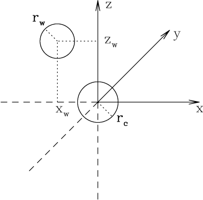
For our simulations, we have used a 5-level binary grid with a maximum resolution of $5.86\times 10^{15}$ cm along the three axes. The domain was initialized with a wind solution (§2.2) and a “bipolar pulse” (§2.3), and the simulations were carried out until the shell pushed out by the “pulse” reaches one of the boundaries of the computational domain. The initial flow configuration is shown in Figure 1.

Figure 1: Schematic diagram showing the configuration used for the numerical simulations (see the text). A collimated wind “pulse” is initialized within a sphere of radius $r_{c}$ (centered at the origin of the coordinate system) and the continuous wind from the stellar companion is imposed (at all times) within a sphere of radius $r_{w}$, which is centered at the point $(x_{w},0,z_{w})$. In the diagram, the projections of these two spheres on the $xz$-plane are shown. The axis of the “pulse” (as well as the axis of the wind in the simulations with a latitude-dependent wind) is parallel to the $z$-axis.

0.2.2 The wind

We have initialized the computational domain with a wind with a latitude-dependent density of the parametrized form :

$$\rho={{\dot{M}}_{w}\over 4\pi r^{2}}\,f(\theta)\,,$$ (1)

where $r$ is the spherical radius measured from the position of the wind source. The wind has an outward directed velocity (independent of $r$) given by :

$$v={v_{w}\over f(\theta)}\,,$$ (2)

with $v_{w}=40$ km s^-1 for all of the computed models, and with different values of ${\dot{M}}_{w}$ for the successive models (see Table 1). The anysotropy function $f(\theta)$ has the parametrized form :

$$f(\theta)=\xi-(\xi-1)\cos^{p}\theta\,,$$ (3)

where $\theta$ is the angle measured from the polar axis of the wind (which we take to be parallel to the $z$-axis of the computational domain), $\xi$ is a constant which is equal to the equator-to-pole density ratio, and $p$ is a constant which determines the degree of flattening towards the equator of the density stratification. As can be seen from Equation (3), a wind with $\xi=1$ is isotropic. The choices of $\xi$ and $p$ for the computed models are given in Table 1.

7 Model ${\dot{M}}_{w}$a $x_{w}$b $z_{w}$b $\xi$c $p$c $t_{f}$d [$10^{-6}$M_⊙yr^-1] [$10^{17}$cm] [yr] M1 01 $-1.0$ 1.5 01 — 1100 M2 05 $-1.0$ 1.5 01 — 1500 M3 03 $-1.0$ 1.5 20 0.5 1500 M4 10 $-3.0$ 1.5 20 0.5 2300 M5 10 $-3.0$ 1.5 50 0.5 2700 aMass loss of the wind from the stellar companion bPosition on the $xz$-plane of the stellar wind source cAsymmetry parameters of the wind dTime at which the expanding shell starts to leave the computational grid (the frames of figures 2-6 correspond to these times)

Table 1: Collimated pulse/wind interaction models

The source of the wind is located at a position $(x_{w},0,z_{w})$ away from the origin of the coordinate system (which is at the center of the computational domain, see Figure 1 and §2.1). The values of $x_{w}$ and $z_{w}$ chosen for the computed models are given in Table 1. The whole of the computational domain (with the exception of the region occupied by the “bipolar pulse”, see §2.3) is initialized with the wind solution, with the density and velocity given by Equations (1-3). Also, the wind solution is imposed at all times within a sphere of radius $r_{w}={2.5\times 10^{16}}$ cm, centered on the $(x_{w},0,z_{w})$ source position (see Figure 1).

We impose a uniform, $T_{w}=10^{3}$ K within the sphere of radius $r_{w}$, and a temperature

$$T=T_{w}\,\left({r_{w}\over r}\right)^{2(\gamma-1)}\,,$$ (4)

outside of this sphere, where $T_{w}$ and $r_{w}$ are constants defined above, $\gamma=5/3$ is the specific heat ratio and $r$ is the spherical radius measured from the position of the wind source. This temperature stratification (corresponding to a constant velocity, adiabatic wind) is of course only used in the $r>r_{w}$ region as an initial condition. Finally, the ejected wind is assumed to have fully neutral H, and to have a small, seed ionization fraction coming from singly ionized C.

0.2.3 The bipolar pulse

As an initial condition, we impose a “bipolar pulse” of material ejected from a source located at the origin $(x,y,z)=(0,0,0)$ of the coordinate system (see Figure 1). This bipolar “pulse” is imposed as an initial condition within a sphere of radius $r_{c}$ (centered on the origin, see Figure 1), and has a “hubble-like velocity law”, radially directed velocity of the form

$$v=v_{c}\,\left({R\over r_{c}}\right)\,,$$ (5)

where $R$ is the spherical radius (measured from the position of the bipolar outflow source), and a density

$$\rho=\rho_{c}\,g(\eta)\,,$$ (6)

where

$$\eta={r_{c}\sin\theta_{c}\over R\sin\theta},\,$$ (7)

and

$$g(\eta)=\min[1,\eta]\,.$$ (8)

Equations (6-8) give a cylindrically stratified density distribution, with a core of cylindrical radius $r_{c}\sin\theta_{c}$ of constant density $\rho_{c}$, and densities that fall monotonically for larger cylindrical radii. This kind of density stratification for the jet-like flow is inspired in the asymptotic MHD wind solution of Shu et al. (1995).

In all of our models we have considered $r_{c}={5\times 10^{16}}$ cm, $n_{c}=\rho_{c}/(1.3m_{H})=10^{4}$ cm^-3 (where $m_{H}$ is the mass of the hydrogen atom) for the central density of the “collimated pulse” (equation 6), $\theta_{c}=5^{\circ}$ (equation 7) and $v_{c}=200$ km s^-1. For the “pulse” material (within the sphere of radius $r_{c}$, see above and figure 1) we have assumed a uniform temperature of 100 K, and that the gas is neutral (except for a seed ionization fraction coming from singly ionized C).

The bipolar “pulse” is then “released” at $t=0$ (i. e., the material within the sphere of radius $r_{c}$ is allowed to evolve freely as a function of time), and the gasdynamic equations are integrated in time to follow the interaction of the “pulse” with the stellar wind (described in §2.2). The results of the numerical integrations are described in the following section.

Figure 2: Results obtained from model M1 for a $t_{f}=1100$ yr (see the text and table 1). The top frames show the density stratifications on the $xz$- (left) and $yz$-plane (right) with a logarithmic greyscale (given in g cm^-3 by the bar on the right). The bottom frames show the H$\alpha$ maps obtained by integrating the H$\alpha$ emission coefficient along the $y$- (left) and $x$-axis (right) with a logarithmic greyscale (given in erg cm^-2 s^-1 sterad^-1 by the bar on the right).

Figure 3: Results obtained from model M2 for a $t_{f}=1500$ yr (see the text and table 1). A description of the four frames is given in the caption of Figure 1.

Figure 4: Results obtained from model M3 for a $t_{f}=1500$ yr (see the text and table 1). A description of the four frames is given in the caption of Figure 1.

Figure 5: Results obtained from model M4 for a $t_{f}=2300$ yr (see the text and table 1). A description of the four frames is given in the caption of Figure 1.

Figure 6: Results obtained from model M5 for a $t_{f}=2700$ yr (see the text and table 1). A description of the four frames is given in the caption of Figure 1.

0.3 Model results

We have then computed 5 models (models M1-M5), with identical “bipolar pulses” (see §2.3) interacting with winds of different parameters (coming from the binary companion of the source of the bipolar pulse, see Figure 1). We have tried both isotropic winds (models M1 and M2) and latitude dependent winds (models M3-M5, see table 1), as described in §2.2.

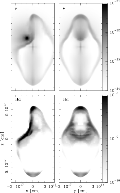
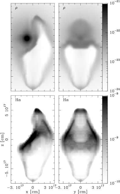
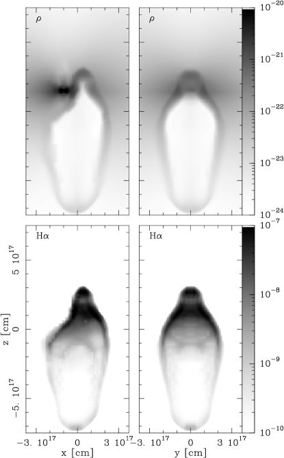
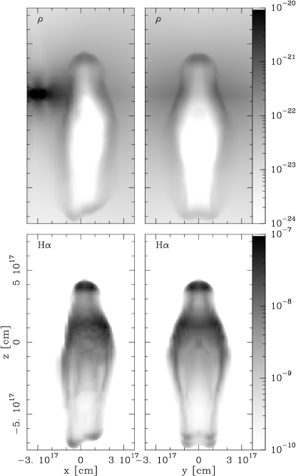
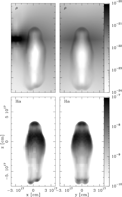
In Figures 2-6, we show some of the results obtained from models M1-M5 for the times $t_{f}$ (see Table 1) at which the shell which is pushed out by the bipolar “pulse” reaches one of the boundaries of the computational domain. These Figures show the density stratifications on the $xz$-plane (which includes the positions of both the wind and the “bipolar pulse” sources, see Figure 1) and on the $yz$-plane. These Figures also show the H$\alpha$ maps obtained by integrating the H$\alpha$ emission coefficient (including the radiative recombination cascade and the $n=1\to 3$ collisional excitations) along the $y$- and $x$-axes.

The models with spherically symmetric winds (models M1 and M2, Table 1) produce highly asymmetric $xz$-plane density stratifications and $xz$-H$\alpha$ emission maps (left hand side frames of Figures 2 and 3). The upper lobe of the shell (which is pushed out by the bipolar pulse) shows a major “indentation” formed by the interaction with the dense region at the base of the stellar wind. The $yz$-plane cuts and H$\alpha$ maps (right hand side frames of Figures 2 and 3) show an upper lobe which is narrower and shorter than the bottom lobe, with a larger asymmetry for the model with larger mass loss rate (model M2, see table 1).

In model M3, we have a wind mass loss rate intermediate between the ones of models M1 and M2 (see Table 1), but we have considered a latitude-dependent wind (with $\xi=20$ and $p=0.5$, see equation 3). In model M3 (see Figure 4), the bottom lobe of the outflow is somewhat narrower, but otherwise similar to the corresponding lobes of models M1 and M2 (see Figures 2 and 3). The upper lobe of model M3, however, is strongly reduced in size, leading to a large asymmetry between the top and bottom lobes of the expanding shell.

In models M4 and M5, we have moved the stellar wind source away from the axis of the “bipolar pulse” ejection (see Table 1 and Figures 5 and 6). These models have a high, ${\dot{M}}_{w}=10^{-5}$M_⊙yr^-1 mass loss rate and two different degrees of asymmetry ($\xi=20$ and 50 for models M4 and M5, respectively). These models produce top-to-bottom lobe asymmetries which are qualitatively similar to the ones obtained from model M3 (see above and Figure 4).

As can be seen from the left hand side plots of Figures 5 and 6, models M4 and M5 have the interesting property that the side-to-side asymmetries of the top lobe (when seen in the $xz$-plane density cut or H$\alpha$ map) are much less important than the ones found in models M1-M3. This result indicates that a wind with a strong latitude dependence from a source placed well away from the axis of the “bipolar pulse” produces a strong asymmetry between the two lobes of the expanding shell, but does not introduce strong deviations from the initial axisymmetry of the bipolar pulse.

Models M4 and M5 show a double peak structure at the bottom lobe (see Figures 5 and 6), which are reminiscent of the results obtained from numerical simulations of stellar jets for a high jet to environment density ratio (e.g., Raga 1988; Downes & Cabrit 2003).

0.4 Discussion

The results of our 3D numerical simulations of the interaction between a bipolar “pulse” and a continous wind ejected by a companion star indicate that the overall morphology (particularly, the strong differences between the sizes and velocities of the two lobes) of the PPN OH231.8+4.2 can be modeled as the result of such an interaction.

We have adopted a bipolar “pulse” (described by equations 5, 6, 7, and 8) instead of a continous jet, as an outflow of this kind appears to be implied by the observed Hubble-like velocity law (see §1). Also, we have taken the parameters ($\rho_{c}$, $v_{c}$, and $\theta_{c}$), of the dense, high-velocity jet (see §2.3) that would be necessary for explaining the CO observations of OH 231.8+4.2 of Alcolea et al. (2001).

The parameters describing the wind from the companion star (i.e., QX Pup in the case of OH 231.8+4.2) are the wind velocity ($v_{w}$) and the mass loss rate ($\dot{M}_{w}$). We have adopted a value of 40 km s^-1 for the wind velocity, which corresponds to the escape velocity from QX Pup (Alcolea 2004) and mass loss rate values characteristic of Mira variables (with values ranging from 10^-6 to 10^-5 $M_{\odot}$ yr^-1; see Table 1). We have considered a stellar wind with a latitude dependent density, with a density enhancement at the equator. The equator is perpendicular to the “bipolar pulse”, as suggested by the spatial distribution of the SiO maser associated with QX Pup (Sánchez Contreras et al. 2002).

With these parameters we have computed several numerical simulations, from which we have obtained the H$\alpha$ emission maps, that can be compared with the H$\alpha$ images of OH 231.8+4.2 (Sánchez Contreras et al. 2000a; Bujarrabal et al. 2002).

The numerical simulations reproduce qualitatively well several characteristics of the H$\alpha$ image of OH 231.8+4.2. The observed and predicted H$\alpha$ maps have bipolar structures with strong lobe-to-lobe asymmetries. We should point out that the hourglass morphology of OH 231.8+4.2 is not reproduced by these models. This discrepancy can be solved by including a dense disk (or torus) around the central source (as has been shown numerically by several authors; see, e.g., Frank & Mellema 1996). However, we have not included such a torus in the present simulations.

All of our models show an upper lobe which is narrower and shorter than the bottom lobe, but the large asymmetry between the Northern and Southern lobes of OH 231.8+4.2 is only reproduced by the models with a latitude dependent wind (M3 - M5). Figures 4, 5 and 6 illustrate that the upper lobe is strongly reduced in size in the latitude-dependent wind models, and that the ratio of $\sim 2$ between the sizes of the two lobes is in qualitative agreement with the observations of OH 231.8+4.2 (Bujarrabal et al. 2002). However, the width of the Southern lobe is better predicted by the models with spherically symmetric winds (models M1 and M2).

Figure 7: Results obtained for model M3 for a $t_{f}=1500$ yr (see the text and table 1). The left and middle frames show the velocity field on the xz-plane (left) and yz-plane (middle). The velocity maps (arrows) are superposed on the density stratification, with linearly spaced isolines with steps of 5 x 10^-22 g cm^-3. The right frame shows the axial velocity along the symmetry axis.

To illustrate the predicted velocity field, we present the velocity field of model M3 on the xz-plane and yz-plane (see Figure 7). For a comparison with the observed properties we also present the axial velocity along the symmetry axis (see Figure7). The predicted kinematics reproduces the strong velocity gradient observed along the nebular axis (Alcolea et al. 2001; Sánchez Contreras et al. 2000). However, we find that the model prediction gives velocities lower than the observed ones (by a factor of 3 to 4). In the top lobe, the model produces a too sharp drop in the velocity. In order to obtain a better agreement with the observations, we would need to have a model with a higher velocity bipolar pulse.

We have presented a number of 3D simulations of a bipolar pulse interacting with a continuos wind ejected by a close companion star. In our simulations, we have used a dense, AGB wind with mass loss rates typical of AGB stars. We have shown that the strong asymmetries between both lobes of this nebula can indeed be explained in terms of a the proposed bipolar pulse/continous wind interaction model (the companion star ejecting the wind has to be located within the Northern lobe). We find that the observed lobe-to-lobe asymmetry can be explained without invoking an intrinsic asymmetry in the ejection of the jet and the counterjet.