Colors, magnitudes and velocity dispersions in early-type galaxies: Implications for galaxy ages and metallicities

Abstract

We present an analysis of the color-magnitude-velocity dispersion relation for a sample of 39320 early-type galaxies within the Sloan Digital Sky Survey. We demonstrate that the color-magnitude relation is entirely a consequence of the fact that both the luminosities and colors of these galaxies are correlated with stellar velocity dispersions. Previous studies of the color-magnitude relation over a range of redshifts suggest that the luminosity of an early-type galaxy is an indicator of its metallicity, whereas residuals in color from the relation are indicators of the luminosity-weighted age of its stars. We show that this, when combined with our finding that velocity dispersion plays a crucial role, has a number of interesting implications. First, galaxies with large velocity dispersions tend to be older (i.e., they scatter redward of the color-magnitude relation). Similarly, galaxies with large dynamical mass estimates also tend to be older. In addition, at fixed luminosity, galaxies which are smaller, or have larger velocity dispersions, or are more massive, tend to be older. Second, models in which galaxies with the largest velocity dispersions are also the most metal poor are difficult to reconcile with our data. However, at fixed velocity dispersion, galaxies have a range of ages and metallicities: the older galaxies have smaller metallicities, and vice-versa. Finally, a plot of velocity dispersion versus luminosity can be used as an age indicator: lines of constant age run parallel to the correlation between velocity dispersion and luminosity.

1. Introduction

It has long been known that early-type galaxies tend to be the reddest galaxies, and that the more luminous the galaxy, the redder its color (e.g. Sandage & Viswanathan 1978a,b; Bower, Lucey & Ellis 1992a,b). The tightness of the correlation between color and magnitude has been used to constrain models of how early-type galaxies formed. However, a luminous galaxy may appear red either because its stars are older, or because, although its stars are younger, they are more metal rich. This has complicated the constraints one can place on galaxy formation models: should the models produce luminous metal-rich galaxies, or luminous old galaxies? To illustrate, Appendix A shows the color-magnitude relation associated with the recent stellar population synthesis models of Bruzual & Charlot (2003).

The colors and luminosities of older galaxies are expected to evolve more slowly than those of younger ones. Therefore, if age is changing along the color-magnitude sequence (e.g. if the more luminous galaxies are older), one would expect the differential evolution of the older and younger populations along the sequence to manifest as a change in the slope of the color-magnitude relation with redshift. Recent measurements have shown that the relation was already in place at redshifts of order unity, and that its slope appears to be unchanged from its value locally (e.g. Kodama et al. 1998; Blakeslee et al. 2003). If the high redshift population does indeed represent the local low redshift population in its youth, then the fact that the slope has evolved little argues against a large age-spread along the relation. In this case, the color-magnitude relation is caused primarily by a correlation between metallicity and luminosity (Kodama et al. 1998). (This argument becomes weaker if the redshift at which the population formed the bulk of its stars is large.)

In this framework, the scatter around the color-magnitude relation is usually attributed to the effects of age. It is not entirely obvious, however, that this can be correct. This is because differential evolution must make the scatter around the mean relation larger at higher lookback times. Therefore, the fact that the color-magnitude relation is well defined at redshifts of order unity can be translated into a constraint on the mix of ages present at redshift zero. For this reason, it would be interesting to quantify how the scatter around the mean relation evolves. (Blakeslee et al. 2003 find little evolution in the slope and scatter of the relation, using cluster early-types out to redshifts of order unity.)

It is well known that luminosity also correlates with velocity dispersion (Poveda 1961; Faber & Jackson 1976), so it is natural to ask if velocity dispersion is also tightly coupled to metallicity. The tightness of the correlation between Mg₂ and $\sigma$ (e.g. Bernardi et al. 1998; Colless et al. 1999), is thought to be a consequence of variations in age and metallicity which conspire to keep the observed correlation tight (e.g. Kuntschner et al. 2001). In this view, old galaxies with a given $\sigma$ tend to be metal poor, whereas younger galaxies with the same $\sigma$ are metal rich (e.g. Worthey 1994; Trager et al. 2000b).

Thus, recent work suggests that residuals from the color-magnitude relation are age indicators, whereas studies of chemical abundances suggest that velocity dispersion is a combination of both age and metallicity. One of the goals of the present work is to see if these conclusions are consistent with one-another. We do this by studying the joint distribution of color, luminosity and velocity dispersion in a sample of 39320 early-type galaxies drawn from the Sloan Digital Sky Survey (York et al. 2000; Stoughton et al. 2002; Abazajian et al. 2003) database (hereafter SDSS).

Section 2 describes our sample. Section 3 presents the color-magnitude and color-$\sigma$ relations, and demonstrates that color-$\sigma$ and magnitude-$\sigma$ are the primary correlations. A simple model is introduced which illustrates clearly what our measurements imply for the relations between age, metallicity and velocity dispersion. The mathematics associated with this model is in Appendix B. Section 4 uses the model to derive a number of consequences of the observed color-magnitude-$\sigma$ relations, and summarizes our findings.

Throughout, we assume that $H_{0}=70$ km s^-1 Mpc^-1 in a universe with $\Omega_{0}=0.3$ which is spatially flat.

Figure 1.— Luminosity correlates with both velocity dispersion (bottom) and size (middle), but the tightest correlation is with $R_{r}\sigma^{2}\propto$ mass (top). Dashed lines show the correlations summarized in Table 1. Luminosities have been corrected for evolution by 0.85$z$ (see text for details).

2. The SDSS early-type galaxy sample

For our analysis we used galaxies selected from the Sloan Digital Sky Survey (SDSS) database. See York et al. (2000) for a technical summary of the SDSS project; Stoughton et al. (2002) for a description of the Early Data Release; Abazajian et al. (2003) et al. for a description of DR1, the First Data Release; Gunn et al. (1998) for details about the camera; Fukugita et al. (1996), Hogg et al. (2001) and Smith et al. (2002) for details of the photometric system and calibration; Lupton et al. (2001) for a discussion of the photometric data reduction pipeline; Pier et al. (2003) for the astrometric calibrations; Blanton et al. (2003) for details of the tiling algorithm; Strauss et al. (2002) and Eisenstein et al. (2001) for details of the target selection.

Table 1Maximum-likelihood estimates, in the SDSS $r$ band, of the joint distribution of luminosities, sizes and velocity dispersions. The mean values of the variables at redshift $z$, $M_{*}-Qz$, $R_{*}$, $V_{*}$, and the coefficients of the various pairwise correlations between the variables are shown. The coefficient which differs most from Table 1 of Bernardi et al. (2003b) is $R_{*}$.

Band	$M_{*}$	$\sigma_{MM}$	$R_{*}$	$\sigma_{RR}$	$V_{*}$	$\sigma_{VV}$	$\xi_{RM}$	$\xi_{VM}$	$\xi_{RV}$	Q
$r$	$-21.025$	0.841	0.354	0.263	2.220	0.111	$-0.900$	$-0.774$	0.550	0.85

Our early-type galaxy sample is selected similarly to that of Bernardi et al. (2003a), with some minor changes: We selected all objects targeted as galaxies and having de-reddened Petrosian apparent magnitude $14.5\leq r_{\rm Pet}\leq 17.75$. To extract a sample of early-type galaxies we then chose the subset with the spectroscopic parameter eclass < 0 (eclass classifies the spectral type based on a Principal Component Analysis), and the photometric parameter fracDev_r > 0.8. (The parameter fracDev is a seeing-corrected indicator of morphology. It is obtained by taking the best fit exponential and de Vaucouleurs fits to the surface brightness profile, finding the linear combination of the two that best-fits the image, and storing the fraction contributed by the de Vaucouleurs fit.) We removed galaxies with problems in the spectra (using the zStatus and zWarning flags). From this subsample, we finally chose those objects for which the spectroscopic pipeline had measured velocity dispersions (meaning that the signal-to-noise ratio in pixels between the restframe wavelengths 4200Å and 5800Å is S/N $>10$). These selection criteria produced a sample of 39320 objects with photometric parameters output by version ${\tt V5.4}$ of the SDSS photometric pipeline and ${\tt V.23}$ reductions of the spectroscopic pipeline (i.e. ${\tt v4\_10\_2}$ of ${\tt idlspec2d}$ and ${\tt v5\_9\_4}$ of ${\tt spectro1d}$).

The main quantities we use in this paper are magnitudes, sizes, colors, redshifts and velocity dispersions; the first three are output from the SDSS photometric pipeline, and the final two from the SDSS spectroscopic pipeline. The photometry is accurate to 0.02 mags, and the velocity dispersions to about $8$% (see Bernardi et al. 2003a). We work with de Vaucouleurs (1948) magnitudes and sizes, and SDSS model colors throughout: these are colors measured within an aperture which scales with the de Vaucouleurs half-light radius in the $r$-band.

Figure 2.— Color-magnitude relation in the sample. Top series of panels show the raw measurement, and bottom panels show the result of making magnitudes fainter by $0.85z$ mag and colors redder by $0.3z$ mag to account for evolution. Both on the top and bottom, the left-most panel shows the color-magnitude relation in the full sample, and the other two panels show the relation in small bins in velocity dispersion. Clearly, at fixed velocity dispersion, there is no relation between color and magnitude.

The most important reason for analyzing a new sample (other than size) is that the old photometric reductions output by the SDSS pipeline photo were incorrect (see documentation on DR2, the Second Data Release). A comparison of the properties of objects for which old and new photometric reductions are available shows that the new corrected photometry has made most magnitudes slightly fainter ($\sim 0.13$ mags), and most half-light radii smaller ($\sim$10%). It is customary to report velocity dispersions at some fraction (we use 1/8) of the half-light radius. The half-light radii of the galaxies which enter our sample are typically about 2 arcsecs, approximately independent of redshift, whereas the SDSS fiber used to measure the spectrum from which the velocity dispersion is estimated has a diameter of 3 arcsec. Since the velocity dispersions of early-type galaxies are known to increase towards the center (following Jørgensen et al. 1995 we assume the scaling is $\propto(r/r_{e})^{0.04}$, where $r_{e}$ is the half-light radius), all measured velocity dispersions are ‘aperture corrected’, and it is these which are usually reported (the mean correction is 7%). Although the measured velocity dispersions have not changed, the new photometry has changed the half-light radius. Hence, aperture corrected velocity dispersions differ from those associated with the old photometry (i.e., those reported in Bernardi et al. 2003a) by less than one percent (the new values are larger by a factor of $1.1^{0.04}$).

Table 2Maximum-likelihood estimates of the joint distribution of color, $r$-band magnitude and velocity dispersion and its evolution. At redshift $z$, the mean values are $C_{*}-Pz$, and the covariances are $\langle(C-C_{*})(M-M_{*})\rangle=\sigma_{CC}\sigma_{MM}\,\xi_{CM}$, and similarly for $\xi_{CV}$ ($M_{*}$ and $V_{*}$ are given in Table 1).

Color	$C_{*}$	$\sigma_{CC}$	$\xi_{CM}$	$\xi_{CV}$	$P$
$g-r$	0.736	0.057	$-0.361$	0.516	0.30

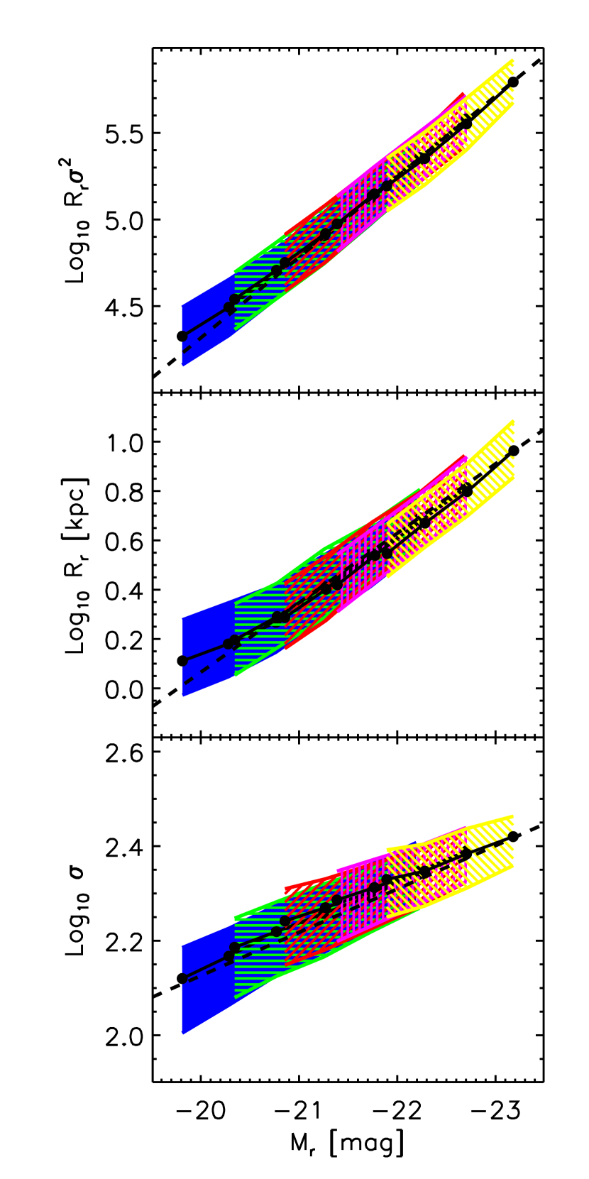
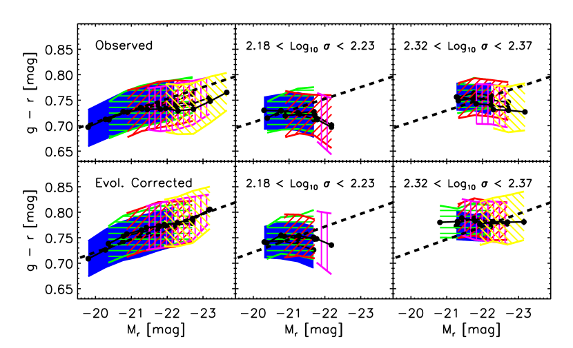
Bernardi et al. (2003b) showed that the luminosities in their sample ($\sim 9000$ galaxies with $z\leq 0.3$) evolve: $M_{*}(z)=M_{*}(0)-0.85z$, where $M_{*}(z)$ denotes the mean absolute magnitude at redshift $z$. We find similar evolution in the new sample: the main difference is that the new photometric reductions make $M_{*}$ fainter by about 0.125 mags. The evolution is consistent with that of a passively aging population. Thus, in the analysis which follows, we will be careful to separate trends with redshift that are due to the magnitude limit of the sample, from trends that are due to evolution. Many of the following figures present measurements made in a series of narrow redshift bins: $0.02\leq z<0.07$, $0.07\leq z<0.09$, $0.09\leq z<0.12$, $0.12\leq z<0.15$, and $0.15\leq z<0.2$. In all of these figures, symbols show the median value of the variable on the y-axis as a function of the observable on the x-axis, error bars show the rms error of the median, and hashed regions indicate where the central 68% of the sample in each redshift bin lies.

Figure 1 displays correlations between luminosity, size $R_{r}$, and velocity dispersion $\sigma$ in this sample. (The half-light radius in kpc, $R_{r}$, is defined similarly to the quantity called $R_{o}$ by Bernardi et al. 2003a, for the $r$-band.) The dashed lines show fits to these correlations, summarized in Table 1. In all cases, luminosities have been corrected for evolution by 0.85$z$. In the Table, $M_{*}$ and $\sigma_{M}$ are the mean and rms values of a Gaussian fit to the evolution-corrected $r$-band luminosity function, $Q$ quantifies the rate of luminosity evolution, and $R_{*}$ and $V_{*}$ are the values of $\log_{10}$(size/$h^{-1}$kpc) and $\log_{10}$(velocity dispersion/km s^-1) for an $L_{*}$ galaxy. In general, these values are all qualitatively similar to those reported in Bernardi et al. (2003b), but there are quantitative differences, most noticably in the mean size $R_{*}$, which is smaller by about ten percent. Table 1 also reports values of a number of pairwise correlations in the following format. Given a pair of observables $X$ and $Y$, $\langle Y-Y_{*}|X\rangle/\sigma_{YY}=\xi_{XY}(X-X_{*})/\sigma_{XX}$. The results of a similar analysis of the correlations between color, magnitude and velocity dispersion is given in Table 2.

3. Color-magnitude and color-$\sigma$ relations

Figure 2 shows the color-magnitude relation in our sample. The top series of panels shows the raw measurement, and bottom panels show the result of accounting for evolution by adding $0.85z$ mags to the magnitudes, and adding $0.3z$ mags to the colors (see Table 2). On both tiers, the left-most panel shows the color-magnitude relation in the full sample, and the other two panels show the relation in small bins in velocity dispersion. The figure makes two important points: (i) at fixed velocity dispersion, there is no relation between color and magnitude, and (ii) the slope of the relation in the leftmost panel is approximately the same in all redshift bins.

We also find no evidence that the scatter around the mean relations changes with redshift, but placing a precise limit of the evolution is difficult, because the expected signal is small, so the answer is sensitive to uncertainties in the SDSS photometry (0.02 mags) and the $k$-correction. Specifically, because we $k$-correct following the procedure described in Bernardi et al. (2003a), all galaxies at the same redshift are assigned the same $k$-correction. This leads to a small amount of scatter (less than 0.02 mags) in our absolute magnitudes and colors which may well depend on redshift.

Figure 3 shows the color-$\sigma$ relation in the sample. The format is the same as for the previous figure: top panels show the raw measurement, and bottom panels show the result of accounting for evolution by adding $0.3z$ mags to the colors, as was required to model the evolution of the color magnitude relation. The left-most panels show the color-$\sigma$ relation in the full sample, and the other two panels show the relation for galaxies which are restricted to a narrow range in magnitude. Clearly, at fixed redshift, the correlation between color and $\sigma$ is the same for all magnitude bins.

Comparison of the color-$\sigma$ relation in the different redshift bins suggests that the relation is steepening slightly with redshift: galaxies with small velocity dispersions are evolving slightly more rapidly. Because we are no longer making measurements at fixed magnitude, one may wonder if the slope of the color-$\sigma$ relation is affected by the magnitude-limited selection. Appendix B develops a simple model which demonstrates that this is not the case. We have also checked that the slope change does not depend strongly on our choice of $k$-correction. With the current sample size, this steeping is barely significant: it will be interesting to see if this steepening persists when the sample is larger.

Figure 3.— Color-$\sigma$ relation in the sample. Top series of panels show the raw measurement, and bottom panels show the result of accounting for evolution by adding $0.3z$ mags to the colors, as was required to model the evolution of the color magnitude relation. Both on the top and bottom, the left-most panel shows the color-$\sigma$ relation in the full sample, and the other two panels show the relation in small bins in magnitude. Clearly, at fixed redshift, the correlation between color and $\sigma$ is the same, whatever the magnitude.

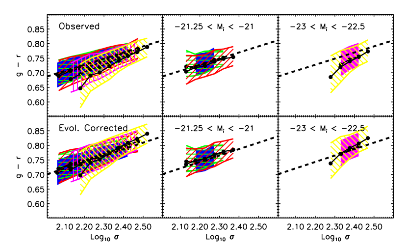
Together, Figures 2 and 3 indicate that the color-magnitude relation is entirely a consequence of the color-$\sigma$ and magnitude-$\sigma$ relations. In particular, the joint distribution of color, magnitude and velocity dispersion is:

$$p({\rm color},{\rm mag},\sigma)=p(\sigma)\,p({\rm mag}|\sigma)\,p({\rm color}|\sigma).$$ (1)

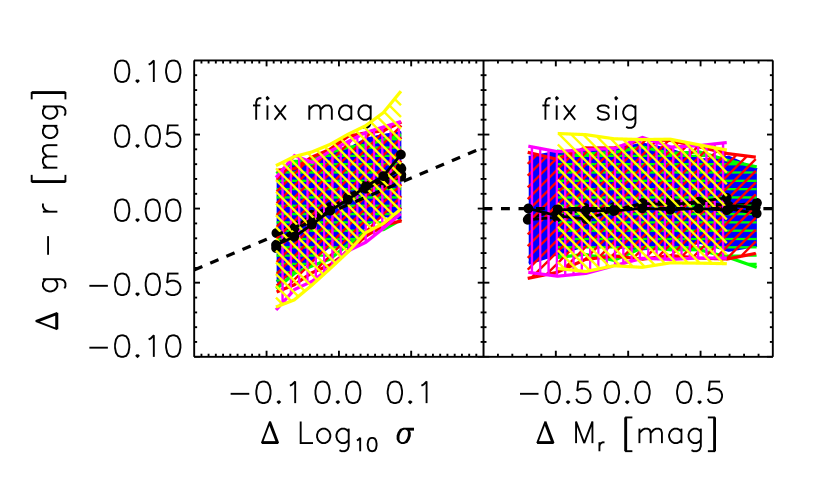
Appendix B demonstrates that if this expression is correct, then residuals from the magnitude-$\sigma$ relation should not correlate with residuals from the color-$\sigma$ relation. This is shown in Figure 4: $M-\langle M|\sigma\rangle$ does not correlate with ${\rm color}-\langle{\rm color}|\sigma\rangle$, but $\sigma-\langle\sigma|M\rangle$ does correlate with ${\rm color}-\langle{\rm color}|M\rangle$. Moreover, residuals from the color-$\sigma$ relation should not correlate with magnitude, whereas residuals from the color-magnitude relation should correlate with velocity dispersion. The two panels in Figure 5 show that this is indeed the case. Note that the slope of the correlation between ${\rm color}-\langle{\rm color}|M\rangle$ and $\sigma$ is not as steep as for the color-$\sigma$ relation itself. In effect, this is because $\langle{\rm color}|M\rangle$ correlates with $\sigma$ (because $M$ itself correlates with $\sigma$).

The bottom panel of Figure 5 shows that the correlation between color-magnitude residuals (i.e., age) and velocity dispersion steepens systematically with redshift. Although it is tempting to conclude that this is evidence of differential evolution, the analysis in Appendix B shows that it is, in fact, a selection effect (see text between equations B9 and B10).

Figure 4.— Residuals from the color-magnitude relation correlate with residuals from the $\sigma$-magnitude relation (left) whereas residuals from the color-$\sigma$ relations do not correlate with residuals from the magnitude-$\sigma$ relation (right). Dashed lines show the relations from our model, equation (B1), obtained by inserting the values from Tables 1 and 2 in equations (B7) and (B6), respectively.

4. Interpretation and discussion

Suppose that the color-magnitude relation is a consequence of the fact that metallicity increases with luminosity along the sequence, and that the galaxies which scatter redward of the relation are older. Then the correlation in Figure 5 suggests that galaxies with large velocity dispersions are, on average, older.

Figure 5.— Residuals from the color-$\sigma$ relations do not correlate with magnitude (upper panel), whereas residuals from the color-magnitude relation do correlate with velocity dispersion (bottom panel). Dashed lines show the relations from our model, equation (B1), obtained by inserting the values from Tables 1 and 2 in equations (B12) and (B9), respectively. The bottom panel can be interpreted as showing that galaxies with large velocity dispersions tend to have older stellar populations. Although the steepening at higher redshifts in the bottom panel suggests that the scatter around the mean color-magnitude relation is larger at high redshift, or that evolution is differential, it is, in fact, a selection effect (see text between equations B9 and B10).

Figure 6.— Galaxies which scatter blueward of the color-magnitude relation scatter towards smaller masses from the mass-luminosty relation (top). At fixed mass, redder galaxies tend to be fainter (second), have smaller sizes (third), and have larger velocity dispersions (bottom). Since mass $\propto R_{r}\sigma^{2}$, the trend with $\sigma$ shown in the bottom panel could have been inferred directly from the trend with size.

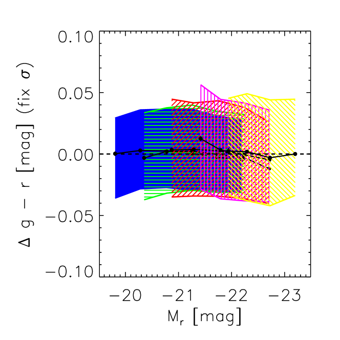
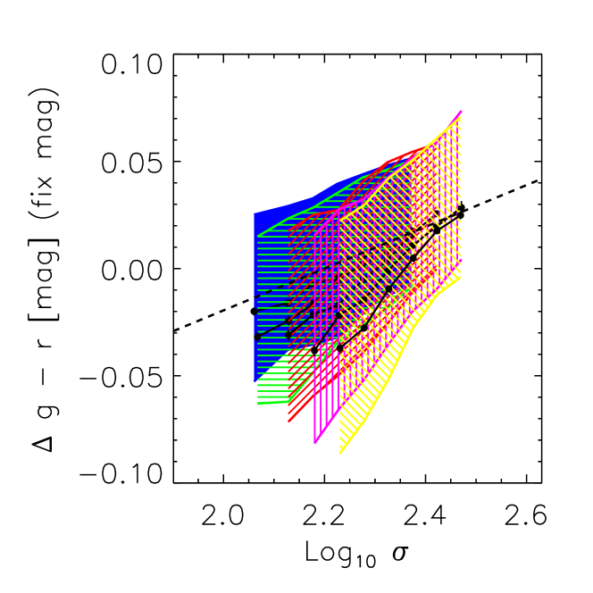
The correlation in the panel on the left of Figure 4 implies that older galaxies tend to have larger velocity dispersions than their luminosities indicate. A correlation between age and the residuals from the $\sigma$-luminosity relation was found by Forbes & Ponman (1999), but their age estimates came from comparing the spectra of these objects with stellar population synthesis models. Our analysis indicates that age estimates from the color-magnitude relation lead to the same conclusion. (Note that the analysis in Appendix B suggests that age is more closely related to the residuals in $\sigma$ with respect to the mean $\langle\sigma|L\rangle$ relation, than to the residuals in magnitude with respect to the $\langle L|\sigma\rangle$ relation. That is, the residuals studied by Forbes & Ponman (1999) should be more closely related to age than those studied more recently by Proctor et al. 2004.)

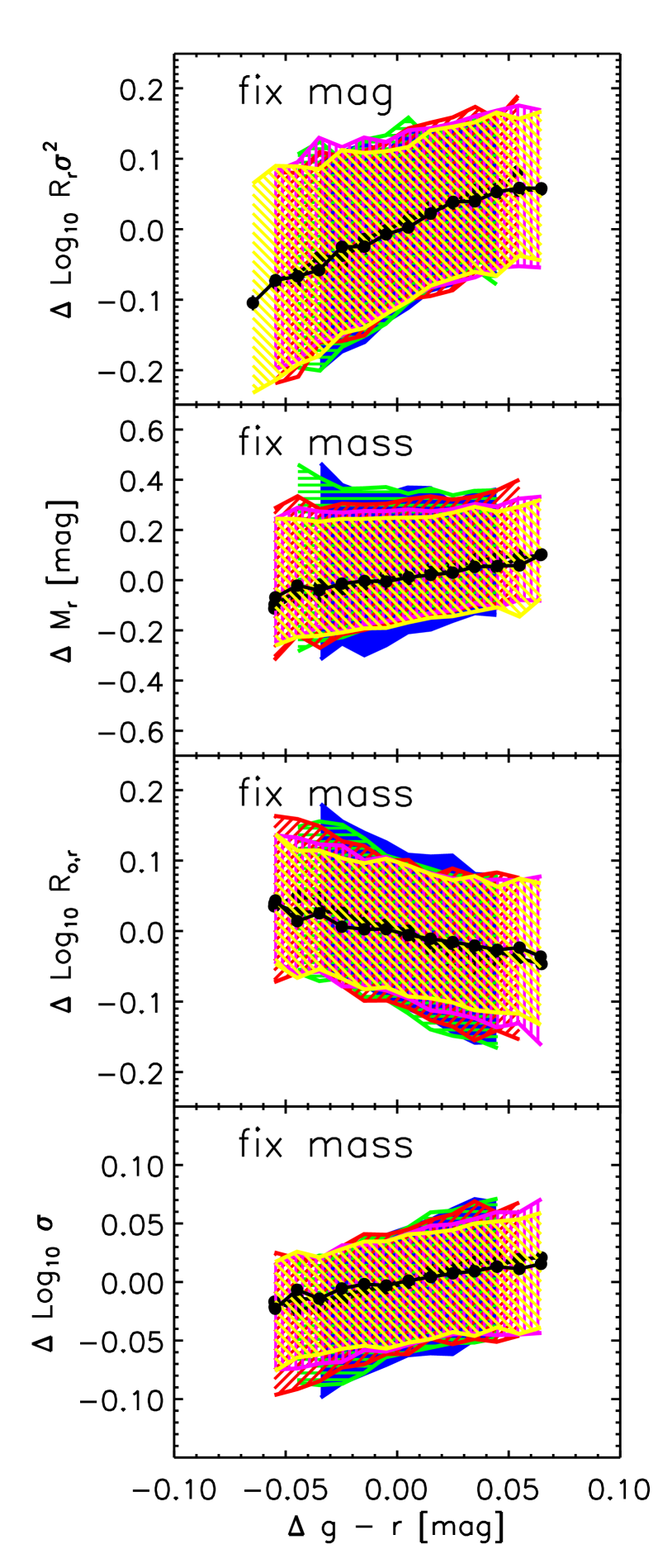
Figure 1 shows that luminosity is tightly correlated with mass $\propto R_{r}\sigma^{2}$. So it is interesting to study how residuals from the color-magnitude relation correlate with residuals from the mass-luminosity relation. The top-most panel of Figure 6 shows that galaxies which scatter blueward from the color-magnitude relation tend to scatter to smaller masses from the mass-luminosity relation. The other panels show that, at fixed mass, redder galaxies tend to be fainter (second from top), have smaller sizes (third from top), and have larger velocity dispersions (bottom). Since luminosity and mass are so tightly correlated, we can think of the color-mass residual as being similar to the color-magnitude residual. If we treat the color-magnitude residual as an age indicator, then Figure 6 indicates that, at fixed mass, older (redder) galaxies are fainter, smaller, and have larger velocity dispersions. All of these trends are qualitatively similar to those of dark matter halos, but they are also consistent with a model in which the bluer light is less concentrated than the red light (see, e.g. Figure 3 in Bernardi et al. 2003a), as color gradients also suggest (e.g. Figure 7 in Bernardi et al. 2003d). Figure 7 is similar, but now the color-magnitude residual is shown as the dependent parameter.

Figure 7.— Similar to previous Figure, but now with color-magnitude residual as the dependent parameter.

In Figures 6 and 7, the first two panels from the top and left deserve further comment. The first panel indicates that bluer, lower mass galaxies can have the same luminosity as redder, more massive galaxies. This is easy to understand if the color deviation traces age. Suppose, instead, we wanted to construct a model in which the residuals from the color-magnitude relation trace metallicity rather than age, the redder galaxies being the more metal rich. In this case, one would interpret the first panel as indicating that lower mass, metal poor galaxies can have the same luminosity as more massive, metal rich galaxies. In the Bruzual-Charlot (2003) models, at fixed mass, color changes are associated with larger magnitude changes if the color change is tied to age rather than metallicity (see top-left panel of Figure 1). The two possiblities differ by a factor of two, so, in principle, one might to be able to distinguish between them using the second panels in Figures 6 and 7. Figure 6 suggests that $\langle\Delta M|\Delta(g-r)\rangle\propto\Delta(g-r)$, and Figure 7 suggests $\langle\Delta(g-r)|\Delta M\rangle\propto\Delta M/10$. These observed relations are shallower than both models: shallower relations indicate that scatter is important, but this makes it difficult to determine which of the two possibilities is more accurate.

Appendix B develops in some detail the consequences of a model in which the assumptions that metallicity increases with luminosity along the color-magnitude relation, and that the residuals from the relation are indicators of age, are combined with our finding that the color-magnitude relation is determined by the color-$\sigma$ and magnitude-$\sigma$ relations. (The Appendix also shows that these conclusions are unchanged if we use the orthogonal rather than the direct fit, i.e., if we assume metallicity varies along the principal axis of the color-magnitude relation, and age varies perpendicular to this axis.) In such a model:

• metallicity and $\sigma$ are correlated (galaxies with large velocity dispersions tend to be more metal rich);

• age and $\sigma$ are correlated (galaxies with large velocity dispersions tend to be older);

• lines which run parallel to the mean $\sigma$-magnitude relation are approximately lines of constant age;

• in the plane of age along the $x$-axis and metallicity along the $y$-axis, lines of constant velocity dispersion slope down and to the right.

If $\sigma$ is indeed sensitive to age, one might wonder if the slope of the color-$\sigma$ correlation steepens with redshift. The SDSS is a relatively shallow, magnitude-limited survey; the median redshift in our sample is of order 0.1, so the sample is not ideal for quantifying trends with redshift. On the other hand, it offers a large number of galaxies ($\sim 30000$) with well-calibrated surface photometry and velocity dispersions, so we may reasonably expect to be able to detect a small signal. We are also aided by the fact that, of the three pairwise relations, color-magnitude, $\sigma$-magnitude, and color-$\sigma$, it is the color-magnitude relation which is a consequence of the other two (c.f. Figures 2 and 3; also see Bernardi et al. 2003d). Because the color-$\sigma$ relation is the fundamental correlation, selection effects associated with the magnitude limit of our sample are unimportant (see Appendix B for details). The bottom left panel of Figure 3 suggests that the slope of the color-$\sigma$ relation is steepening with redshift, but data from higher redshift and a better understanding of the appropriate $k+e$-corrections are required before we can claim to have measured this with confidence. Other tantalizing evidence of evolution comes from Figure 5: the correlation between color-magnitude residuals (i.e., age) and velocity dispersion steepens systematically with redshift. Although it is tempting to conclude that this is additional evidence of evolution, the analysis in Appendix B shows that it is, in fact, a selection effect.

Taken together, the findings itemized above indicate that our data require the existence of an age-metallicity degeneracy; this degeneracy is most noticable for galaxies which have the same velocity dispersion $\sigma$. In this respect, our findings are consistent with Figure 4 of Trager et al. (2000b). But our results are inconsistent with their conclusion that the most massive galaxies are less metal rich (see their Figure 6). Indeed, Figure 1 indicates that it would be difficult for single burst models to produce the observed color-magnitude relation if the more luminous galaxies were older but less metal rich. Our finding that older galaxies tend to have larger velocity dispersions than their luminosities indicate is qualitatively consistent with one of the conclusions of Forbes & Ponman (1999); this is encouraging because their age estimates come from a very different approach (detailed comparison of spectral features with stellar population synthesis models).

While it is tempting to calibrate the relation between color-magnitude residual and age, this would be model-dependent. For example, the Bruzual-Charlot models presented in Appendix A can be used to perform this calibration. But we are hesitant to take this path because the models do not include an important correlation between velocity dispersion and $\alpha$-element abundance ratios (Trager et al. 2000a; Thomas, Maraston & Bender 2003; Proctor et al. 2004).

In the model developed here, the scatter around the color-magnitude and the $\sigma$-magnitude relations should increase with lookback time. This can be tested with data from redshifts of order one-half to unity which will soon be available (e.g. the SDSS-2dF survey of luminous red galaxies at http://sdss2df.ncsa.uiuc.edu/).

MB thanks A. Connolly for support.

Funding for the creation and distribution of the SDSS Archive has been provided by the Alfred P. Sloan Foundation, the Participating Institutions, the National Aeronautics and Space Administration, the National Science Foundation, the U.S. Department of Energy, the Japanese Monbukagakusho, and the Max Planck Society. The SDSS Web site is http://www.sdss.org/.

The SDSS is managed by the Astrophysical Research Consortium (ARC) for the Participating Institutions. The Participating Institutions are The University of Chicago, Fermilab, the Institute for Advanced Study, the Japan Participation Group, The Johns Hopkins University, the Korean Scientist Group, Los Alamos National Laboratory, the Max-Planck-Institute for Astronomy (MPIA), the Max-Planck-Institute for Astrophysics (MPA), New Mexico State University, University of Pittsburgh, Princeton University, the United States Naval Observatory, and the University of Washington.

Appendix A A: Single-burst models

In the single-burst models of Bruzual & Charlot (2003), galaxy colors depend on both age and metallicity. For a population which is older than one Gyr, and has solar metallicity or greater, we have found that the color is quite well described by:

$$g-r = 0.7+0.25(T-9.5)+{0.15\over 0.40}\,Z\qquad{\rm if\ T>9.5}$$

$$g-r = 0.7+0.50(T-9.5)+{0.15\over 0.40}\,Z\qquad{\rm if\ T<9.5}$$

where $T=\log_{10}$(age/Gyr).

The four panels of Figure 1 provide different examples of the color-magnitude relation associated with these models. The top left panel shows the locus traced out in the color-magnitude plane by a single object of fixed mass as it ages. The two dotted lines which slope from top left to bottom right show lines of constant metallicity (higher metallicity is redder), and the approximately vertical lines which connect them show locii of constant age (older is fainter). This panel is relevant to results presented in Figures 6 and 7. It shows that, at fixed mass, color changes are associated with larger magnitude changes if the color change is tied to age rather than metallicity: $\Delta M\propto 5\,\Delta(g-r)$ if the color change is entirely due to age, whereas $\Delta M\propto(5/2)\,\Delta(g-r)$ if the color change is entirely due to metallicity.

Figure 1.— Correlation between color and magnitude in the single-burst models of Bruzual & Charlot (2003). Different panels show the result of assuming the various correlations between luminosity, age and metallicity that are discussed in the main text. The top right panel shows color magnitude relations in models which have metallicity varying with luminosity. The bottom right panel shows relations in which age increases with luminosity. Bottom left panel shows models in which age and metallicity vary with luminosity. In the top two panels, solid and dashed lines which connect dots trace locii of constant age = 15.25, 12.75, 10.25, 7.75 and 5.25 Gyrs, with the oldest being reddest.

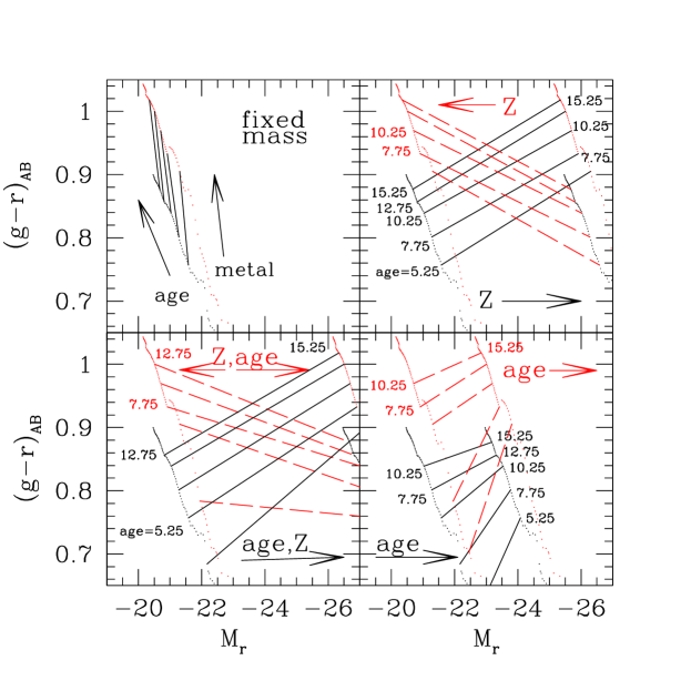
Top right panel shows models in which metallicity correlates with luminosity. The solid lines which span approximately the entire luminosity range show locii of constant age in a model which has metallicity increasing with luminosity. The dashed lines show constant age in a model where metallicity decreases with luminosity. Notice that, in both cases, the slope of the color magnitude relation is approximately independent of age. However, the data indicate that color increases with luminosity, so that models with metallicity decreasing with luminosity are not permitted.

The bottom right panel shows two models in which age, rather than metallicity, vary along the luminosity axis. Both models assume that older objects are more luminous, but the redder set of lines (i.e., the dashed lines) show a more metal rich population. In both cases, the slope of the relation varies more strongly with age than it did in the previous panel, with the slope of the color-magnitude relation evolving rapidly when the population is younger, but less rapidly at later times.

The two panels on the right showed models in which either metallicity or age varied with luminosity, but not both. Dashed lines which slope down and to the right in the bottom left panel show the color-magnitude relation in a model where the more luminous objects are older but metal poor. This model is qualitatively like those of Trager et al. (2000b). Solid lines show a model in which both age and metallicity increase with luminosity. The data are more consistent with this latter model which has more luminous objects being older and metal rich.

Appendix B B: Luminosities, colors, velocity dispersions, ages and metallicities

B.1. Luminosity, color and velocity dispersion

Define $m=(M-M_{*})/\sigma_{MM}$, $v=(V-V_{*})/\sigma_{VV}$, and $c=(C-C_{*})/\sigma_{CC}$, where $M$ is the absolute magnitude, $V\equiv\log_{10}$(velocity dispersion/km s^-1), and $C$ denotes a color. Our notation uses $X_{*}$ amd $\sigma_{XX}$ to denote the mean and rms of observable $X=M,V,C$, etc. This Appendix considers a model in which the only fundamental correlations are with $\sigma$:

$$p(v,m,c)=p(v)\,p(m|v)\,p(c|v).$$ (B1)

Pairwise correlations, such as that between luminosity and $\sigma$, are given by integrals like

$$\langle mv\rangle=\int dm\,dv\,dc\,(mv)\,p(v,m,c).$$ (B2)

For the assumed model, these are relatively simple to evaluate. If we suppose that the mean magnitude at fixed $\sigma$ scales as $\langle m|v\rangle=\xi_{mv}v$, and the mean color at fixed $\sigma$ is also linear in $v$, say $\xi_{cv}v$, then

$$\langle mv\rangle=\xi_{mv},\ {\rm and}\ \langle cv\rangle=\xi_{cv}.$$ (B3)

This comes from our choice to normalize $\langle vv\rangle=1$, and similarly for the other variables.

Let $\sigma_{m|v}$ denote the scatter in $m$ around $\langle m|v\rangle$. If $\sigma_{m|v}$ is independent of $v$, then

$$\langle v^{2}\rangle = \int dm\,p(m)\,\langle v^{2}|m\rangle$$ (B4)

$$= \int dm\,p(m)\,[\sigma_{v|m}^{2}+\xi_{vm}^{2}m^{2}]$$

$$= \sigma_{v|m}^{2}+\xi_{vm}^{2}$$

Therefore, $\sigma_{m|v}^{2}=1-\xi_{mv}^{2}$, and similarly for the scatter around the color-$\sigma$ relation.

What if we are interested in relations which do not involve $\sigma$? For instance, the mean color at fixed magnitude is

$$\langle c|m\rangle = \int dvdc\,c\,p(c|v)\,p(v|m)$$ (B5)

$$= \int dv\xi_{cv}v\,p(v|m)=\xi_{cv}\xi_{mv}\,m.$$

This shows that the slope of the color-magnitude relation can be written in terms of the slopes of the other two relations: $\xi_{cm}=\xi_{cv}\xi_{mv}$. This is a simple approximation to the observed correlations: $\xi_{cm}=-0.36$ and $\xi_{cv}\xi_{mv}=-0.40$ (from Tables 1 and 2).

By assumption (B1), the residuals of the $m$-$\sigma$ relation, $R_{m|v}=m-\langle m|v\rangle=m-\xi_{mv}v$, do not correlate with those of the color-$\sigma$ relation. It is straightforward to verify that this is so:

$$\langle R_{m|v}R_{c|v}\rangle = \langle(m-\xi_{mv}v)(c-\xi_{cv}v)\rangle$$ (B6)

$$= \langle mc-\xi_{cv}mv-\xi_{mv}vc+\xi_{mv}\xi_{cv}v^{2}\rangle$$

$$= 0.$$

However, the residuals of the color-magnitude relations do correlate with those of the $\sigma$-magnitude relation:

$$\langle R_{c|m}R_{v|m}\rangle \equiv \langle(c-\xi_{cm}m)(v-\xi_{vm}m)\rangle$$ (B7)

$$= \langle cv-\xi_{cm}mv-\xi_{vm}mc+\xi_{cm}\xi_{vm}m^{2}\rangle$$

$$= \xi_{cv}-\xi_{cm}\xi_{mv}=\xi_{cv}\,(1-\xi_{mv}^{2}).$$

Thus, this model explains the correlations between residuals shown in Figure 4.

Assumption (B1) has another important consequence. Namely, the slope of the color-$\sigma$ relation, at fixed magnitude, is

$$\langle c|v,m\rangle={\int dc\,c\,p(c|v)\,p(m|v)\,p(v)\over p(m,v)}=\xi_{cv}v.$$ (B8)

This shows that the slope of the $c$-$v$ correlation is the same as when the constraint on magnitudes is removed. Therefore, the slope of the color-$\sigma$ correlation measured in a magnitude limited sample is the same as the slope of the intrinsic relation. In other words, if the only correlation between color and magnitude is through $\sigma$, then the slope of the color-$\sigma$ relation measured in a magnitude limited sample is not biased by selection effects. We use this in the main text.

B.2. Age, metallicity and velocity dispersion

If the residuals from the color-magnitude relation, $R_{c|m}$, are indicators of age, and if the relation between age and $R_{c|m}$ is linear, then the mean age as a function of velocity dispersion can be obtained from

$$\langle R_{c|m}|v\rangle=(1-\xi_{mv}^{2})\,\xi_{cv}\,v.$$ (B9)

If $\xi_{cv}>0$, then age increases with increasing velocity dispersion. The rms scatter around this relation is $\sigma_{c|v}$. The bottom panel of Figure 5 shows this relation in the data. In this model, the mean age increases less rapidly with velocity dispersion (by a factor $1-\xi_{mv}^{2}$) than does the color, suggesting that some of the increase in color is associated with factors other than age.

In Figure 5, the relation between age and $\sigma$ appears to steepen with redshift. If real, what does this steepening imply? Note that the quantities in the Figure have not been normalized by their rms. If we suppose that the correlations between velocity dispersion, color, and magnitude do not evolve, but their rms values do, then the steepening implies that $(\sigma_{CC}/\sigma_{VV})$ is increasing. The distribution of velocity dispersions does not appear to be evolving (e.g. Sheth et al. 2003), and there are no strong reasons to expect it to. On the other hand, we argued in the Introduction that one expects to see the scatter around the color-magnitude relation increase with redshift. Although we do expect to see $\sigma_{CC}$ increase, the increase implied by Figure 5 is larger than expected. This is because the steepening is a selection effect—it is the result of the magnitude limit of the survey. To see why, note that the magnitude limit restricts the range in $m$ over which the integrals which define $\langle R_{c|m}|v\rangle=\int dm\,p(m|v)\,(\xi_{cv}v-\xi_{cm}m)$ are performed. If we write the result as $(1-\xi_{mv}^{2})\,\xi_{cv}v$ times a correction factor $\int dm\,p(m|v)\,(\xi_{cv}v-\xi_{cm}m)/(\xi_{cv}v-\xi_{cm}\xi_{mv}v)$, then this factor depends on the magnitude limit, so in effect, the slope of the correlation with $v$ depends on redshift.

Figure 1.— Correlations between residuals from the color-magnitude and color-$\sigma$ relations are well described by the model developed in the text. Dashed line in panel on the left shows the correlation described by equation (B10), and the line in the panel on the right shows equation (B11).

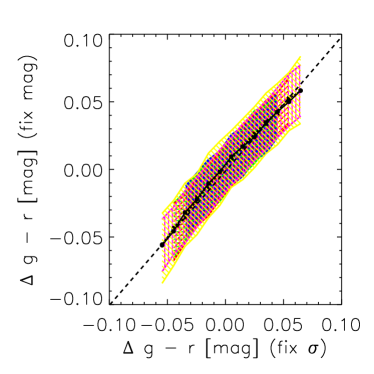
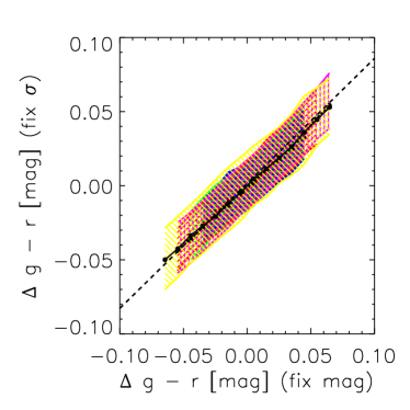
If the residuals from the color-$\sigma$ relation are a consequence of age and possibly other variables (such as metallicity and/or environment), then correlations between $R_{c|m}$ and $R_{c|v}$ can be used to study how much of the scatter in the color-$\sigma$ relation is due to age, and how much to other effects. For instance,

$$\langle R_{c|m}|R_{c|v}\rangle = R_{c|v},\quad{\rm and}$$ (B10)

$$\langle R_{c|v}|R_{c|m}\rangle = R_{c|m}\,{\sigma_{c|v}^{2}\over\sigma_{c|m}^{2}}=R_{c|m}\,{1-\xi_{cv}^{2}\over 1-\xi_{cv}^{2}\xi_{mv}^{2}}.$$ (B11)

This is consistent with the data has shown in Figure 1. Thus, although objects which have the same fixed offset in color from the color-$\sigma$ relation may have a range of ages, the mean age is the same as that infered from the color-offset of the color-magnitude diagram (see upper panel of Figure 1). On the other hand, the mean color offset from the color-$\sigma$ relation of objects which have the same age (i.e., they are all offset from the color-magnitude relation by the same amount) is smaller than the color-offset from the color-magnitude relation (see bottom panel of Figure 1). This is because some the color change associated with age effects has been accounted-for by the fact that age varies with $\sigma$.

In contrast, the result from Figure 5 (upper panel) showing

$$\langle R_{c|v}|m\rangle=0$$ (B12)

is less straightforward to interpret. This is because the previous correlations suggest that residuals from the color-$\sigma$ relation are some combination of both age and metallicity. If luminosity is driven primarily by metallicity, then the fact that $\langle R_{c|v}|m\rangle=0$ must mean that the age effects exactly cancel the correlation with metallicity. Moreover, if we replace luminosity with metallicity, then the fact that $\langle R_{c|m}|m\rangle=0$ suggests there is no correlation between age and metallicity.

The mean age at fixed luminosity and velocity dispersion is

$$\langle R_{c|m}|v,m\rangle=\xi_{cv}(v-\xi_{mv}m),$$ (B13)

and the rms scatter around this mean is $\sigma_{c|v}$. Since the final expression is really $\xi_{cv}\,R_{v|m}$, this shows that objects which have larger velocity dispersions than the mean $\sigma$-magnitude relation tend to scatter redward of the color-magnitude relation, and so are, on average, older than those which scatter to smaller dispersions. This has two important consequences. First, lines which run parallel to the mean $\langle v|m\rangle$ relation trace out curves of approximately constant age, and this statement becomes increasingly accurate if the relation between color and $\sigma$ is tight (recall that the scatter around $\langle R_{c|m}|v,m\rangle$ is $\sigma_{c|v}$). Second, if younger objects evolve more rapidly, and the evolution is stronger in luminosity than in velocity dispersion, then the scatter around the $\sigma$-magnitude relation should be larger at high redshift.

The mean velocity dispersion at fixed magnitude and color-magnitude residual is

$$\langle v|m,R_{c|m}\rangle=\xi_{mv}\,m+{\xi_{cv}(1-\xi_{mv}^{2})\over 1-\xi_{cm}^{2}}\,R_{c|m},$$ (B14)

with rms scatter $\sigma_{v|m}\sigma_{c|v}/\sigma_{c|m}$.

If age and metallicity scale as $T=aR_{c|m}$ and $Z=-bm$, with $a$ and $b$ both positive, then the same average value of $\sigma$ can be obtained by increasing the age and decreasing the metallicity, or vice-versa (we have assumed that $\xi_{mv}<0$, since, as Figure 1 shows, velocities tend to increase with luminosity). We have not discussed the roles played by the environment and by changes in $\alpha$-element abundances. In this model, they would be responsible for some of the scatter around these mean trends with age and metallicity.

The expression above suggests that different combinations of age and metallicity can yield the same average age. We can see this more directly by computing the correlation between age and metallicity at fixed velocity dispersion:

$$\langle mR_{c|m}|v\rangle-\langle m|v\rangle\langle R_{c|m}|v\rangle=-\xi_{cm}\sigma^{2}_{m|v}$$ (B15)

If age and metallicity scale as $T=aR_{c|m}$ and $Z=-bm$, with $a$ and $b$ both positive and $\xi_{cm}<0$, then the same value of $\sigma$ can be obtained by increasing the age and decreasing the metallicity, or vice-versa. This is also consistent with equation (B13): the mean age at fixed velocity dispersion increases as the metallicity decreases.

So far, we have not asked how one calibrates the relation between color-magnitude residual and age. In single burst models, it is possible to constrain the ratio $a/b$, because, at fixed $\sigma$, log₁₀(age) and metallicity are expected to be related by a factor of $-3/2$ (e.g. Worthey 1994).

In summary: We showed that the color-magnitude relation is determined by the color-$\sigma$ and magnitude-$\sigma$ relations. Previous work suggests that (i) metallicity increases with luminosity along the color-magnitude relation (as suggested by the observation that the slope of the color-magnitude relation does not evolve), and (ii) that the residuals from the relation are indicators of age. We developed a simple model which combines these results. The model implies that: (i) age and $\sigma$ are correlated (galaxies with large velocity dispersions tend to be older); (ii) lines which run parallel to the mean $\sigma$-magnitude relation are approximately lines of constant age; (iii) in the plane of age along the x-axis and metallicity along the y-axis, lines of constant velocity dispersion slope down and to the right; (iv) the scatter around the color-magnitude and the $\sigma$-magnitude relations should increase with lookback time.

B.3. The orthogonal fit

The previous section developed a model for correlations between age and $\sigma$ in which luminosity was proportional to metallicity, and residuals from the color-magnitude relation were proportional to log(age). Here, we change these assumptions slightly, and ask what happens if metallicity varies along the long axis of the color-magnitude relation, whereas age varies along the short axis. In this case, the age-metallicity plane is simply a rotation of the color-magnitude plane, so metallicity is some combination of luminosity and color, and age is some different combination. In particular, this would set

$$T\propto{\sigma_{c}c-a_{0}\sigma_{m}m\over\sqrt{1+a_{0}^{2}}}\quad{\rm and}\quad Z\propto-{a_{0}\sigma_{c}c+\sigma_{m}m\over\sqrt{1+a_{0}^{2}}},$$ (B16)

where

$$a_{0}={\sigma^{2}_{c}-\sigma_{m}^{2}\over 2\xi_{cm}\sigma_{c}\sigma_{m}}+\sqrt{1+\left({\sigma^{2}_{c}-\sigma_{m}^{2}\over 2\xi_{cm}\sigma_{c}\sigma_{m}}\right)^{2}}.$$

When $\sigma_{c}\ll\sigma_{m}$ then $a_{0}\to\xi_{cm}\sigma_{c}/\sigma_{m}$, the mean age $T$ at fixed velocity dispersion is $\propto\sigma_{c}(1-\xi_{mv}^{2})\,\xi_{cv}\,v$, and the mean value of $Z$ at fixed $v$ is $\propto-v\sigma_{m}\xi_{mv}(1+\xi_{cv}^{2}\sigma_{c}^{2}/\sigma_{m}^{2})/\sqrt{1+a_{0}^{2}}\to-v\sigma_{m}\xi_{mv}$. Thus, in this limit (because the luminosity in different bands is quite well correlated, the data do indeed have $\sigma_{c}\ll\sigma_{m}$), analysis of the orthogonal fit produces results which are similar to the analysis of the previous section.

If the scatter in colors were larger, the difference between the orthogonal fit model and the one studied in the previous subsection would also be larger. For instance, if $\sigma_{m}=\sigma_{c}$, then the age indicator would be $\propto(c-m)/\sqrt{2}$ and the metallicity would be $\propto(-c-m)/\sqrt{2}$, so the mean age at fixed velocity dispersion would be $\propto v\,(\xi_{cv}-\xi_{mv})/\sqrt{2}$, whereas the mean metallicity at fixed $v$ would scale as $-v\,(\xi_{cv}+\xi_{mv})/\sqrt{2}$. The rms scatter around the age-$\sigma$ and metallicity-$\sigma$ relations would be $\sqrt{(\sigma_{m|v}^{2}+\sigma_{c|v}^{2})/2}$. The mean correlation between age and metallicity at fixed $v$ is $(\xi_{cv}^{2}-\xi_{mv}^{2})/2$. In the sample, $\xi_{mv}<0$ and $|\xi_{mv}|>\xi_{cv}$, so the mean age and metallicity increase with velocity dispersion, and if the age is larger than expected for the velocity dispersion, then the metallicity is smaller. Moreover, the mean age would increase as luminosity increases: $(\xi_{cm}-1)\,m/\sqrt{2}=-m\,(1-\xi_{cv}\xi_{mv})/\sqrt{2}$, with rms scatter $\sigma_{c|m}$, and the mean metallicity would increase as $\langle Z|m\rangle=-m\,(1+\xi_{cv}\xi_{mv})/\sqrt{2}$, with the same rms scatter, $\sigma_{c|m}$. Although some of these conclusions are qualitatively similar to those of the previous subsection, they are generally quantitatively different: the correlations between age and velocity dispersion and age and luminosity become steeper, whereas those between metallicity and $\sigma$ and metallicity and luminosity become shallower.

References

- (1) Abazajian, K., et al. 2003, AJ, 126, 2081
- (2) Bernardi, M., Renzini, A., da Costa, L. N., Wegner, G., Alonso, M. V., Pellegrini, P. S., Rité, C. & Willmer, C. N. A. 1998, ApJL, 508, 143
- (3) Bernardi, M., Sheth, R. K., Annis, J., et al. 2003a, AJ, 125, 1817
- (4) Bernardi, M., Sheth, R. K., Annis, J., et al. 2003b, AJ, 125, 1849
- (5) Bernardi, M., Sheth, R. K., Annis, J., et al. 2003d, AJ, 125, 1882
- (6) Blakeslee, J. P., Franx, M., Postman, M. et al. 2003, ApJL, 596, 143
- (7) Blanton, M.R., Lupton, R.H., Maley, F.M., Young, N., Zehavi, I., & Loveday, J. 2003, AJ, 125, 2276
- (8) Bower, R. G., Lucey, J. R., & Ellis, R. S. 1992a, MNRAS, 254, 589
- (9) Bower, R. G., Lucey, J. R., & Ellis, R. S. 1992b, MNRAS, 254, 601
- (10) Bruzual, G., & Charlot, S. 2003, MNRAS, 344, 1000
- (11) Colless, M., Burstein, D., Davies, R. L., McMahan, R. K., Saglia, R. P., & Wegner, G. 1999, MNRAS, 303, 813
- (12) Connolly, A. J., & Szalay, A. S. 1999, AJ, 117, 2052
- (13) de Vaucouleurs, G. 1948, Annales d’Astrophysique, 11, 247
- (14) Eisenstein, D.J., Annis, J., Gunn, J.E., et al. 2001, AJ, 122, 2267
- (15) Fukugita, M., Ichikawa, T., Gunn, J.E., Doi, M., Shimasaku, K., & Schneider, D.P. 1996, AJ, 111, 1748
- (16) Faber, S. M., & Jackson, R. 1976, ApJ, 204, 668
- (17) Forbes, D. A., & Ponman, T. J. 1999, MNRAS, 309, 623
- (18) Gunn, J.E., Carr, M.A., Rockosi, C.M., Sekiguchi, M., et al. 1998, AJ, 116, 3040
- (19) Hogg, D.W., Schlegel, D.J., Finkbeiner, D.P., & Gunn, J.E. 2001, AJ, 122, 2129
- (20) Jørgensen, I., Franx, M. & Kjærgaard, P. 1995, MNRAS, 276, 1341
- (21) Kodama, T., Arimoto, N., Barger, A. J., & Arag’on-Salamanca, A. 1998, A&A, 334, 99
- (22) Kuntschner, H., Lucey, J. R., Smith, R. J., Hudson, M. J.ton, R., Gunn, J. E., Ivezić, Z., Knapp, G. R., Kent, S., & Yasuda, N. 2001, in ASP Conf. Ser. 238, Astronomical Data Analysis Software and Systems X, ed. F. R. Harnden, Jr., F. A. Primini, and H. E. Payne (San Francisco: Astr. Soc. Pac.), p. 269 (astro-ph/0101420)
- (23) Proctor, R. N., Forbes, D. A., Hau, G. K. T., Beasley, M. A., De Silva, G. M., Contreras, R., & Terlevich, A. I. 2004, MNRAS, 349, 1381
- (24) Pier, J.R., Munn, J.A., Hindsley, R.B., Hennessy, G.S., Kent, S.M., Lupton, R.H., & Ivezic, Z. 2003, AJ, 125, 1559
- (25) Poveda, A. 1961, ApJ, 134, 910
- (26) Sandage, A., & Visvanathan, N., 1978a, ApJ, 223, 707
- (27) Sandage, A., & Visvanathan, N., 1978b, ApJ, 225, 742
- (28) Sheth, R. K., Bernardi, M., Schechter, P. et al. 2003, ApJ, 594, 225
- (29) Smith, J.A., Tucker, D.L., Kent, S.M., et al. 2002, AJ, 123, 2121
- (30) Stoughton, C., Lupton, R.H., Bernardi, M., et al. 2002, AJ, 123, 485
- (31) Strauss, M.A., Weinberg, D.H., Lupton, R.H. et al. 2002, AJ, 124, 1810
- (32) Thomas, D., Maraston, C., & Bender, R. 2003, MNRAS, 339,897
- (33) Trager, S. C., Faber, S. M., Worthey, G., & González, J. J. 2000a, AJ, 119, 1645
- (34) Trager, S. C., Faber, S. M., Worthey, G., & González, J. J. 2000b, AJ, 120, 165
- (35) Worthey, G. 1994, ApJS, 95, 107
- (36) York, D.G., Adelman, J., Anderson, J.E., et al. 2000, AJ, 120, 1579