Constraints on the dark energy equation of state from recent supernova data
Abstract
Measurements suggest that our universe has a substantial dark energy component. The most recent data on type Ia supernovae give a dark energy density which is in good agreement with other measurements if the dark energy is assumed to be a cosmological constant. Here we examine to what extent that data can put constraints on a more general equation of state for the dark energy.
pacs:
98.80 -k, 98.80.EsI Introduction
It is generally believed, based on the analysis of type Ia supernovae red shift data hiz ; super , that the expansion of the universe is accelerating and that this acceleration is either caused by a “dark” energy or is the effect of extra dimensions. In the case of dark energy this energy could be a simple cosmological constant term in Einstein’s equations or it could be a time dependent energy density. In any case the pressure of the dark energy must be negative to account for the acceleration. What we would really like to know, to determine the nature of past and future acceleration, is the equation of state of the dark component, , as a function of the scale parameter . This equation of state is defined as
| (1) |
where is the pressure, is the energy density, and is given by the ratio of to the scale today, , as
| (2) |
For a cosmological constant for all . If the acceleration is caused by extra dimensions it can also be parameterized as an effective .
There now exists a new data set of measurements of the luminosity distances for type Ia supernovae, which range in distance from to four . This data includes some new events as well as a reanalysis of the old events. There were about old events tre1 ; tre2 some of which have been dropped and most of the rest assigned new errors. The new set consists of “gold” events or gold plus “silver” events.
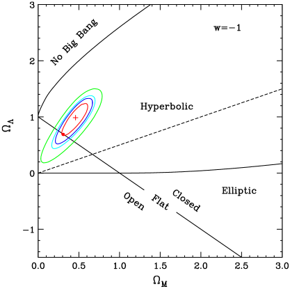
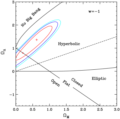
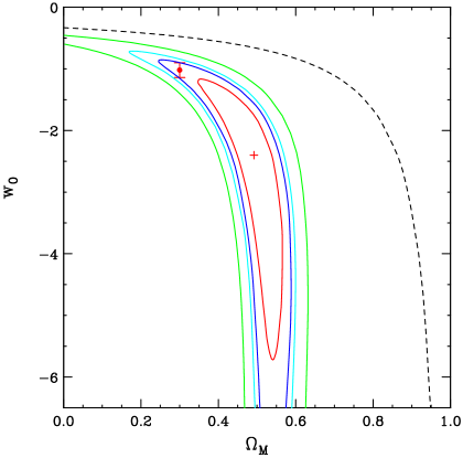
The gold data set gives joint confidence levels in the matter - dark energy plane with that are more restrictive than the earlier data and in good agreement with other constraints four . This is shown in Fig. 1. Thus, perhaps, it is not too early to ask whether this data
can distinguish between simple models for . To investigate this question we use a few models such as , and to calculate a luminosity distance. We then minimize the of the difference between the measured and calculated luminosity distances in an attempt to determine the constant parameters and . WMAP wmap and other experiments SDSS have accurately determined the matter density and curvature, defined as
| (3) | |||
| (4) |
to be close to and . is the density of matter today, is the Hubble constant today, and . Nevertheless, because we would like to know to what extent the supernova data agrees with these other experiments, we will sometimes include and/or in our set of parameters to be fit despite the fact that this exacerbates the degeneracy problem that arises because the luminosity distance depends only on the sum of the matter, curvature and dark energy contributions.
In an earlier paper DR , we explored the sensitivity of the data in Refs. hiz ; super to simple assumptions about the dark energy density. Recently, many other papers have appeared fits ; greek which use the data of Refs. four ; tre1 ; tre2 to analyze numerous models of the dark energy. A paper which is close in spirit to this work and which we had the advantage of reading before we started this work is Ref. greek . While we disagree with some of the results and conclusions, there is still much to like about this reference; many more models were studied and physical motivation is given for some of the models. We, on the other hand, have chosen to consider only the simplest cases to remain as model-independent as possible.
Our results are not encouraging. The errors in the fitted parameters are often more than , in some cases much more. We estimate the error in itself is more than . Still some consistencies can be seen and some patterns discerned. And while the data is not manifestly in agreement with other experiments (e.g., and ) it is not in disagreement. One (negative) result that seems very clear is that the absolute value of cannot be used, at this time (i. e., from this data set), to discriminate between models for .
II Calculation of the luminosity distance and
The luminosity distance is given by
| (5) |
where is the Hubble parameter
| (6) | |||||
| (7) |
and is given by the equation of state
| (8) |
In Eq. (5) is used for (), is used for (), and the unmodified square bracket is used for .
Many references give models where is not obviously related to an equation of state. However, from Eq. (8) we see that , , and, given an explicit expression for ,
| (9) |
where the prime denotes a derivative with respect to . This equation can also be used to express the effects of extra dimensions as an effective .
Below we use the dimensionless luminosity distance
| (10) |
and the quantity that is compared to the data is where is a constant offset between the data and the theoretical expression. The comparison is made by calculating where
| (11) |
The sum is over the events contained in the gold set four and are the experimental errors in .
, through the equation of state , Eq. (1), depends on some set of parameters, , and we minimize by varying these parameters. also depends on but to minimize with respect to is trivial,
| (12) |
where and are given by
| (13) | |||||
| (14) |
Sometimes we use Eq. (12) for , sometimes we include as one of the parameters to be fit, and we have checked that we get the same result.
The data indicates that the universe was decelerating in the past and it is of interest to know when that changed. The acceleration is given by
| (15) | |||||
| (16) |
and, given from Eq. (6), and values for the parameters, it is straightforward to find where .
III Results
We consider three simple, rather ad hoc, expressions for the equation of state modelI
| (17) | |||||
| (18) | |||||
| (19) |
where and are constants. These expressions allow us to evaluate
| Model | ||||||
|---|---|---|---|---|---|---|
| I. | ||||||
| II. | ||||||
| III. | ||||||
| IV. | 172.5 | 0 | ||||
| V. | ||||||
| VI. | 177.1 | 0 | 0.3 | 0.7 | ||
| VII. | ||||||
| VIII. | ||||||
| IX. | 0.3 | |||||
| X. | 0 | |||||
| XI. | 0 | 0.3 | ||||
| XII. | 0 |
the integral in Eq. (8) and avoid having an integral within an integral. We minimize with respect to , (if relevant), , (or ), or some subset of these; sometimes we hold fixed at zero or fixed at or fixed at or some combination of these conditions. If a parameter is allowed to vary we impose no prior conditions on the values it may assume except for and .
It is not straightforward to minimize because the minimum is very shallow and very broad. We use two independent numerical codes to cross check, one is a slight generalization of programs (MRQMIN) given in Numerical Recipes NR , the other is a code called STEPIT jpc which is available on the web.
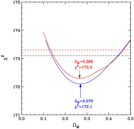
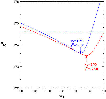
Our results are given in Table 1. The first 3 rows use Eq. (17), with either nothing, , or and fixed. The next 6 rows do the same for Eq. (18) and then for Eq. (19). The last 3 rows give some special cases. For each model we give the minimum value and the values of the parameters which give that value. The errors on the parameters are the confidence level uncertainties given for a particular parameter by finding the variation in that parameter which results in an increase of by when the other parameters are allowed to vary freely. Plots of how varies to the error in each parameter are shown in Fig. 2 for Models I (red curves)and VII (blue curves). If the
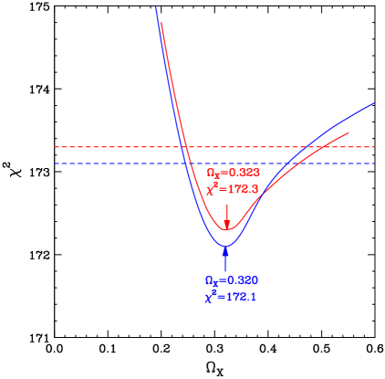
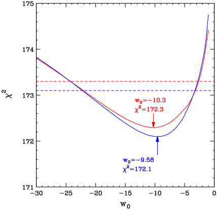
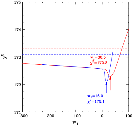
parameters in these models are restricted to the case of a flat cosmology, , the resulting errors of Models II and VIII are shown in Fig. 3.
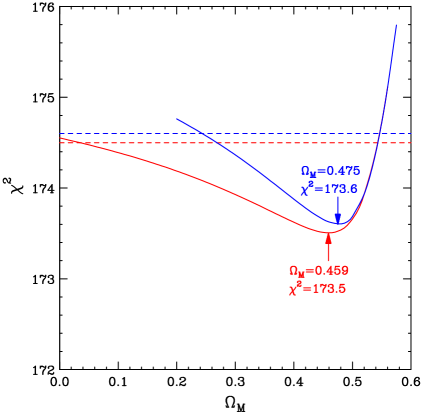
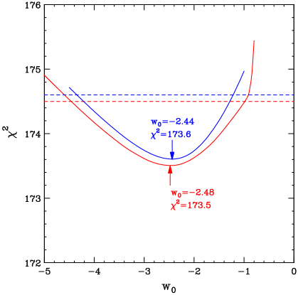
To try to get an estimate of the uncertainty in itself, and to check the stability of the numbers in Table 1, we have done approximately bootstrap simulations. These simulations consist of constructing new data sets by randomly selecting events from the original data set. We do enough such simulations that each event gets used about the same number of times. We then calculate the average for the simulations and, to find an error for , take the standard deviation of the set of . We also find the average and the standard deviation for each of the parameters. These results are given in Table 2. The values of the parameters and
| Model | |||||
|---|---|---|---|---|---|
| Ib. | |||||
| IIb. | |||||
| IIIb. | |||||
| IVb. | |||||
| Vb. | |||||
| VIb. | |||||
| VIIb. | |||||
| VIIIb. | |||||
| IXb. | |||||
| Xb. | |||||
| XIb. | |||||
| XIIb. |
the errors in the parameters are very consistent with those given in Table 1. In fact for the cases where only one or two parameters are fit they are almost identical. The values of for the individual simulations vary from to with a standard deviation of about 20. Thus, from these simulations, we conclude that the values in Table 1 are robust and that is uncertain by .
IV Conclusions
If we take the cosmological constant case (, ) and fit or we get the preferred answer of or (see Models X and XI in Table 1). Or if we hold and and fit we get the preferred answer of (Model VI). However, if we try to fit even two of the three as in Models V or XII, the fitted values are not the preferred ones although the errors are large enough to make the parameters consistent with the desired values. This can be seen in some detail in the confidence contours for Model V, shown in Fig. 4. Model XII, shown in more detail in Fig. 1, was our original
motivation.
Our Models III and IX are models 9 and 7 of Ref. greek . That paper used the 2003 data set tre1 ; tre2 ; when we ran with that data set, and included the extra error due to the peculiar velocity as in greek , we were able to find a smaller value for in both of these cases; perhaps we used a different expression for the pecular velocity error. In any case a smaller is not very important in view of the large uncertainty in indicated by the simulations. What is important, in view of this uncertainty, is that small relative values of do not indicate which models are a better fit. Also the ability to find the lowest is essential to determining the errors on the parameters; if the lowest is not found the errors will appear to be smaller than they actually are. We found much larger errors for the parameters than those given in Ref. greek and this seems not to be due to uncertainity in handling the pecular velocity error. For example our result for Model III is , .
If we include structure in , as in Models I, II, III, which use or VII, VIII, IX, which use , then the errors get very large and it is hard to draw any conclusions even if and are fixed. What does seem clear, from the similarity of the results for Models I and VII, II and VIII, and III and IX is that low events are still dominating. ( of Models VII, VIII, and IX should be compared with of Models I, II, and III.) The factor of in the denominator of Eq. (17) is effectively just . We have checked that this is also true for the gold plus silver data set. Thus comparing models for the equation of state of the dark energy will remain something of a mug’s game until there exists substantially more data at higher values of .
Acknowledgements.
We thank Rahul Malhotra, Megan Donahue, Mark Voit and Steve Zepf for useful discussions and Vinod Johri for a helpful communication. This research was supported in part by the National Science Foundation under Grant PHY-0244789 and by the United States Department of Energy under Contract No. DE-FG03-93ER40757.References
- (1) A. G. Riess et al., A. J. 116, 1009 (1998).
- (2) S. Perlmutter et al., Ap. J. 517, 565 (1999).
- (3) A. G. Riess et al., arXiv:astro-ph/0402512.
- (4) J. L. Tonry et al., Ap. J. 594, 1 (2003) [arXiv:astro-ph/0305008].
- (5) B. J. Barris et al., Ap. J. in press, arXiv:astro-ph/0310843.
- (6) C. L. Bennett et al., Ap. J. Suppl., Ser. 143, 1 (2003).
- (7) For a very nice small review see W. L. Freedman and M. S. Turner, Rev. Mod. Phys. 75, 1433 (2003).
- (8) D. A. Dicus and W. W. Repko, Phys. Rev. D 67, 083520 (2003).
- (9) E. V. Linder, arXiv:astro-ph/0406189; D. Parkinson, B. A. Bassett, E. J. Copeland, P. S. Corasaniti and M. Kunz, arXiv:astro-ph/0406018; R. A. Daly and S. G. Djorgovski, arXiv:astro-ph/0405550; Y. Gong, arXiv:astro-ph/0405446; Y. Wang, arXiv:astro-ph/0404484; H.K.Jassal, J.S.Bagla, T. Padmanabhan, arXiv:astro-ph/0404378; Y. G. Gong, X. M. Chen and C. K. Duan, arXiv:astro-ph/0404202; B. Feng, X. L. Wang and X. M. Zhang, arXiv:astro-ph/0404224; D. Huterer and A. Cooray, arXiv:astro-ph/0404062; U. Alam, V. Sahni and A. A. Starobinsky, arXiv:astro-ph/0403687; R. A. Daly and S. G. Djorgovski, arXiv:astro-ph/0403664; Y. Wang and M. Tegmark, arXiv:astro-ph/0403292; O. Bertolami, A. A. Sen, S. Sen and P. T. Silva, arXiv:astro-ph/0402387; Y. Wang and K. Freese, arXiv:astro-ph/0402208; Y. G. Gong and C. K. Duan, arXiv:astro-ph/0401530; D.F. Mota and C. van de Bruck, Astron. and Astrophys. 71, 421 (2004); Y. Wang and P. Mukherjee, Astrophys. J. 606, 654 (2004) [arXiv:astro-ph/0312192]; T. R. Choudhury and T. Padmanabhan, arXiv:astro-ph/0311622; U. Alam, V. Sahni, T. D. Saini and A. A. Starobinsky, arXiv:astro-ph/0311364; T. D. Saini, J. Weller and S. L. Bridle, Mon. Not. Roy. Astron. Soc. 348, 603 (2004) [arXiv:astro-ph/0305526]; T. R. Choudhury and T. Padmanabhan, Mon. Not. Roy. Astron. Soc. 344, 823 (2003) [arXiv:astro-ph/0212573].
- (10) S. Nesseris and L. Perivolaropoulos, astro-ph/0401556.
- (11) The first of these models, Eq. (17), appears in: M. Chevallier and D. Polarski, Int. J. Mod. Phys. D 10, 213 (2001) [arXiv:gr-qc/0009008]; see also: E. V. Linder, Phys. Rev. Lett. 90, 091301 (2003) [arXiv:astro-ph/0208512].
- (12) W. H. Press et al., Numerical Recipes, Cambridge University Press (1994), p. 526.
- (13) J. P. Chandler, Behavioral Science 14, 81 (1969).