The RR Lyrae Period-Luminosity Relation.
I. Theoretical Calibration

Abstract

We present a theoretical calibration of the RR Lyrae period-luminosity (PL) relation in the $UBVRIJHK$ Johnsons-Cousins-Glass system. Our theoretical work is based on calculations of synthetic horizontal branches (HBs) for several different metallicities, fully taking into account evolutionary effects besides the effect of chemical composition. Extensive tabulations of our results are provided, including convenient analytical formulae for the calculation of the coefficients of the period-luminosity relation in the different passbands as a function of HB type. We also provide “average” PL relations in $IJHK$, for applications in cases where the HB type is not known a priori; as well as a new calibration of the $M_{V}-{\rm[M/H]}$ relation. These can be summarized as follows:

$$M_{I}=0.471-1.132\,\log P+0.205\,\log Z,$$

$$M_{J}=-0.141-1.773\,\log P+0.190\,\log Z,$$

$$M_{H}=-0.551-2.313\,\log P+0.178\,\log Z,$$

$$M_{K}=-0.597-2.353\,\log P+0.175\,\log Z,$$

and

$$M_{V}=2.288+0.882\,\log Z+0.108\,(\log Z)^{2}.$$

1. Introduction

RR Lyrae (RRL) stars are the cornerstone of the Population II distance scale. Yet, unlike Cepheids, which have for almost a century been known to present a tight period-luminosity (PL) relation (Leavitt 1912), RRL have not been known for presenting a particularly noteworthy PL relation. Instead, most researchers have utilized an average relation between absolute visual magnitude and metallicity [Fe/H] when deriving RRL-based distances. This relation possesses several potential pitfalls, including a strong dependence on evolutionary effects (e.g., Demarque et al. 2000), a possible non-linearity as a function of [Fe/H] (e.g., Castellani, Chieffi, & Pulone 1991), and “pathological outliers” (e.g., Pritzl et al. 2002).

Figure 1.— Upper panels: Morphology of the HB in different bandpasses (left: $B$; middle: $V$; right: $I$). RRL variables are shown in gray, and non-variable stars in black. Lower panels: Corresponding RRL distributions in the absolute magnitude—log-period plane. The correlation coefficient $r$ is shown in the lower panels. All plots refer to an HB simulation with $Z=0.002$ and an intermediate HB type, as indicated in the upper panels.

To be sure, RRL have also been noted to follow a PL relation, but only in the $K$ band (Longmore, Fernley, & Jameson 1986). This is in sharp contrast with the case of the Cepheids, which follow tight PL relations both in the visual and in the near-infrared (see, e.g., Tanvir 1999). The reason why Cepheids present a tight PL relation irrespective of bandpass is that these stars cover a large range in luminosities but only a modest range in temperatures. Conversely, RRL stars are restricted to the horizontal branch (HB) phase of low-mass stars, and thus necessarily cover a much more modest range in luminosities—so much so that, in their case, the range in temperature of the instability strip is as important as, if not more important than, the range in luminosities of RRL stars, in determining their range in periods. Therefore, RRL stars may indeed present PL relations, but only if the bolometric corrections are such as to lead to a large range in absolute magnitudes when going from the blue to the red sides of the instability strip—as is indeed the case in $K$.

The purpose of the present paper, then, is to perform the first systematic analysis of whether a useful RRL PL relation may also be present in other bandpasses besides $K$. In particular, we expect that, using bandpasses in which the HB is not quite “horizontal” at the RRL level, a PL relation should indeed be present. Since the HB around the RRL region becomes distinctly non-horizontal both towards the near-ultraviolet (e.g., Fig. 4 in Ferraro et al. 1998) and towards the near-infrared (e.g., Davidge & Courteau 1999), we present a full analysis of the slope and zero point of the RRL PL relation in the Johnsons-Cousins-Glass system, from $U$ to $K$, including also $BVRIJH$.

2. Models

The HB simulations employed in the present paper are similar to those described in Catelan (2004a), to which the reader is referred for further details and references about the HB synthesis method. The evolutionary tracks employed here are those computed by Catelan et al. (1998) for $Z=0.001$ and $Z=0.0005$, and by Sweigart & Catelan (1998) for $Z=0.002$ and $Z=0.006$, and assume a main-sequence helium abundance of 23% by mass and scaled-solar compositions. The mass distribution is represented by a normal deviate with a mass dispersion $\sigma_{M}=0.020\,M_{\odot}$. For the purposes of the present paper, we have added to this code bolometric corrections from Girardi et al. (2002) for $URJHK$ over the relevant ranges of temperature and gravity. The width of the instability strip is taken as $\Delta\log T_{\rm eff}=0.075$, which provides the temperature of the red edge of the instability strip for each star once its blue edge has been computed on the basis of RRL pulsation theory results. More specifically, the instability strip blue edge adopted in this paper is based on equation (1) of Caputo et al. (1987), which provides a fit to Stellingwerf’s (1984) results—except that a shift by $-200$ K to the temperature values thus derived was applied in order to improve agreement with more recent theoretical prescriptions (see §6 in Catelan 2004a for a detailed discussion). We include both fundamental-mode (RRab) and “fundamentalized” first-overtone (RRc) variables in our final PL relations. The computed periods are based on equation (4) in Caputo, Marconi, & Santolamazza (1998), which represents an updated version of the van Albada & Baker (1971) period-mean density relation.

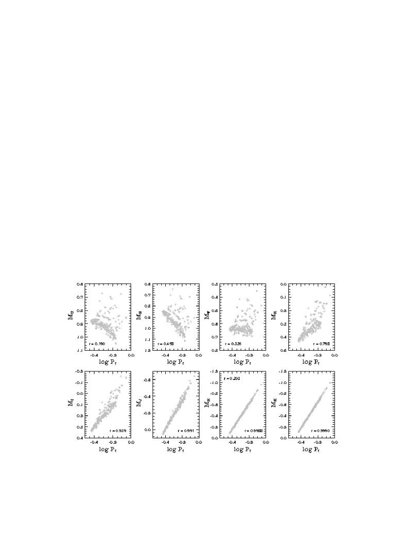
Figure 2.— PL relations in several different passbands. Upper panels: $U$ (left), $B$, $V$, $R$ (right). Lower panels: $I$ (left), $J$, $H$, $K$ (right). The correlation coefficient is shown in all panels. All plots refer to an HB simulation with $Z=0.001$ and an intermediate HB type.

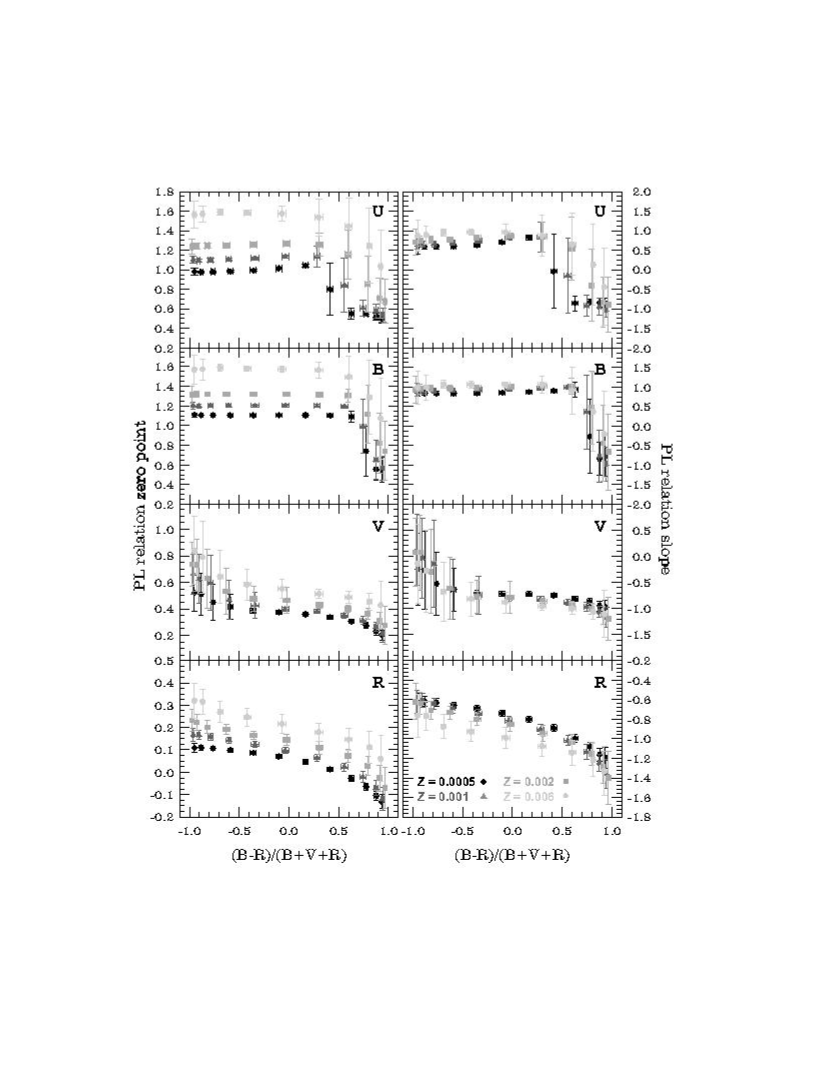
Figure 3.— Theoretically calibrated PL relations in the $UBVR$ passbands (from top to bottom), for the four indicated metallicities. The zero points (left panels) and slopes (right panels) are given as a function of the Lee-Zinn HB morphology indicator.

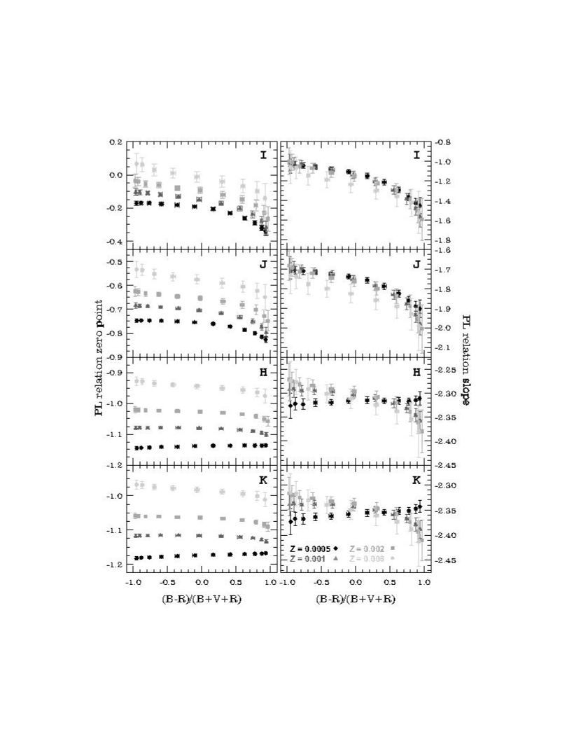
Figure 4.— As in Figure 3, but for $IJHK$ (from top to bottom).

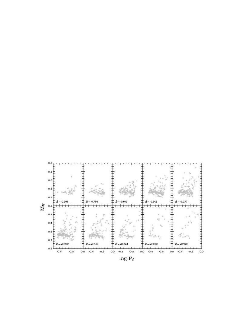
Figure 5.— Variation in the $M_{U}-\log P$ relation as a function of HB type, for a metallicity $Z=0.001$. The HB morphology, indicated by the $\mathscr{L}$ value, becomes bluer from upper left to lower right. For each HB type, only the first in the series of 100 simulations used to compute the average coefficients shown in Figures 3 and 4 and Table 1 was chosen to produce this figure.

Figure 6.— As in Figure 5, but for the $M_{B}-\log P$ relation.

Figure 7.— As in Figure 5, but for the $M_{V}-\log P$ relation.

Figure 8.— As in Figure 5, but for the $M_{R}-\log P$ relation.

Figure 9.— As in Figure 5, but for the $M_{I}-\log P$ relation.

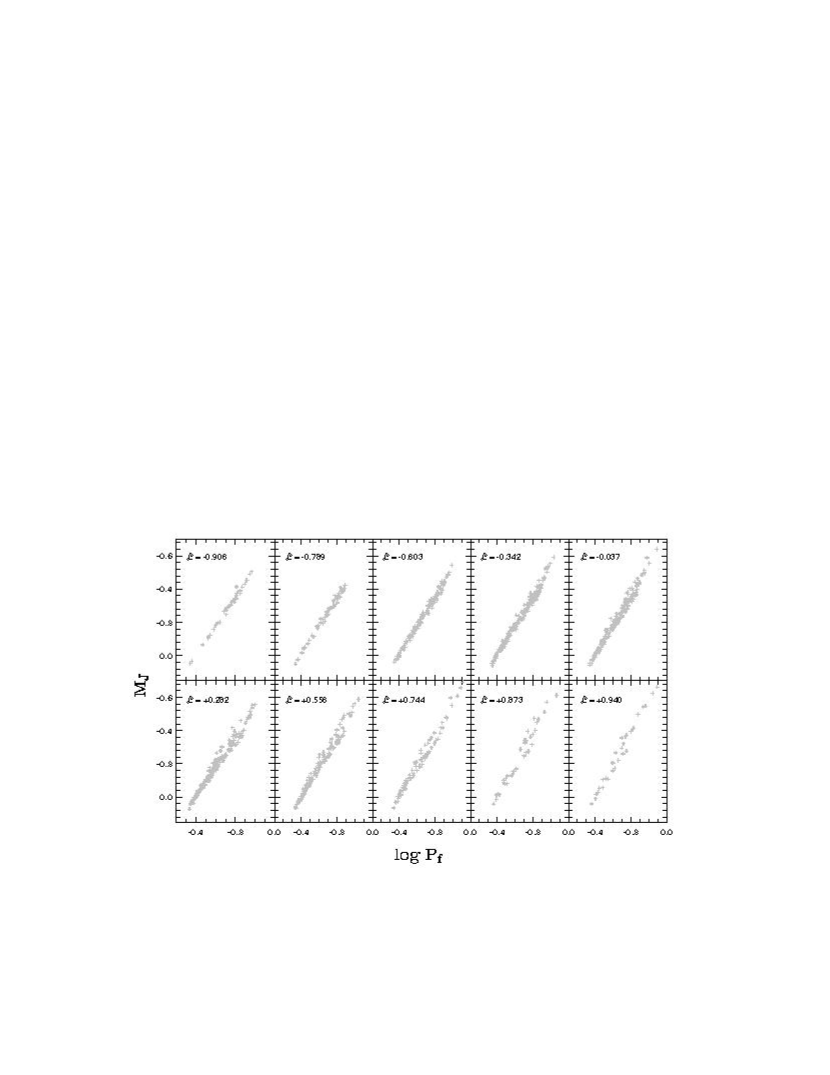
Figure 10.— As in Figure 5, but for the $M_{J}-\log P$ relation.

Figure 11.— As in Figure 5, but for the $M_{H}-\log P$ relation.

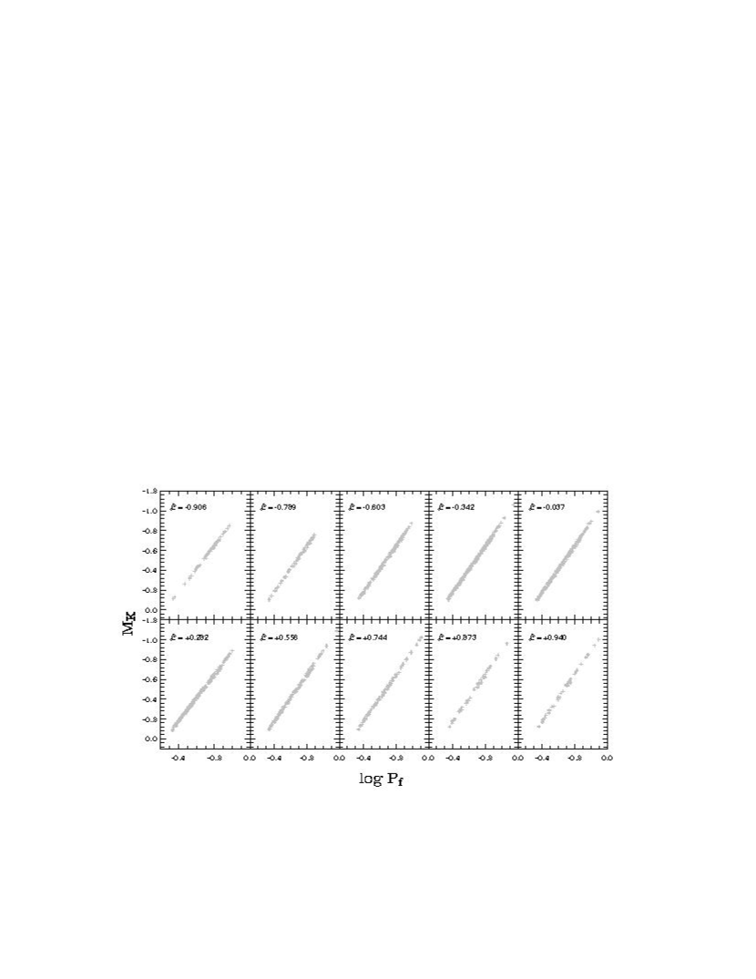
Figure 12.— As in Figure 5, but for the $M_{K}-\log P$ relation.

In order to study the dependence of the zero point and slope of the RRL PL relation with both HB type and metallicity, we have computed, for each metallicity, sequences of HB simulations which produce from very blue to very red HB types. These simulations are standard, and do not include such effects as HB bimodality or the impact of second parameters other than mass loss on the red giant branch (RGB) or age. For each such simulation, linear relations of the type $M_{X}=a+b\,\log P$, in which $X$ represents any of the $UBVRIJHK$ bandpasses, were obtained using the Isobe et al. (1990) “OLS bisector” technique. It is crucial that, if these relations are to be compared against empirical data to derive distances, precisely the same recipe be employed in the analysis of these data as well, particularly in cases in which the correlation coefficient is not very close to 1. The final result for each HB morphology actually represents the average $a$, $b$ values over 100 HB simulations with 500 stars each.

Table 1RRL PL Relation in $U$: Coefficients of the Fits

$\mathscr{L}$	$\sigma({\mathscr{L}})$	$a$	$\sigma(a)$	$b$	$\sigma(b)$
$Z=0.0005$
$0.934$	$0.013$	$0.497$	$0.042$	$-0.863$	$0.129$
$0.877$	$0.018$	$0.519$	$0.034$	$-0.849$	$0.110$
$0.776$	$0.022$	$0.547$	$0.024$	$-0.827$	$0.079$
$0.627$	$0.027$	$0.552$	$0.055$	$-0.860$	$0.192$
$0.414$	$0.028$	$0.799$	$0.267$	$-0.037$	$0.949$
$0.167$	$0.029$	$1.045$	$0.014$	$0.825$	$0.058$
$-0.102$	$0.031$	$1.013$	$0.010$	$0.706$	$0.048$
$-0.358$	$0.031$	$0.993$	$0.010$	$0.630$	$0.046$
$-0.590$	$0.025$	$0.983$	$0.009$	$0.595$	$0.041$
$-0.765$	$0.021$	$0.980$	$0.010$	$0.586$	$0.050$
$-0.883$	$0.014$	$0.977$	$0.013$	$0.587$	$0.068$
$-0.950$	$0.010$	$0.979$	$0.038$	$0.605$	$0.200$
$Z=0.0010$
$0.940$	$0.011$	$0.537$	$0.070$	$-1.027$	$0.191$
$0.873$	$0.018$	$0.580$	$0.070$	$-0.952$	$0.217$
$0.744$	$0.025$	$0.609$	$0.083$	$-0.923$	$0.275$
$0.556$	$0.034$	$0.844$	$0.277$	$-0.151$	$0.962$
$0.282$	$0.033$	$1.134$	$0.109$	$0.833$	$0.376$
$-0.037$	$0.035$	$1.136$	$0.012$	$0.818$	$0.055$
$-0.342$	$0.036$	$1.117$	$0.011$	$0.741$	$0.047$
$-0.603$	$0.025$	$1.107$	$0.012$	$0.698$	$0.055$
$-0.789$	$0.022$	$1.098$	$0.017$	$0.659$	$0.081$
$-0.906$	$0.015$	$1.094$	$0.017$	$0.646$	$0.078$
$-0.963$	$0.008$	$1.104$	$0.034$	$0.701$	$0.169$
$Z=0.0020$
$0.965$	$0.009$	$0.675$	$0.224$	$-0.890$	$0.696$
$0.910$	$0.015$	$0.708$	$0.207$	$-0.826$	$0.643$
$0.794$	$0.025$	$0.853$	$0.286$	$-0.405$	$0.920$
$0.594$	$0.029$	$1.155$	$0.250$	$0.541$	$0.816$
$0.307$	$0.036$	$1.255$	$0.117$	$0.847$	$0.383$
$-0.023$	$0.034$	$1.268$	$0.015$	$0.865$	$0.066$
$-0.356$	$0.035$	$1.258$	$0.017$	$0.820$	$0.069$
$-0.630$	$0.032$	$1.248$	$0.017$	$0.771$	$0.069$
$-0.822$	$0.021$	$1.247$	$0.021$	$0.768$	$0.089$
$-0.928$	$0.012$	$1.242$	$0.030$	$0.739$	$0.127$
$-0.974$	$0.008$	$1.236$	$0.077$	$0.709$	$0.326$
$Z=0.0060$
$0.922$	$0.015$	$1.032$	$0.369$	$-0.439$	$0.985$
$0.810$	$0.021$	$1.243$	$0.383$	$0.128$	$1.034$
$0.601$	$0.034$	$1.445$	$0.285$	$0.648$	$0.792$
$0.298$	$0.039$	$1.535$	$0.186$	$0.871$	$0.520$
$-0.070$	$0.039$	$1.574$	$0.077$	$0.959$	$0.210$
$-0.420$	$0.036$	$1.582$	$0.024$	$0.958$	$0.075$
$-0.693$	$0.025$	$1.586$	$0.032$	$0.954$	$0.095$
$-0.868$	$0.018$	$1.571$	$0.079$	$0.887$	$0.229$
$-0.951$	$0.012$	$1.564$	$0.136$	$0.866$	$0.398$

3. Genesis of the RRL PL Relation

In Figure 1, we show an HB simulation computed for a metallicity $Z=0.002$ and an intermediate HB morphology, indicated by a value of the Lee-Zinn type $\mathscr{L}\equiv(B-R)/(B+V+R)=-0.05$ (where $B$, $V$, and $R$ are the numbers of blue, variable, and red HB stars, respectively). Even using only the more usual $BVI$ bandpasses of the Johnson-Cousins system, the change in the detailed morphology of the HB with the passband adopted is obvious. In the middle upper panel, one can see the traditional display of a “horizontal” HB, as obtained in the $M_{V}$, $\bv$ plane. As a consequence, one can see, in the middle lower panel, that no PL relation results using this bandpass. On the other hand, the upper left panel shows the same simulation in the $M_{B}$, $\bv$ plane. One clearly sees now that the HB is not anymore “horizontal.” This has a clear impact upon the resulting PL relation (lower left panel): now one does see an indication of a correlation between period and $M_{B}$, though with a large scatter. The reason for this scatter is that the effects of luminosity and temperature variations upon the expected periods are almost orthogonal in this plane. Now one can also see, in the upper right panel, that the HB is also not quite horizontal in the $M_{I}$, $\bv$ plane—only that now, in comparison with the $M_{B}$, $\bv$ plane, the stars that look brighter are also the ones that are cooler. Since a decrease in temperature, as well as an increase in brightness, both lead to longer periods, one expects the effects of brightness and temperature upon the periods to be more nearly parallel when using $I$. This is indeed what happens, as can be seen in the bottom right panel. We now find a quite reasonable PL relation, with much less scatter than was the case in $B$.

Table 2RRL PL Relation in $B$: Coefficients of the Fits

$\mathscr{L}$	$\sigma({\mathscr{L}})$	$a$	$\sigma(a)$	$b$	$\sigma(b)$
$Z=0.0005$
$0.934$	$0.013$	$0.553$	$0.124$	$-0.763$	$0.524$
$0.877$	$0.018$	$0.555$	$0.110$	$-0.838$	$0.431$
$0.776$	$0.022$	$0.739$	$0.257$	$-0.263$	$0.940$
$0.627$	$0.027$	$1.093$	$0.058$	$0.933$	$0.199$
$0.414$	$0.028$	$1.104$	$0.013$	$0.899$	$0.044$
$0.167$	$0.029$	$1.107$	$0.012$	$0.873$	$0.040$
$-0.102$	$0.031$	$1.106$	$0.010$	$0.851$	$0.037$
$-0.358$	$0.031$	$1.105$	$0.010$	$0.836$	$0.035$
$-0.590$	$0.025$	$1.105$	$0.010$	$0.831$	$0.036$
$-0.765$	$0.021$	$1.107$	$0.011$	$0.839$	$0.047$
$-0.883$	$0.014$	$1.105$	$0.013$	$0.838$	$0.060$
$-0.950$	$0.010$	$1.108$	$0.020$	$0.853$	$0.100$
$Z=0.0010$
$0.940$	$0.011$	$0.568$	$0.123$	$-0.966$	$0.437$
$0.873$	$0.018$	$0.651$	$0.196$	$-0.768$	$0.665$
$0.744$	$0.025$	$0.994$	$0.271$	$0.362$	$0.944$
$0.556$	$0.034$	$1.195$	$0.016$	$1.001$	$0.048$
$0.282$	$0.033$	$1.202$	$0.013$	$0.973$	$0.046$
$-0.037$	$0.035$	$1.206$	$0.015$	$0.955$	$0.051$
$-0.342$	$0.036$	$1.205$	$0.013$	$0.935$	$0.044$
$-0.603$	$0.025$	$1.205$	$0.013$	$0.923$	$0.048$
$-0.789$	$0.022$	$1.203$	$0.015$	$0.906$	$0.067$
$-0.906$	$0.015$	$1.200$	$0.019$	$0.895$	$0.076$
$-0.963$	$0.008$	$1.207$	$0.036$	$0.930$	$0.164$
$Z=0.0020$
$0.965$	$0.009$	$0.741$	$0.300$	$-0.659$	$0.974$
$0.910$	$0.015$	$0.822$	$0.305$	$-0.442$	$0.972$
$0.794$	$0.025$	$1.116$	$0.294$	$0.466$	$0.939$
$0.594$	$0.029$	$1.302$	$0.068$	$1.022$	$0.214$
$0.307$	$0.036$	$1.315$	$0.017$	$1.024$	$0.059$
$-0.023$	$0.034$	$1.320$	$0.017$	$1.011$	$0.063$
$-0.356$	$0.035$	$1.319$	$0.018$	$0.990$	$0.066$
$-0.630$	$0.032$	$1.320$	$0.019$	$0.969$	$0.066$
$-0.822$	$0.021$	$1.320$	$0.021$	$0.969$	$0.080$
$-0.928$	$0.012$	$1.321$	$0.033$	$0.955$	$0.125$
$-0.974$	$0.008$	$1.315$	$0.084$	$0.923$	$0.346$
$Z=0.0060$
$0.922$	$0.015$	$1.072$	$0.413$	$-0.205$	$1.110$
$0.810$	$0.021$	$1.288$	$0.377$	$0.370$	$1.020$
$0.601$	$0.034$	$1.495$	$0.212$	$0.907$	$0.589$
$0.298$	$0.039$	$1.563$	$0.079$	$1.067$	$0.222$
$-0.070$	$0.039$	$1.574$	$0.027$	$1.068$	$0.069$
$-0.420$	$0.036$	$1.580$	$0.028$	$1.060$	$0.078$
$-0.693$	$0.025$	$1.588$	$0.035$	$1.065$	$0.099$
$-0.868$	$0.018$	$1.573$	$0.108$	$0.992$	$0.317$
$-0.951$	$0.012$	$1.571$	$0.145$	$0.987$	$0.420$

The same concepts explain the behavior of the RRL PL relation in the other passbands of the Johnson-Cousins-Glass system, which becomes tighter both towards the near-ultraviolet and towards the near-infrared, as compared to the visual. In Figure 2, we show the PL relations in all of the $UBVR$ (upper panels) and $IJHK$ (lower panels) bandpasses, for a synthetic HB with a morphology similar to that shown in Figure 1, but computed for a metallicity $Z=0.001$ (the results are qualitatively similar for all metallicities). As one can see, as one moves redward from $V$, where the HB is effectively horizontal at the RRL level, an increasingly tighter PL relation develops. Conversely, as one moves from $V$ towards the ultraviolet, the expectation is also for the PL relation to become increasingly tighter—which is confirmed by the plot for $B$. In the case of broadband $U$, as can be seen, the expected tendency is not fully confirmed, an effect which we attribute to the complicating impact of the Balmer jump upon the predicted bolometric corrections in the region of interest. An investigation of the RRL PL relation in Strömgren $u$ (e.g., Clem et al. 2004), which is much less affected by the Balmer discontinuity (and might accordingly produce a tighter PL relation than in broadband $U$), as well as of the UV domain, should thus prove of interest, but has not been attempted in the present work.

Table 3RRL PL Relation in $V$: Coefficients of the Fits

$\mathscr{L}$	$\sigma({\mathscr{L}})$	$a$	$\sigma(a)$	$b$	$\sigma(b)$
$Z=0.0005$
$0.934$	$0.013$	$0.203$	$0.038$	$-0.973$	$0.126$
$0.877$	$0.018$	$0.231$	$0.029$	$-0.947$	$0.096$
$0.776$	$0.022$	$0.274$	$0.021$	$-0.871$	$0.065$
$0.627$	$0.027$	$0.305$	$0.017$	$-0.815$	$0.049$
$0.414$	$0.028$	$0.338$	$0.013$	$-0.749$	$0.041$
$0.167$	$0.029$	$0.360$	$0.013$	$-0.723$	$0.045$
$-0.102$	$0.031$	$0.374$	$0.014$	$-0.714$	$0.053$
$-0.358$	$0.031$	$0.385$	$0.017$	$-0.723$	$0.069$
$-0.590$	$0.025$	$0.415$	$0.096$	$-0.639$	$0.409$
$-0.765$	$0.021$	$0.448$	$0.134$	$-0.530$	$0.600$
$-0.883$	$0.014$	$0.510$	$0.158$	$-0.271$	$0.745$
$-0.950$	$0.010$	$0.520$	$0.137$	$-0.249$	$0.689$
$Z=0.0010$
$0.940$	$0.011$	$0.215$	$0.065$	$-1.162$	$0.188$
$0.873$	$0.018$	$0.265$	$0.036$	$-1.060$	$0.103$
$0.744$	$0.025$	$0.312$	$0.028$	$-0.967$	$0.088$
$0.556$	$0.034$	$0.351$	$0.019$	$-0.879$	$0.057$
$0.282$	$0.033$	$0.383$	$0.016$	$-0.815$	$0.044$
$-0.037$	$0.035$	$0.399$	$0.016$	$-0.801$	$0.057$
$-0.342$	$0.036$	$0.428$	$0.096$	$-0.741$	$0.359$
$-0.603$	$0.025$	$0.468$	$0.147$	$-0.627$	$0.567$
$-0.789$	$0.022$	$0.596$	$0.205$	$-0.146$	$0.824$
$-0.906$	$0.015$	$0.625$	$0.183$	$-0.037$	$0.762$
$-0.963$	$0.008$	$0.664$	$0.152$	$0.126$	$0.678$
$Z=0.0020$
$0.965$	$0.009$	$0.276$	$0.142$	$-1.195$	$0.415$
$0.910$	$0.015$	$0.310$	$0.063$	$-1.118$	$0.172$
$0.794$	$0.025$	$0.361$	$0.041$	$-1.007$	$0.107$
$0.594$	$0.029$	$0.401$	$0.024$	$-0.919$	$0.068$
$0.307$	$0.036$	$0.429$	$0.023$	$-0.865$	$0.061$
$-0.023$	$0.034$	$0.464$	$0.097$	$-0.784$	$0.314$
$-0.356$	$0.035$	$0.477$	$0.092$	$-0.771$	$0.312$
$-0.630$	$0.032$	$0.533$	$0.171$	$-0.610$	$0.590$
$-0.822$	$0.021$	$0.630$	$0.224$	$-0.293$	$0.796$
$-0.928$	$0.012$	$0.733$	$0.196$	$0.072$	$0.715$
$-0.974$	$0.008$	$0.737$	$0.170$	$0.073$	$0.654$
$Z=0.0060$
$0.922$	$0.015$	$0.428$	$0.177$	$-1.103$	$0.445$
$0.810$	$0.021$	$0.454$	$0.065$	$-1.061$	$0.152$
$0.601$	$0.034$	$0.487$	$0.046$	$-1.001$	$0.113$
$0.298$	$0.039$	$0.513$	$0.033$	$-0.957$	$0.084$
$-0.070$	$0.039$	$0.551$	$0.074$	$-0.880$	$0.201$
$-0.420$	$0.036$	$0.584$	$0.117$	$-0.815$	$0.325$
$-0.693$	$0.025$	$0.642$	$0.201$	$-0.677$	$0.561$
$-0.868$	$0.018$	$0.789$	$0.273$	$-0.280$	$0.781$
$-0.951$	$0.012$	$0.840$	$0.257$	$-0.142$	$0.748$

4. The RRL PL Relation Calibrated

In Figure 3, we show the slope (left panels) and zero point (right panels) of the theoretically-calibrated RRL PL relation, in $UBVR$ (from top to bottom) and for four different metallicities (as indicated by different symbols and shades of gray; see the lower right panel). Each datapoint corresponds to the average over 100 simulations with 500 stars in each. The “error bars” correspond to the standard deviation of the mean over these 100 simulations. Figure 4 is analogous to Figure 3, but shows instead our results for the $IJHK$ passbands (from top to bottom). It should be noted that, for all bandpasses, the coefficients of the PL relations are much more subject to statistical fluctuations at the extremes in HB type (both very red and very blue), due to the smaller numbers of RRL variables for these HB types. In terms of Figures 3 and 4, this is indicated by an increase in the size of the “error bars” at both the blue and red ends of the relations.

Table 4RRL PL Relation in $R$: Coefficients of the Fits

$\mathscr{L}$	$\sigma({\mathscr{L}})$	$a$	$\sigma(a)$	$b$	$\sigma(b)$
$Z=0.0005$
$0.934$	$0.013$	$-0.132$	$0.031$	$-1.195$	$0.108$
$0.877$	$0.018$	$-0.106$	$0.021$	$-1.163$	$0.068$
$0.776$	$0.022$	$-0.065$	$0.017$	$-1.081$	$0.049$
$0.627$	$0.027$	$-0.028$	$0.014$	$-0.996$	$0.040$
$0.414$	$0.028$	$0.013$	$0.011$	$-0.891$	$0.033$
$0.167$	$0.029$	$0.047$	$0.011$	$-0.801$	$0.033$
$-0.102$	$0.031$	$0.070$	$0.009$	$-0.738$	$0.031$
$-0.358$	$0.031$	$0.087$	$0.008$	$-0.689$	$0.029$
$-0.590$	$0.025$	$0.098$	$0.008$	$-0.656$	$0.032$
$-0.765$	$0.021$	$0.107$	$0.010$	$-0.630$	$0.039$
$-0.883$	$0.014$	$0.110$	$0.012$	$-0.619$	$0.055$
$-0.950$	$0.010$	$0.110$	$0.020$	$-0.634$	$0.102$
$Z=0.0010$
$0.940$	$0.011$	$-0.119$	$0.051$	$-1.354$	$0.148$
$0.873$	$0.018$	$-0.070$	$0.032$	$-1.248$	$0.089$
$0.744$	$0.025$	$-0.021$	$0.026$	$-1.134$	$0.078$
$0.556$	$0.034$	$0.023$	$0.018$	$-1.017$	$0.054$
$0.282$	$0.033$	$0.065$	$0.017$	$-0.906$	$0.051$
$-0.037$	$0.035$	$0.098$	$0.015$	$-0.815$	$0.047$
$-0.342$	$0.036$	$0.125$	$0.014$	$-0.740$	$0.045$
$-0.603$	$0.025$	$0.143$	$0.014$	$-0.687$	$0.049$
$-0.789$	$0.022$	$0.159$	$0.016$	$-0.639$	$0.058$
$-0.906$	$0.015$	$0.167$	$0.019$	$-0.610$	$0.070$
$-0.963$	$0.008$	$0.167$	$0.027$	$-0.623$	$0.116$
$Z=0.0020$
$0.965$	$0.009$	$-0.071$	$0.092$	$-1.401$	$0.268$
$0.910$	$0.015$	$-0.027$	$0.059$	$-1.290$	$0.163$
$0.794$	$0.025$	$0.027$	$0.043$	$-1.158$	$0.118$
$0.594$	$0.029$	$0.074$	$0.028$	$-1.039$	$0.082$
$0.307$	$0.036$	$0.110$	$0.029$	$-0.948$	$0.082$
$-0.023$	$0.034$	$0.145$	$0.024$	$-0.854$	$0.070$
$-0.356$	$0.035$	$0.165$	$0.020$	$-0.803$	$0.061$
$-0.630$	$0.032$	$0.191$	$0.022$	$-0.732$	$0.067$
$-0.822$	$0.021$	$0.201$	$0.029$	$-0.708$	$0.095$
$-0.928$	$0.012$	$0.224$	$0.036$	$-0.640$	$0.116$
$-0.974$	$0.008$	$0.233$	$0.049$	$-0.619$	$0.183$
$Z=0.0060$
$0.922$	$0.015$	$0.060$	$0.103$	$-1.332$	$0.252$
$0.810$	$0.021$	$0.111$	$0.070$	$-1.217$	$0.168$
$0.601$	$0.034$	$0.147$	$0.051$	$-1.142$	$0.127$
$0.298$	$0.039$	$0.179$	$0.041$	$-1.076$	$0.106$
$-0.070$	$0.039$	$0.217$	$0.041$	$-0.991$	$0.103$
$-0.420$	$0.036$	$0.246$	$0.039$	$-0.928$	$0.101$
$-0.693$	$0.025$	$0.270$	$0.048$	$-0.876$	$0.125$
$-0.868$	$0.018$	$0.315$	$0.055$	$-0.767$	$0.146$
$-0.951$	$0.012$	$0.320$	$0.080$	$-0.763$	$0.221$

The slopes and zero points for the $UBVRIJHK$ calibrations are given in Tables 1 through 8, respectively. Appropriate values for any given HB morphology may be obtained from these tables by direct interpolation, or by using suitable interpolation formulae (Catelan 2004b), which we now proceed to describe in more detail.

Table 5RRL PL Relation in $I$: Coefficients of the Fits

$\mathscr{L}$	$\sigma({\mathscr{L}})$	$a$	$\sigma(a)$	$b$	$\sigma(b)$
$Z=0.0005$
$0.934$	$0.013$	$-0.343$	$0.023$	$-1.453$	$0.082$
$0.877$	$0.018$	$-0.322$	$0.015$	$-1.426$	$0.046$
$0.776$	$0.022$	$-0.291$	$0.012$	$-1.364$	$0.036$
$0.627$	$0.027$	$-0.261$	$0.010$	$-1.294$	$0.030$
$0.414$	$0.028$	$-0.231$	$0.009$	$-1.215$	$0.027$
$0.167$	$0.029$	$-0.207$	$0.008$	$-1.150$	$0.026$
$-0.102$	$0.031$	$-0.192$	$0.007$	$-1.109$	$0.022$
$-0.358$	$0.031$	$-0.182$	$0.006$	$-1.080$	$0.020$
$-0.590$	$0.025$	$-0.176$	$0.006$	$-1.060$	$0.023$
$-0.765$	$0.021$	$-0.171$	$0.007$	$-1.044$	$0.029$
$-0.883$	$0.014$	$-0.170$	$0.008$	$-1.038$	$0.037$
$-0.950$	$0.010$	$-0.171$	$0.014$	$-1.050$	$0.070$
$Z=0.0010$
$0.940$	$0.011$	$-0.318$	$0.037$	$-1.568$	$0.107$
$0.873$	$0.018$	$-0.279$	$0.025$	$-1.482$	$0.068$
$0.744$	$0.025$	$-0.239$	$0.019$	$-1.385$	$0.057$
$0.556$	$0.034$	$-0.204$	$0.014$	$-1.292$	$0.042$
$0.282$	$0.033$	$-0.172$	$0.013$	$-1.208$	$0.039$
$-0.037$	$0.035$	$-0.148$	$0.012$	$-1.140$	$0.037$
$-0.342$	$0.036$	$-0.130$	$0.011$	$-1.089$	$0.034$
$-0.603$	$0.025$	$-0.119$	$0.010$	$-1.055$	$0.033$
$-0.789$	$0.022$	$-0.110$	$0.011$	$-1.028$	$0.037$
$-0.906$	$0.015$	$-0.106$	$0.014$	$-1.012$	$0.051$
$-0.963$	$0.008$	$-0.105$	$0.020$	$-1.013$	$0.086$
$Z=0.0020$
$0.965$	$0.009$	$-0.265$	$0.074$	$-1.592$	$0.216$
$0.910$	$0.015$	$-0.230$	$0.047$	$-1.503$	$0.128$
$0.794$	$0.025$	$-0.185$	$0.035$	$-1.390$	$0.097$
$0.594$	$0.029$	$-0.148$	$0.023$	$-1.295$	$0.067$
$0.307$	$0.036$	$-0.120$	$0.022$	$-1.225$	$0.062$
$-0.023$	$0.034$	$-0.094$	$0.018$	$-1.154$	$0.052$
$-0.356$	$0.035$	$-0.080$	$0.014$	$-1.119$	$0.044$
$-0.630$	$0.032$	$-0.062$	$0.016$	$-1.070$	$0.048$
$-0.822$	$0.021$	$-0.056$	$0.020$	$-1.054$	$0.066$
$-0.928$	$0.012$	$-0.041$	$0.025$	$-1.011$	$0.080$
$-0.974$	$0.008$	$-0.036$	$0.037$	$-0.999$	$0.137$
$Z=0.0060$
$0.922$	$0.015$	$-0.142$	$0.088$	$-1.523$	$0.214$
$0.810$	$0.021$	$-0.098$	$0.057$	$-1.423$	$0.139$
$0.601$	$0.034$	$-0.068$	$0.042$	$-1.358$	$0.104$
$0.298$	$0.039$	$-0.042$	$0.034$	$-1.302$	$0.086$
$-0.070$	$0.039$	$-0.013$	$0.033$	$-1.237$	$0.083$
$-0.420$	$0.036$	$0.010$	$0.031$	$-1.188$	$0.080$
$-0.693$	$0.025$	$0.030$	$0.037$	$-1.145$	$0.098$
$-0.868$	$0.018$	$0.062$	$0.042$	$-1.068$	$0.112$
$-0.951$	$0.012$	$0.066$	$0.061$	$-1.061$	$0.168$

4.1. Analytical Fits

As the plots in Figures 3 and 4 show, all bands show some dependence on both metallicity and HB type, though some of the effects clearly become less pronounced as one goes towards the near-infrared. Analysis of the data for each metallicity shows that, except for the $U$ and $B$ cases, the coefficients of all PL relations (at a fixed metallicity) can be well described by third-order polynomials, as follows:

Table 6RRL PL Relation in $J$: Coefficients of the Fits

$\mathscr{L}$	$\sigma({\mathscr{L}})$	$a$	$\sigma(a)$	$b$	$\sigma(b)$
$Z=0.0005$
$0.934$	$0.013$	$-0.826$	$0.012$	$-1.902$	$0.045$
$0.877$	$0.018$	$-0.815$	$0.007$	$-1.890$	$0.024$
$0.776$	$0.022$	$-0.800$	$0.007$	$-1.861$	$0.020$
$0.627$	$0.027$	$-0.786$	$0.006$	$-1.825$	$0.017$
$0.414$	$0.028$	$-0.772$	$0.005$	$-1.788$	$0.015$
$0.167$	$0.029$	$-0.760$	$0.005$	$-1.757$	$0.015$
$-0.102$	$0.031$	$-0.754$	$0.004$	$-1.739$	$0.012$
$-0.358$	$0.031$	$-0.750$	$0.003$	$-1.727$	$0.011$
$-0.590$	$0.025$	$-0.748$	$0.004$	$-1.717$	$0.014$
$-0.765$	$0.021$	$-0.747$	$0.004$	$-1.710$	$0.018$
$-0.883$	$0.014$	$-0.746$	$0.005$	$-1.706$	$0.021$
$-0.950$	$0.010$	$-0.747$	$0.008$	$-1.709$	$0.040$
$Z=0.0010$
$0.940$	$0.011$	$-0.795$	$0.020$	$-1.981$	$0.057$
$0.873$	$0.018$	$-0.774$	$0.014$	$-1.934$	$0.039$
$0.744$	$0.025$	$-0.751$	$0.010$	$-1.879$	$0.030$
$0.556$	$0.034$	$-0.733$	$0.008$	$-1.830$	$0.024$
$0.282$	$0.033$	$-0.717$	$0.007$	$-1.786$	$0.021$
$-0.037$	$0.035$	$-0.705$	$0.007$	$-1.752$	$0.020$
$-0.342$	$0.036$	$-0.696$	$0.006$	$-1.726$	$0.019$
$-0.603$	$0.025$	$-0.691$	$0.005$	$-1.710$	$0.017$
$-0.789$	$0.022$	$-0.687$	$0.006$	$-1.698$	$0.020$
$-0.906$	$0.015$	$-0.685$	$0.008$	$-1.689$	$0.030$
$-0.963$	$0.008$	$-0.684$	$0.011$	$-1.685$	$0.049$
$Z=0.0020$
$0.965$	$0.009$	$-0.748$	$0.042$	$-2.005$	$0.123$
$0.910$	$0.015$	$-0.728$	$0.027$	$-1.955$	$0.072$
$0.794$	$0.025$	$-0.702$	$0.020$	$-1.890$	$0.056$
$0.594$	$0.029$	$-0.681$	$0.013$	$-1.837$	$0.038$
$0.307$	$0.036$	$-0.667$	$0.012$	$-1.800$	$0.034$
$-0.023$	$0.034$	$-0.653$	$0.010$	$-1.763$	$0.028$
$-0.356$	$0.035$	$-0.647$	$0.008$	$-1.745$	$0.024$
$-0.630$	$0.032$	$-0.638$	$0.009$	$-1.721$	$0.027$
$-0.822$	$0.021$	$-0.635$	$0.011$	$-1.713$	$0.034$
$-0.928$	$0.012$	$-0.628$	$0.014$	$-1.691$	$0.044$
$-0.974$	$0.008$	$-0.625$	$0.020$	$-1.682$	$0.076$
$Z=0.0060$
$0.922$	$0.015$	$-0.649$	$0.052$	$-1.989$	$0.125$
$0.810$	$0.021$	$-0.623$	$0.033$	$-1.929$	$0.080$
$0.601$	$0.034$	$-0.606$	$0.024$	$-1.891$	$0.059$
$0.298$	$0.039$	$-0.591$	$0.019$	$-1.860$	$0.049$
$-0.070$	$0.039$	$-0.575$	$0.019$	$-1.826$	$0.047$
$-0.420$	$0.036$	$-0.563$	$0.017$	$-1.800$	$0.044$
$-0.693$	$0.025$	$-0.553$	$0.021$	$-1.777$	$0.053$
$-0.868$	$0.018$	$-0.536$	$0.023$	$-1.739$	$0.062$
$-0.951$	$0.012$	$-0.534$	$0.033$	$-1.733$	$0.092$

$$M_{X}=a+b\,\log P,$$ (1)

Table 7RRL PL Relation in $H$: Coefficients of the Fits

$\mathscr{L}$	$\sigma({\mathscr{L}})$	$a$	$\sigma(a)$	$b$	$\sigma(b)$
$Z=0.0005$
$0.934$	$0.013$	$-1.136$	$0.003$	$-2.311$	$0.013$
$0.877$	$0.018$	$-1.137$	$0.002$	$-2.315$	$0.009$
$0.776$	$0.022$	$-1.137$	$0.002$	$-2.317$	$0.008$
$0.627$	$0.027$	$-1.137$	$0.002$	$-2.316$	$0.007$
$0.414$	$0.028$	$-1.137$	$0.002$	$-2.316$	$0.006$
$0.167$	$0.029$	$-1.138$	$0.002$	$-2.315$	$0.007$
$-0.102$	$0.031$	$-1.139$	$0.002$	$-2.316$	$0.006$
$-0.358$	$0.031$	$-1.141$	$0.002$	$-2.320$	$0.006$
$-0.590$	$0.025$	$-1.142$	$0.002$	$-2.320$	$0.008$
$-0.765$	$0.021$	$-1.143$	$0.003$	$-2.323$	$0.011$
$-0.883$	$0.014$	$-1.144$	$0.003$	$-2.322$	$0.013$
$-0.950$	$0.010$	$-1.146$	$0.005$	$-2.327$	$0.027$
$Z=0.0010$
$0.940$	$0.011$	$-1.101$	$0.006$	$-2.358$	$0.019$
$0.873$	$0.018$	$-1.096$	$0.005$	$-2.346$	$0.014$
$0.744$	$0.025$	$-1.090$	$0.003$	$-2.332$	$0.009$
$0.556$	$0.034$	$-1.086$	$0.003$	$-2.322$	$0.009$
$0.282$	$0.033$	$-1.083$	$0.002$	$-2.310$	$0.007$
$-0.037$	$0.035$	$-1.081$	$0.002$	$-2.304$	$0.008$
$-0.342$	$0.036$	$-1.079$	$0.003$	$-2.297$	$0.008$
$-0.603$	$0.025$	$-1.079$	$0.002$	$-2.295$	$0.008$
$-0.789$	$0.022$	$-1.079$	$0.003$	$-2.295$	$0.011$
$-0.906$	$0.015$	$-1.080$	$0.004$	$-2.292$	$0.016$
$-0.963$	$0.008$	$-1.080$	$0.006$	$-2.292$	$0.025$
$Z=0.0020$
$0.965$	$0.009$	$-1.058$	$0.015$	$-2.380$	$0.045$
$0.910$	$0.015$	$-1.051$	$0.009$	$-2.361$	$0.025$
$0.794$	$0.025$	$-1.042$	$0.007$	$-2.339$	$0.021$
$0.594$	$0.029$	$-1.035$	$0.005$	$-2.321$	$0.014$
$0.307$	$0.036$	$-1.031$	$0.005$	$-2.308$	$0.013$
$-0.023$	$0.034$	$-1.027$	$0.004$	$-2.297$	$0.012$
$-0.356$	$0.035$	$-1.025$	$0.003$	$-2.291$	$0.010$
$-0.630$	$0.032$	$-1.023$	$0.004$	$-2.284$	$0.012$
$-0.822$	$0.021$	$-1.023$	$0.004$	$-2.282$	$0.014$
$-0.928$	$0.012$	$-1.021$	$0.006$	$-2.275$	$0.019$
$-0.974$	$0.008$	$-1.020$	$0.009$	$-2.271$	$0.034$
$Z=0.0060$
$0.922$	$0.015$	$-0.975$	$0.022$	$-2.381$	$0.053$
$0.810$	$0.021$	$-0.964$	$0.014$	$-2.355$	$0.035$
$0.601$	$0.034$	$-0.957$	$0.010$	$-2.338$	$0.026$
$0.298$	$0.039$	$-0.950$	$0.008$	$-2.325$	$0.021$
$-0.070$	$0.039$	$-0.944$	$0.008$	$-2.312$	$0.020$
$-0.420$	$0.036$	$-0.939$	$0.007$	$-2.301$	$0.019$
$-0.693$	$0.025$	$-0.935$	$0.009$	$-2.292$	$0.023$
$-0.868$	$0.018$	$-0.929$	$0.010$	$-2.277$	$0.027$
$-0.951$	$0.012$	$-0.928$	$0.014$	$-2.274$	$0.040$

with

$$a=\sum_{i=0}^{3}a_{i}\left(\mathscr{L}\right)^{i},\,\,\,\,b=\sum_{i=0}^{3}b_{i}\left(\mathscr{L}\right)^{i}.$$ (2)

For all of the $VRIJHK$ passbands, the $a_{i}$, $b_{i}$ coefficients are provided in Table 9.

Table 8RRL PL Relation in $K$: Coefficients of the Fits

$\mathscr{L}$	$\sigma({\mathscr{L}})$	$a$	$\sigma(a)$	$b$	$\sigma(b)$
$Z=0.0005$
$0.934$	$0.013$	$-1.168$	$0.002$	$-2.343$	$0.012$
$0.877$	$0.018$	$-1.169$	$0.002$	$-2.348$	$0.009$
$0.776$	$0.022$	$-1.170$	$0.002$	$-2.352$	$0.007$
$0.627$	$0.027$	$-1.171$	$0.002$	$-2.352$	$0.007$
$0.414$	$0.028$	$-1.172$	$0.002$	$-2.355$	$0.006$
$0.167$	$0.029$	$-1.173$	$0.002$	$-2.355$	$0.007$
$-0.102$	$0.031$	$-1.175$	$0.002$	$-2.358$	$0.006$
$-0.358$	$0.031$	$-1.177$	$0.002$	$-2.362$	$0.006$
$-0.590$	$0.025$	$-1.178$	$0.002$	$-2.364$	$0.008$
$-0.765$	$0.021$	$-1.180$	$0.003$	$-2.368$	$0.011$
$-0.883$	$0.014$	$-1.181$	$0.003$	$-2.367$	$0.013$
$-0.950$	$0.010$	$-1.183$	$0.005$	$-2.373$	$0.026$
$Z=0.0010$
$0.940$	$0.011$	$-1.133$	$0.005$	$-2.388$	$0.017$
$0.873$	$0.018$	$-1.128$	$0.004$	$-2.379$	$0.013$
$0.744$	$0.025$	$-1.124$	$0.003$	$-2.367$	$0.009$
$0.556$	$0.034$	$-1.121$	$0.003$	$-2.359$	$0.009$
$0.282$	$0.033$	$-1.118$	$0.002$	$-2.350$	$0.007$
$-0.037$	$0.035$	$-1.11$	$70.002$	$-2.345$	$0.008$
$-0.342$	$0.036$	$-1.11$	$50.002$	$-2.339$	$0.008$
$-0.603$	$0.025$	$-1.11$	$60.002$	$-2.338$	$0.008$
$-0.789$	$0.022$	$-1.11$	$70.003$	$-2.339$	$0.011$
$-0.906$	$0.015$	$-1.11$	$70.004$	$-2.337$	$0.016$
$-0.963$	$0.008$	$-1.11$	$70.006$	$-2.338$	$0.024$
$Z=0.0020$
$0.965$	$0.009$	$-1.091$	$0.014$	$-2.410$	$0.041$
$0.910$	$0.015$	$-1.084$	$0.008$	$-2.393$	$0.022$
$0.794$	$0.025$	$-1.077$	$0.007$	$-2.374$	$0.019$
$0.594$	$0.029$	$-1.071$	$0.004$	$-2.358$	$0.013$
$0.307$	$0.036$	$-1.067$	$0.004$	$-2.347$	$0.012$
$-0.023$	$0.034$	$-1.064$	$0.004$	$-2.337$	$0.011$
$-0.356$	$0.035$	$-1.063$	$0.003$	$-2.333$	$0.010$
$-0.630$	$0.032$	$-1.061$	$0.004$	$-2.327$	$0.012$
$-0.822$	$0.021$	$-1.061$	$0.004$	$-2.325$	$0.013$
$-0.928$	$0.012$	$-1.059$	$0.006$	$-2.320$	$0.018$
$-0.974$	$0.008$	$-1.059$	$0.009$	$-2.317$	$0.032$
$Z=0.0060$
$0.922$	$0.015$	$-1.011$	$0.021$	$-2.413$	$0.049$
$0.810$	$0.021$	$-1.001$	$0.013$	$-2.389$	$0.032$
$0.601$	$0.034$	$-0.994$	$0.010$	$-2.374$	$0.024$
$0.298$	$0.039$	$-0.988$	$0.008$	$-2.362$	$0.019$
$-0.070$	$0.039$	$-0.983$	$0.008$	$-2.349$	$0.019$
$-0.420$	$0.036$	$-0.978$	$0.007$	$-2.340$	$0.018$
$-0.693$	$0.025$	$-0.974$	$0.008$	$-2.331$	$0.021$
$-0.868$	$0.018$	$-0.968$	$0.009$	$-2.317$	$0.025$
$-0.951$	$0.012$	$-0.968$	$0.013$	$-2.315$	$0.037$

5. Remarks on the RRL PL Relations

Figures 3 and 4 reveal a complex pattern for the variation of the coefficients of the PL relation as a function of HB morphology. While, as anticipated, the dependence on HB type (particularly the slope) is quite small for the redder passbands (note the much smaller axis scale range for the corresponding $H$ and $K$ plots than for the remaining ones), the same cannot be said with respect to the bluer passbands, particularly $U$ and $B$, for which one does see marked variations as one moves from very red to very blue HB types. This is obviously due to the much more important effects of evolution away from the zero-age HB in the bluer passbands. In order to fully highlight the changes in the PL relations in each of the considered bandpasses, we show, in Figures 5 through 12, the changes in the absolute magnitude–log-period distributions for each bandpass, from $U$ (Fig. 5) to $K$ (Fig. 12), for a representative metallicity, $Z=0.001$. Each figure is comprised of a mosaic of 10 plots, each for a different HB type, from very red (upper left panels) to very blue (lower right panels). In the bluer passbands, one can see the stars that are evolved away from a position on the blue zero-age HB (and thus brighter for a given period) gradually becoming more dominant as the HB type gets bluer. As already discussed, the effects of luminosity and temperature upon the period-absolute magnitude distribution are almost orthogonal in these bluer passbands. As a consequence, when the number of stars evolved away from the blue zero-age HB becomes comparable to the number of stars on the main phase of the HB, which occurs at $\mathscr{L}\sim 0.4-0.8$, a sharp break in slope results, for the $U$ and $B$ passbands, at around these HB types. The effect is more pronounced at the lower metallicities, where the evolutionary effect is expected to be more important (e.g., Catelan 1993). For the redder passbands, including the visual, the changes are smoother as a function of HB morphology.

Table 9Coefficients of the RRL PL Relation in $BVRIJHK$: Analytical Fits

Metallicity		$a_{0}$	$a_{1}$	$a_{2}$	$a_{3}$		$b_{0}$	$b_{1}$	$b_{2}$	$b_{3}$
$V$
$Z=0.0060$		$0.5276$	$-0.0420$	$0.1056$	$-0.2011$		$-0.9440$	$-0.0436$	$0.3207$	$-0.5303$
$Z=0.0020$		$0.4470$	$-0.0232$	$0.0666$	$-0.2309$		$-0.8512$	$0.0122$	$0.3107$	$-0.7248$
$Z=0.0010$		$0.3976$	$-0.0416$	$0.0482$	$-0.2117$		$-0.8243$	$-0.0231$	$0.3212$	$-0.7169$
$Z=0.0005$		$0.3668$	$-0.0314$	$-0.0053$	$-0.1550$		$-0.7455$	$0.0407$	$0.1342$	$-0.4966$
$R$
$Z=0.0060$		$0.2107$	$-0.0701$	$-0.0204$	$-0.0764$		$-1.0050$	$-0.1507$	$-0.0390$	$-0.1723$
$Z=0.0020$		$0.1469$	$-0.0566$	$-0.0633$	$-0.0995$		$-0.8523$	$-0.1500$	$-0.1519$	$-0.2521$
$Z=0.0010$		$0.1020$	$-0.0808$	$-0.0784$	$-0.0744$		$-0.8086$	$-0.2397$	$-0.1809$	$-0.1608$
$Z=0.0005$		$0.0659$	$-0.0811$	$-0.0832$	$-0.0537$		$-0.7553$	$-0.2482$	$-0.1769$	$-0.0677$
$I$
$Z=0.0060$		$-0.0162$	$-0.0540$	$-0.0216$	$-0.0640$		$-1.2459$	$-0.1155$	$-0.0442$	$-0.1466$
$Z=0.0020$		$-0.0913$	$-0.0393$	$-0.0568$	$-0.0788$		$-1.1499$	$-0.1058$	$-0.1397$	$-0.2002$
$Z=0.0010$		$-0.1445$	$-0.0545$	$-0.0680$	$-0.0614$		$-1.1340$	$-0.1647$	$-0.1614$	$-0.1378$
$Z=0.0005$		$-0.1939$	$-0.0515$	$-0.0679$	$-0.0450$		$-1.1192$	$-0.1640$	$-0.1474$	$-0.0655$
$J$
$Z=0.0060$		$-0.5766$	$-0.0278$	$-0.0150$	$-0.0378$		$-1.8291$	$-0.0581$	$-0.0318$	$-0.0874$
$Z=0.0020$		$-0.6517$	$-0.0181$	$-0.0335$	$-0.0452$		$-1.7599$	$-0.0498$	$-0.0809$	$-0.1167$
$Z=0.0010$		$-0.7023$	$-0.0250$	$-0.0383$	$-0.0355$		$-1.7478$	$-0.0786$	$-0.0891$	$-0.0824$
$Z=0.0005$		$-0.7546$	$-0.0209$	$-0.0343$	$-0.0238$		$-1.7438$	$-0.0728$	$-0.0706$	$-0.0379$
$H$
$Z=0.0060$		$-0.9447$	$-0.0110$	$-0.0070$	$-0.0160$		$-2.3128$	$-0.0231$	$-0.0149$	$-0.0375$
$Z=0.0020$		$-1.0262$	$-0.0041$	$-0.0124$	$-0.0152$		$-2.2953$	$-0.0138$	$-0.0292$	$-0.0414$
$Z=0.0010$		$-1.0798$	$-0.0037$	$-0.0108$	$-0.0079$		$-2.3019$	$-0.0170$	$-0.0242$	$-0.0186$
$Z=0.0005$		$-1.1385$	$0.0037$	$-0.0027$	$0.0012$		$-2.3169$	$0.0016$	$-0.0029$	$0.0056$
$K$
$Z=0.0060$		$-0.9829$	$-0.0101$	$-0.0066$	$-0.0148$		$-2.3499$	$-0.0210$	$-0.0140$	$-0.0346$
$Z=0.0020$		$-1.0630$	$-0.0032$	$-0.0113$	$-0.0132$		$-2.3357$	$-0.0115$	$-0.0268$	$-0.0361$
$Z=0.0010$		$-1.1159$	$-0.0024$	$-0.0093$	$-0.0061$		$-2.3427$	$-0.0131$	$-0.0212$	$-0.0142$
$Z=0.0005$		$-1.1742$	$0.0051$	$-0.0012$	$0.0028$		$-2.3580$	$0.0061$	$-0.0004$	$0.0090$

The dependence of the RRL PL relation in $IJHK$ on the adopted width of the mass distribution, as well as on the helium abundance, has been analyzed by computing additional sets of synthetic HBs for $\sigma_{M}=0.030\,M_{\odot}$ ($Z=0.001$) and for a main-sequence helium abundance of 28% ($Z=0.002$). The results are shown in Figure 13. As can be seen from the $I$ plots, the precise shape of the mass distribution plays but a minor role in defining the PL relation. On the other hand, the effects of a significantly enhanced helium abundance can be much more important, particularly in regard to the zero point of the PL relations in all four passbands. Therefore, caution is recommended when employing locally calibrated RRL PL relations to extragalactic environments, in view of the possibility of different chemical enrichment laws. From a theoretical point of view, a conclusive assessment of the effects of helium diffusion on the main sequence, dredge-up on the first ascent of the RGB, and non-canonical helium mixing on the upper RGB, will all be required before calibrations such as the present ones can be considered final.

6. “Average” Relations

In applications of the RRL PL relations presented in this paper thus far to derive distances to objects whose HB types are not known a priori, as may easily happen in the case of distant galaxies for instance, some “average” form of the PL relation might be useful which does not explicitly show a dependence on HB morphology. In the redder passbands, in particular, a meaningful relation of that type may be obtained when one considers that the dependence of the zero points and slopes of the corresponding relations, as presented in the previous sections, is fairly mild. Therefore, in the present section, we present “average” relations for $I$, $J$, $H$, $K$, obtaining by simply gathering together the 389,484 stars in all of the simulations for all HB types and metallicities ($0.0005\leq Z\leq 0.006$). Utilizing a simple least-squares procedure with the log-periods and log-metallicities as independent variables, we obtain the following fits:

$$M_{I}=0.4711-1.1318\,\log P+0.2053\,\log Z,$$ (3)

with a correlation coefficient $r=0.967$;

$$M_{J}=-0.1409-1.7734\,\log P+0.1899\,\log Z,$$ (4)

with a correlation coefficient $r=0.9936$;

$$M_{H}=-0.5508-2.3134\,\log P+0.1780\,\log Z,$$ (5)

with a correlation coefficient $r=0.9991$;

$$M_{K}=-0.5968-2.3529\,\log P+0.1746\,\log Z,$$ (6)

with a correlation coefficient $r=0.9992$. Note that the latter relation is of the same form as the one presented by Bono et al. (2001). The metallicity dependence we derive is basically identical to that in Bono et al., whereas the $\log P$ slope is slightly steeper (by 0.28), in absolute value, in our case. In terms of zero points, the two relations, at representative values $P=0.50$ d and $Z=0.001$, provide $K$-band magnitudes which differ by only 0.05 mag, ours being slightly brighter.

Figure 13.— Effects of $\sigma_{M}$ and of the helium abundance upon the RRL PL relation in the $IJHK$ bands. The lines indicate the analytical fits obtained, from equations (1) and (2), for our assumed case of $Y_{\rm MS}=0.23$ and $\sigma_{M}=0.02\,M_{\odot}$ for a metallicity $Z=0.001$ (thick gray lines) or $Z=0.002$ (dashed lines). In the two upper panels, the results of an additional set of models, computed by increasing the mass dispersion from $0.02\,M_{\odot}$ to $0.03\,M_{\odot}$, are shown (gray circles). As one can see, $\sigma_{M}$ does not affect the relation in a significant way, so that similar results for an increased $\sigma_{M}$ are omitted in the lower panels. The helium abundance, in turn, is seen to play a much more important role, particularly in defining the zero point of the PL relation.

In addition, the same type of exercise can provide us with an average relation between HB magnitude in the visual and metallicity. Performing an ordinary least-squares fit of the form $M_{V}=f(\log Z)$ (i.e., with $\log Z$ as the independent variable), we obtain:

$$M_{V}=1.455+0.277\,\log Z,$$ (7)

with a correlation coefficient $r=0.83$.

The above equation has a stronger slope than is often adopted in the literature (e.g., Chaboyer 1999). This is likely due to the fact that the $M_{V}-{\rm[M/H]}$ relation is actually non-linear, with the slope increasing for $Z\gtrsim 0.001$ (Castellani et al. 1991), where most of our simulations will be found. A quadratic version of the same equation reads as follows:

$$M_{V}=2.288+0.8824\,\log Z+0.1079\,(\log Z)^{2}.$$ (8)

As one can see, the slope provided by this relation, at a metallicity $Z=0.001$, is 0.235, thus fully compatible with the range discussed by Chaboyer (1999).

The last two equations can also be placed in their more usual form, with [M/H] (or [Fe/H]) as the independent variable, if we recall, from Sweigart & Catelan (1998), that the solar metallicity corresponding to the (scaled-solar) evolutionary models utilized in the present paper is $Z=0.01716$. Therefore, the conversion between $Z$ and [M/H] that is appropriate for our models is as follows:

$$\log Z={\rm[M/H]}-1.765.$$ (9)

The effects of an enhancement in $\alpha$-capture elements with respect to a solar-scaled mixture, as indeed observed among most metal-poor stars in the Galactic halo, can be taken into account by the following scaling relation (Salaris, Chieffi, & Straniero 1993):

$${\rm[M/H]}={\rm[Fe/H]}+\log(0.638\,f+0.362),$$ (10)

where $f=10^{\rm[\alpha/Fe]}$. Note that such a relation should be used with due care for metallicities $Z>0.003$ (VandenBerg et al. 2000).

With these equations in mind, the linear version of the $M_{V}-{\rm[M/H]}$ relation becomes

$$M_{V}=0.967+0.277\,{\rm[M/H]},$$ (11)

whereas the quadratic one reads instead

$$M_{V}=1.067+0.502\,{\rm[M/H]}+0.108\,{\rm[M/H]}^{2}.$$ (12)

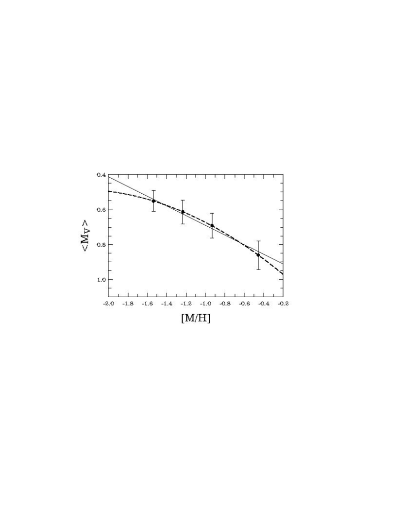
The latter equation provides $M_{V}=0.60$ mag at ${\rm[Fe/H]}=-1.5$ (assuming ${\rm[\alpha/Fe]}\simeq 0.3$; e.g., Carney 1996), in very good agreement with the favored values in Chaboyer (1999) and Cacciari (2003)—thus supporting a distance modulus for the LMC of $(m-M)_{0}=18.47$ mag.

Figure 14.— Predicted correlation between average RRL $V$-band absolute magnitude and metallicity. Each of the four datapoints represents the average magnitude over the full sample of simulations for that metallicity. The “error bars” actually indicate the standard deviation of the mean. The full and dashed lines show equations (11) and (12), respectively.

To close, we note that the present models, which cover only a modest range in metallicities, do not provide useful input regarding the question of whether the $M_{V}-{\rm[M/H]}$ relation is better described by a parabola or by two straight lines (Bono et al. 2003). To illustrate this, we show, in Figure 14, the average RRL magnitudes for each metallicity value considered, along with equations (11) and (12). Note that the “error bars” actually represent the standard deviation of the mean over the full set of RRL stars in the simulations for each [M/H] value.

7. Conclusions

We have presented RRL PL relations in the bandpasses of the Johnsons-Cousins-Glass $UBVRIJHK$ system. While in the case of the Cepheids the existence of a PL relation is a necessary consequence of the large range in luminosities encompassed by these variables, in the case of RRL stars useful PL relations are instead primarily due to the occasional presence of a large range in bolometric corrections when going from the blue to the red edge of the RRL instability strip. This leads to particularly useful PL relations in $IJHK$, where the effects of luminosity and temperature conspire to produce tight relations. In bluer passbands, on the other hand, the effects of luminosity do not reinforce those of temperature, leading to the presence of large scatter in the relations and to a stronger dependence on evolutionary effects. We provide a detailed tabulation of our derived slopes and zero points for four different metallicities and covering virtually the whole range in HB morphology, from very red to very blue, fully taking into account, for the first time, the detailed effects of evolution away from the zero-age HB upon the derived PL relations in all of the $UBVRIJHK$ passbands. We also provide “average” PL relations in $IJHK$, for applications in cases where the HB type is not known a priori; as well as a new calibration of the $M_{V}-{\rm[Fe/H]}$ relation. In Paper II, we will provide comparisons between these results and the observations, particularly in $I$, where we expect our new calibration to be especially useful due to the wide availability and ease of observations in this filter, in comparison with $JHK$.

References

• (1) Bono, G., Caputo, F., Castellani, V., Marconi, M., & Storm, J., 2001, MNRAS, 326, 1183
• (2) Bono, G., Caputo, F., Castellani, V., Marconi, M., Storm, J., & Degl’Innocenti, S. 2003, MNRAS, 344, 1097
• (3) Cacciari, C. 2003, in New Horizons in Globular Cluster Astronomy, ASP Conf. Ser., Vol. 296, ed. G. Piotto, G. Meylan, S. G. Djorgovski, & M. Riello (San Francisco: ASP), 329
• (4) Caputo, F., De Stefanis, P., Paez, E., & Quarta, M. L. 1987, A&AS, 68, 119
• (5) Caputo, F., Marconi, M., & Santolamazza, P. 1998, MNRAS, 293, 364
• (6) Carney, B. W. 1996, PASP, 108, 900
• (7) Castellani, V., Chieffi, A., & Pulone, L. 1991, ApJS, 76, 911
• (8) Catelan, M. 1993, A&AS, 98, 547
• (9) Catelan, M. 2004a, ApJ, 600, 409
• (10) Catelan, M. 2004b, in Variable Stars in the Local Group, ASP Conf. Ser., Vol. 310, ed. D. W. Kurtz & K. Pollard (San Francisco: ASP), in press (astro-ph/0310159)
• (11) Catelan, M., Borissova, J., Sweigart, A. V., & Spassova, N. 1998, ApJ, 494, 265
• (12) Chaboyer, B. 1999, in Post-Hipparcos Cosmic Candles, ed. A. Heck & F. Caputo (Dordrecht: Kluwer), 111
• (13) Clem, J. L., VandenBerg, D. A., Grundahl, F., & Bell, R. A. 2004, AJ, 127, 1227
• (14) Davidge, T. J., & Courteau, S. 1999, AJ, 117, 1297
• (15) Demarque, P., Zinn, R., Lee, Y.-W., & Yi, S. 2000, AJ, 119, 1398
• (16) Ferraro, F. R., Paltrinieri, B., Fusi Pecci, F., Rood, R. T., & Dorman, B. 1998, ApJ, 500, 311
• (17) Girardi, L., Bertelli, G., Bressan, A., Chiosi, C., Groenewegen, M. A. T., Marigo, P., Salasnich, B., & Weiss, A. 2002, A&A, 391, 195
• (18) Isobe, T., Feigelson, E. D., Akritas, M. G., & Babu, G. J. 1990, ApJ, 364, 104
• (19) Leavitt, H. S. 1912, Harvard Circular, 173 (reported by E. C. Pickering)
• (20) Longmore, A. J., Fernley, J. A., & Jameson, R. F. 1986, MNRAS, 220, 279
• (21) Pritzl, B. J., Smith, H. A., Catelan, M., & Sweigart, A. V. 2002, AJ, 124, 949
• (22) Salaris, M., Chieffi, A., & Straniero, O. 1993, ApJ, 414, 580
• (23) Stellingwerf, R. F. 1984, ApJ, 277, 322
• (24) Sweigart, A. V., & Catelan, M. 1998, ApJ, 501, L63
• (25) Tanvir, N. R. 1999, in Post-Hipparcos Cosmic Candles, ed. A. Heck & F. Caputo (Kluwer: Dordrecht), 17
• (26) van Albada, T. S., & Baker, N. 1971, ApJ, 169, 311
• (27) van Albada, T. S., & Baker, N. 1973, ApJ, 185, 477
• (28) VandenBerg, D. A., Swenson, F. J., Rogers, F. J., Iglesias, C. A., & Alexander, D. R. 2000, ApJ, 532, 430