An Enlarged Cosmic Shear Survey with the William Herschel Telescope

Abstract

We report the results of a cosmic shear survey using the 4.2m William Herschel Telescope on La Palma, to a depth of $R=25.8$ ($z\approx 0.8$), over 4 square degrees. The shear correlation functions are measured on scales from $1^{\prime}$ to $15^{\prime}$, and are used to constrain cosmological parameters. We ensure that our measurements are free from instrumental systematics by performing a series of tests, including a decomposition of the signal into $E$- and $B$-modes. We also reanalyse the data independently, using the shear measurement pipeline developed for the COMBO-17 survey. This confirms our results and also highlights various effects introduced by different implementations of the basic “KSB” shear measurement method. We find that the normalisation of the matter power spectrum on 8 $h^{-1}$Mpc scales is $\sigma_{8}=(1.02\pm 0.15)(0.3/\Omega_{m})^{0.5}$, where the 68%CL error includes noise, sample variance, covariance between angular scales, systematic effects, redshift uncertainty and marginalisation over other parameters. We compare these results with other cosmic shear surveys and with recent constraints from the WMAP experiment.

1 Introduction

Weak gravitational lensing by large-scale structure, or “cosmic shear”, has emerged as a powerful cosmological probe, as it is directly sensitive to foreground mass (for reviews, see Bartelmann & Schneider, 2000; Bernardeau, 1999; Mellier, 1999; Refregier, 2003; Wittman, 2002). A measurement of cosmic shear is therefore closely tied to cosmological theories, which are principally concerned with the distribution of dark matter. In particular, the systematic biases of this technique are not limited by unknown physics such as biasing (Dekel & Lahav, 1999; Gray et al., 2002; Hoekstra et al., 2002b; Smith et al., 2003; Weinberg et al., 2000) or the mass-temperature relation for X-ray selected galaxy clusters (Huterer & White, 2003; Pierpaoli, Scott & White, 2001; Viana, Nichol & Liddle, 2002).

Cosmic shear surveys are rapidly growing in size and precision (Bacon et al., 2003; Brown et al., 2003; Hamana et al., 2003; Hoekstra et al., 2002a; Jarvis et al., 2003; Refregier Rhodes, & Groth, 2002; Rhodes, Refregier & Groth, 2001; Van Waerbeke et al., 2002). Cosmological parameter constraints from these surveys are now approaching the precision of other methods.

However, cosmic shear surveys can be subject to several systematic biases of their own. Imperfect telescope tracking, telescope flexure or optical misalignment within the camera, even at a level that is acceptable for most purposes, can artificially distort images and align the shapes of distant galaxies in a way that mimics cosmic shear.

The survey described in this paper represents a culmination of effort at the William Herschel Telescope. We have combined the experience of instrumentalists with detailed image simulations and careful data analysis to control the various sources of systematic error. Our first cosmic shear paper (Bacon, Refregier & Ellis, 2000) reported an initial detection of cosmic shear using a 0.5 square degree survey with the William Herschel Telescope (WHT). The second paper (Bacon et al., 2003) compared the WHT shear signal with an independent measurement using the Keck II telescope, and examined systematics from these two very different instruments. In this paper, we extend our WHT survey to cover 4 square degrees to constrain cosmological parameters, while paying great care in monitoring and correcting systematic effects. We also now test our entire pipeline for shear measurement and cosmological parameter estimation by comparing it to external code, developed independently for the COMBO-17 survey by Brown et al. (2003).

This paper is organised as follows. In §2 we describe our survey strategy and observational parameters. In §3 we present our results and draw constraints upon cosmological parameters. In §4 we test for the absence of any systematic errors. In §5, we present a second set of results obtined via an independent shear measurement pipeline. We conclude in §6.

2 Observations and Data Reduction

We have acquired 4 square degrees of imaging to $R=25.8$ (for a point source at $5\sigma$) with the Prime Focus Imaging Camera (PFIC) of the William Herschel Telescope on La Palma. The median seeing was $0.69\arcsec$ and no exposures had seeing worse than $1\arcsec$. The pixel size is $0.24\arcsec$. As shown in figure 1, pointings were scattered randomly in a pencil-beam survey between galactic latitudes of $30\degr$ and $70\degr$. This was tuned to provide $\sim 1.5$ stars per arcmin², with which we could measure the Point Spread Function (PSF) across each field. The only selection criterion was to avoid foreground stars brighter than $R\approx 11$ in the Digitised Sky Survey or APM (Automated Plate Measuring machine) catalogues.

Cosmic shear statistics have already been presented from the first square degree of this survey in Bacon et al. (2003). That data consisted of eight $8\arcmin\times 16\arcmin$ images and eleven $16\arcmin\times 16\arcmin$ images taken after the addition of a second, identical CCD to the PFIC. During June and August 2002, we observed an additional 41 $16\arcmin\times 16\arcmin$ pointings. When combining statistical measurements from all of these fields, we weight the contribution of the large fields to be twice that of the small fields. This scheme is ideal for measurements on small angular scales, where the large fields do indeed contain twice as many pairs of galaxies as the small fields. The scheme is non-optimal in exploiting the extra signal on large scales contained via additional pairs across different CCDs. However, in general, as both large and small fields were randomly deployed, no bias should result from our weighting scheme.

For each survey field we took four 900s exposures, each dithered by a few arcseconds from the last. This strategy enabled a continual monitoring of astrometric distortions within the telescope, cosmic ray removal, and lower overheads in the event of inclement weather. Data reduction then proceeded for the exposures exactly as in Bacon et al. (2003): see that paper for more details. After bias subtraction and flat fielding, fringing remained in the $R$-band images. This could have been prevented by observing at a shorter wavelength, but at a cost to the observed number density of background sources. To remove this, a fringe frame was compiled from all the exposures in each night. A multiple of this was subtracted from each image which minimised fringing, to a negligible level $<0.05$% of the background noise. The four dithers for each field were then re-aligned (using linear interpolation between adjacent pixels to allow sub-pixel offsets) and stacked (with $3\sigma$-clipping to remove cosmic rays).

Figure 1: The locations of WHT pointings in our deep pencil-beam survey strategy. The galactic latitudes were tuned to provide sufficient foreground stars within each image to successfully model and correct for variations in the PSF.

Objects were located on the final images using hfindpeaks from the imcat package by Kaiser, Squires & Broadhurst (1995, KSB). Following the recommendations of Massey et al. (2001), objects within 10$\arcsec$ of saturated stars or 5$\arcsec$ of the edge of the CCDs were masked and removed. We also removed noisy objects from the catalogue with cuts in size, signal-to-noise and ellipticity of $r_{g}>1\mathrm{~{}pixel}$, $\nu>15$ and $|\varepsilon|<0.5$. This is the same procedure to that adopted in Bacon et al. (2003), and leaves 15.2 galaxies per arcmin² in the final catalogue, with a median magnitude of $23.5\pm 0.2$. According to Cohen et al. (2000) as before, this corresponds to a median source redshift of $z_{s}\simeq 0.80\pm 0.06$.

Galaxies’ observed ellipticities, $\varepsilon$, were formed from combinations of their Gaussian-weighted quadrupole moments, then corrected for convolution with the telescope’s PSF. The shape of the PSF was measured from stars in each image, then interpolated to the positions of galaxies via a polynomial fit within each CCD separately. The order of this polynomial was varied from field to field: it was occasionally raised to fourth order but lowered to second order where possible. This limited spurious power on small scales and particularly around the edges of the field. Even so, an acceptable polynomial fit to the PSF was not always possible. We conservatively discarded 14 fields, all of which were otherwise within specifications, but whose stellar ellipticities remained correlated after correction. More sophisticated PSF fitting methods have recently been suggested by Hoekstra (2004) and Jarvis & Jain (2005). Such techniques may improve the interpolation, and thus increase the number of useable fields, but they have not been investigated here.

The shear susceptibility factor for each galaxy, $P^{\gamma}$, was determined from the higher-order shape moments of the galaxy and the interpolated PSF. The shear susceptibility is a notoriously noisy quantity; in this implementation of KSB, we chose to fit $P^{\gamma}$ with a cubic polynomial as a function of galaxy size, $r_{g}$. We can then form shear estimators for each galaxy, $\gamma=\varepsilon/P^{\gamma}$. We apply a final calibration factor of $(0.85\pm 0.04)^{-1}$ to these shears. This calibration factor was determined by Bacon et al. (2001), using our shear measurement pipeline upon simulated WHT images with a known input signal.

Each set of four dithered exposures were also used to continually monitor astrometric distortions within the telescope. As observed in Bacon et al. (2001), these closely follow the engineering predictions in the PFIC manual of $\gamma_{\mathrm{tangential}}=0$, $\gamma_{\mathrm{radial}}=-8.2\times 10^{-5}r^{2}$ with $r$ measured in arcminutes from the field centre. This affects the shear estimate of an average galaxy in a large exposure by less than $2\times 10^{-3}$. A galaxy in the corner of a large exposure is altered by $1\times 10^{-2}$. Since this is no longer an entirely negligible effect in our enlarged survey, we subtract this distortion from the final shear catalogues using the shear addition and subtraction operators in Bernstein & Jarvis (2002).

The resulting distribution of shear estimators is shown in figure 2. Both components of shear are well-fit by the normalised proabability density function

$$P(\gamma_{i})\approx 0.26\frac{\exp(-x^{2}/0.65^{2})}{(x^{2}+0.27^{2})}~{}.$$ (1)

Extended, Cauchy-like wings are a salient feature of the KSB method, where ellipticity measurements are formed from ratios of (noisy) quadrupole moments.

Figure 2: The distribution of measured shear estimators from all galaxies used in the WHT survey. A fitting function is given in the text. The two components of shear are shown superimposed; their distibutions are indistinguishable. Notice, however, the extended wings typical of the KSB method.

3 Results

3.1 Shear-shear correlation functions

The power spectrum of the weak lensing shear is given by

$$C^{\gamma}_{\ell}~{}=~{}\frac{9}{16}\left(\frac{H_{0}}{c}\right)^{4}\Omega_{m}^{2}\int_{0}^{\chi_{h}}\left[\frac{g(\chi)}{D_{A}(\chi)}\right]^{2}P\left(\frac{\ell}{r},\chi\right)~{}{\rm d}\chi,$$ (2)

where $\chi$ is a comoving distance; $\chi_{h}$ is the horizon distance; $D_{A}(\chi)$ is an angular diameter distance; $g(\chi)$ is the lensing weight function; and $P(k,z)$ is the underlying 3D distribution of mass in the universe. The two-point shear correlations functions can be expressed in terms of the power spectrum as

$$C_{1}(\theta) = \frac{1}{4\pi}\int_{0}^{\infty}C_{\ell}^{\gamma}~{}\big{[}{\rm J}_{0}(\ell\theta)+{\rm J}_{4}(\ell\theta)\big{]}~{}\ell~{}{\rm d}\ell$$ (3)

$$C_{2}(\theta) = \frac{1}{4\pi}\int_{0}^{\infty}C_{\ell}^{\gamma}~{}\big{[}{\rm J}_{0}(\ell\theta)-{\rm J}_{4}(\ell\theta)\big{]}~{}\ell~{}{\rm d}\ell~{}.$$ (4)

These can be measured by averaging over galaxy pairs, as

$$C_{1}(\theta) = \langle~{}\gamma_{1}^{r}(\mn@boldsymbol{r})~{}\gamma_{1}^{r}(\mn@boldsymbol{r}+\mn@boldsymbol{\theta})~{}\rangle$$ (5)

$$C_{2}(\theta) = \langle~{}\gamma_{2}^{r}(\mn@boldsymbol{r})~{}\gamma_{2}^{r}(\mn@boldsymbol{r}+\mn@boldsymbol{\theta})~{}\rangle~{},$$ (6)

where $\theta$ is the separation between the galaxies and the superscript ^r denotes components of shear rotated so that $\gamma_{1}^{r}$ ($\gamma_{2}^{r}$) in the first galaxy points along (at 45$\degr$ from) the vector between the pair. A third shear-shear correlation function can be formed,

$$C_{3}(\theta)~{}=~{}\langle~{}\gamma_{1}^{r}(\mn@boldsymbol{r})~{}\gamma_{2}^{r}(\mn@boldsymbol{r}+\mn@boldsymbol{\theta})~{}\rangle~{}+~{}\langle~{}\gamma_{2}^{r}(\mn@boldsymbol{r})~{}\gamma_{1}^{r}(\mn@boldsymbol{r}+\mn@boldsymbol{\theta})~{}\rangle~{},$$ (7)

for which the parity invariance of the universe requires a zero signal. $C_{3}(\theta)$ can therefore be used as a first test for the presence of systematic errors in our measurement.

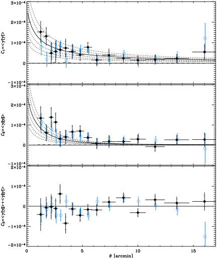
To perform the measurement in practice, we first measure the shear correlation functions in each field, using all galaxy pairs within various $\theta$ bins. To obtain a combined result for the entire survey, we then average the binned values for each field. We find that the measured correlation functions are quite sensitive to changes in the binning scheme. The highly non-Gaussian distribution of shear estimators (see figure 2), plus additional non-Gaussianity introduced by computing correlation functions, means that the inclusion in one bin of a small number of outlying fields can significantly bias measurements. Both the correlation functions and the subsequent constraints on cosmological parameter constraints move within their full 1$\sigma$ statistical error bars. During the averaging, we therefore introduce $3\sigma$-clipping in each bin to remove some outliers, and further $3\sigma$-clipping in $C_{3}(\theta)$ and the star-galaxy cross-correlation functions $C^{\mathrm{S}G}_{1}(\theta)+C^{\mathrm{S}G}_{2}(\theta)$ to eliminate flaws with PSF correction (see §4.2). This leaves between $N_{f}=40$ and $N_{f}=43$ fields used for each angular bin. Our final choice of bin size yields representative central values. The result is shown in figure 3. We shall separately estimate the amount of instability caused by binning, and increase the error upon cosmological parameter constraints accordingly.

Figure 3: Correlation functions of the shear field measured in our 4 square degree WHT survey. The solid data points show our measurement. The inner error bars are for statistical errors only; the outer error bars also include full non-Gaussian sample variance. The blue circles show measurements of our data by the COMBO-17 pipeline, artificially adjusted to correct for its slightly higher source redshift distribution and permit easy comparison. The solid line shows the theoretical prediction for a $\Lambda$CDM model with $\Omega_{m}=0.3$, $\Omega_{\Lambda}$=0.7, $\Gamma=0.21$ and $\sigma_{8}=1.0$, assuming a median source redshift of $z_{s}=0.8$ and using the fitting functions of Smith et al. (2003). The dotted lines show similar theoretical predictions, but with $\sigma_{8}$ ranging from 0.7 (bottom) to 1.2 (top). The dashed lines barely visible above the $x$ axis show the correlation of galaxy shears with the observed PSF anisotropy.

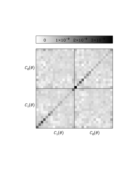
In order to derive any constraints on cosmological parameters, it will also be necessary to know the covariance of $C_{i}(\theta)$ between different angular bins. Our pencil-beam survey strategy with many independent fields makes it easy to measure their covariance matrix

$${\rm cov}[C_{i}(\theta),C_{j}(\vartheta)]~{}\simeq~{}~{}~{}~{}~{}~{}~{}~{}~{}~{}~{}~{}~{}~{}~{}~{}~{}~{}~{}~{}~{}~{}~{}~{}~{}~{}~{}~{}~{}~{}~{}~{}~{}~{}~{}~{}~{}~{}~{}~{}~{}~{}~{}$$

$$\frac{1}{N_{f}^{2}}\sum_{f=1}^{N_{f}}\left[C_{i}^{f}(\theta)-C_{j}(\theta)\right]\left[C_{i}^{f}(\vartheta)-C_{j}(\vartheta)\right]~{},$$ (8)

where the summation is over all fields, and the superscript ^f denotes correlation functions calculated in one field alone. This matrix is depicted in figure 4, and shows the significant covariance, especially between adjacent bins.

Figure 4: Covariance matrix of different angular bins of the shear correlation functions shown in figure 3, from small to large $\theta$, then from small to large $\theta$ again. For example, the bottom-left quarter shows ${\rm cov}[C_{1}(\theta),C_{1}(\vartheta)]$. The diagonal elements within this are the variances in each bin.

3.2 Cosmological parameter constraints

We now use a Maximum Likelihood method to determine the constraints set by our observations upon the cosmological parameters $\Omega_{m}$, the total mass-density of the universe, and $\sigma_{8}$, the normalisation of the matter power spectrum at 8 $h^{-1}$ Mpc. The analysis directly uses the observed correlation functions $C_{1}(\theta)$ and $C_{2}(\theta)$, proceeding as in Bacon et al. (2003), except that theoretical predictions for the non-linear power spectrum are calculated via the updated fitting functions of Smith et al. (2003) rather than those by Peacock & Dodds (1996). This has the effect of lowering our final constraint on $\sigma_{8}\Omega_{m}^{0.5}$ by about $5$%. We use the fitting functions for the linear transfer function suggested by (Bardeen et al., 1986). Note that, although we shall perform an $E/B$ decomposition, we fit $C_{1}$ and $C_{2}$ rather than the $E$ mode signal to avoid degeneracies arising from our survey’s finite size. We will use the $E/B$ decomposition as an a posteriori consistency check for systematics on relevant scales; because of such contamination, we discarded the first and last data points shown in figure 3 (see discussion in §4).

The theoretical correlation functions were first calculated from equation (2) on a 2D grid across the $\Omega_{m}$ vs $\sigma_{8}$ plane. The power spectrum shape parameter was set to $\Gamma=0.21$, consistent with recent observations of clustering in galaxy redshift surveys (Percival et al., 2001; Szalay et al., 2003). The median redshift for source galaxies was fixed to $z_{s}=0.8$ for WHT and $z_{s}=1.0$ for Keck. Errors on these parameters will be propagated separately into our final constraints.

Figure 5: Constraints upon cosmological parameters $\Omega_{m}$ and $\sigma_{8}$, from a maximum-likelihood analysis of our WHT cosmic shear survey data. The 68.3% (solid), 95.4% (dashed) and 99.7% (dotted) confidence limits include statistical errors and non-Gaussian cosmic variance. However, they include neither the calibration of the shear measurement method, nor uncertainty in the source galaxy redshift distribution. These sources of error are considered separately in the text.

Figure 6: Constraints upon cosmological parameters from the Keck cosmic shear survey by Bacon et al. (2003), showing the 68.3%, 95.4% and 99.7% confidence limits as in figure 5. Only one edge of the 99.7% confidence contour is visible inside this parameter range.

We then fitted the observed shear correlation functions $\vec{d}(\theta)$ to the theoretical predictions calculated at the centres of each bin $\vec{t}(\theta)$, computing the log-likelihood function

$$\chi^{2} = \big{(}\vec{d}(\theta)-\vec{t}(\theta,\Omega_{m},\sigma_{8})\big{)}^{T}$$

$$~{}~{}~{}~{}~{}\Big{(}{\rm cov}[C_{i}(\theta),C_{j}(\vartheta)]\Big{)}^{-1}~{}\big{(}\vec{d}(\vartheta)-\vec{t}(\vartheta,\Omega_{m},\sigma_{8})\big{)}$$ (9)

throughout the grid. We thus explore parameter space in this plane, and minimise $\chi^{2}$ to find the best-fit cosmological model. To compute confidence contours, we numerically integrate the likelihood function

$$L(\Omega_{m},\sigma_{8})~{}=~{}e^{-\chi^{2}/2}~{}.$$ (10)

Note that the matrix inversion in equation (9) is unstable, possibly for the same reasons as the binning instability. Since ${\rm cov}[C_{1}(\theta),C_{2}(\theta)]$ is constitent with zero but noisy, we solve this problem in practice by forcing it to zero. The inversion is then well-behaved.

Our constraints on cosmlogical parameters are presented in figure 5, and the constraints from our Keck survey (Bacon et al., 2003) are reproduced in the same format in figure 6. In both cases, the contours show 68.3%, 95.4% and 99.7% confidence limits, including statistical errors and non-Gaussian sample variance. They reveal the well-known degeneracy between $\Omega_{m}$ and $\sigma_{8}$ when using only two-point statistics.

A good fit to the 68.3% confidence level from our WHT data is given by

$$\sigma_{8}\left(\frac{\Omega_{m}}{0.3}\right)^{0.50}=1.02\pm 0.13~{},$$ (11)

while the Keck data is well-fit by

$$\sigma_{8}\left(\frac{\Omega_{m}}{0.3}\right)^{0.52}=1.01\pm 0.19~{},$$ (12)

The multiplication of the respective likelihood functions provides a constraint from a combined survey. Such confidence contours are shown in figure 7, with the 68.3% confidence level well-fit by

$$\sigma_{8}\left(\frac{\Omega_{m}}{0.3}\right)^{0.50}=1.02\pm 0.12~{},$$ (13)

for $0.1<\Omega_{m}<0.7$.

Figure 7: Constraints upon cosmological parameters for the combination of both WHT and Keck surveys, showing the 68.3%, 95.4% and 99.7% confidence limits, as in figure 5.

Note that all of these constraints include only the statistical error and sample variance. We can propagate other sources of error by noting that

$$C_{i}(5^{\prime})\propto\Omega_{m}^{1.46}\sigma_{8}^{2.45}z_{s}^{1.65}\Gamma^{-0.11}(P^{\gamma})^{-2},$$ (14)

where $i=1$ and $2$ and $P^{\gamma}$ is the shear calibration factor, in a fiducial $\Lambda$CDM cosmological model with $\Omega_{m}=0.3$, $\Omega_{\Lambda}$=0.7, $\Gamma=0.21$ and $\sigma_{8}=1.0$. Adding in turn to our constraint (13): a 6% additional binning instability, a 10% source redshift uncertainty, a 15% prior on $\Gamma$, and a 5% shear calibration uncertainty, gives a final 68.3% CL constraint for the combined survey of

$$\sigma_{8}\left(\frac{\Omega_{m}}{0.3}\right)^{0.5}=1.02\pm 0.12\pm 0.06\pm 0.066\pm 0.006\pm 0.04$$ (15)

$$=1.09\pm 0.15~{},~{}~{}~{}~{}~{}~{}~{}~{}~{}~{}~{}~{}~{}~{}~{}~{}~{}~{}~{}~{}~{}~{}~{}~{}~{}~{}~{}~{}~{}~{}~{}~{}~{}~{}~{}~{}~{}~{}~{}~{}~{}~{}~{}~{}~{}~{}~{}~{}~{}~{}~{}~{}~{}$$ (16)

where the various errors have been combined in quadrature on the second line. This result now includes all contributions to the total error budget: (non-Gaussian) statistical noise and sample variance, covariance between different angular scales, binning instability, shear calibration error, source redshift uncertainty, and marginalisation over $\Gamma$.

3.3 Shear variance

For historical reasons, cosmic shear results are often expressed as the variance of the shear field in circular cells on the sky. For a top-hat cell of radius $\theta$, this measure is related to the shear correlation functions by

$$\sigma_{\gamma}^{2} \equiv \langle~{}|\overline{\gamma}|^{2}~{}\rangle~{}~{}=~{}\frac{2}{\pi}\int_{0}^{\infty}C_{\ell}^{\gamma}(\ell)~{}\big{[}{\rm J}_{1}(\ell\theta)\big{]}^{2}~{}\ell~{}{\rm d}\ell$$ (17)

$$\simeq \frac{2}{\theta^{2}}\int_{0}^{\theta}\left[C_{1}(\vartheta)+C_{2}(\vartheta)\right]~{}\mathrm{d}\vartheta~{},$$ (18)

where we have used a small angle approximation involving the Bessel functions. Note that the shear variance is more strongly correlated on different angular scales in this form than they are as correlation functions.

Figure 8: Shear variance in (circular, top-hat) cells, as a function of the radius of the cells. Our results are compared to those from similarly deep surveys by other groups. For ease of comparison, all results have been rescaled as if their median source redshift had been the same (see text). As in figure 3, the theoretical curves are predictions for a $\Lambda$CDM cosmology, with $\Omega_{m}=0.3$, $\Omega_{\Lambda}=0.7$, $\Gamma=0.21$ and $\sigma_{8}$ ranging from 0.7 (bottom) to 1.2 (top).

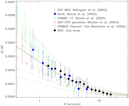
In practice, data is not available on all the scales necessary to perform this integration. The correlation functions have not been calculated on scales smaller than 1$\arcmin$, and are contaminated by systematics on scales smaller than 2$\arcmin$ (see §4). We determine the deficit in the measured values as a function of $\theta$ by extrapolating the data through these scales using the theoretical predictions given by the best-fit cosmological model determined in §3.2. This deficit ($\sim 2\times 10^{-5}$ at $3\arcmin$ and $1\times 10^{-5}$ at $5\arcmin$) is then added back on to our measured data points.

We present our results as the variance of shear in cells, and compare them to those from similarly deep lensing surveys in figure 8. These surveys use data from 8.5 square degree, $z_{s}=0.8$ VIRMOS-Descart survey on the 3.6m CFHT by Van Waerbeke, Mellier & Hoekstra (2005); the 1.25 square degree, $z_{s}=0.85$ COMBO-17 survey on the 2.2m La Silla telescope by Brown et al. (2003); the 0.36 square degree, $z_{s}=0.9$ Medium Deep Survey (MDS) with the Wide Field and Planetary Camera on HST by Refregier Rhodes, & Groth (2002); 0.27 square degrees of random fields observed to $z_{s}=1.0$ in parallel-mode with the Space Telescope Imaging Spectrograph (STIS) on HST by Rhodes et al. (2004); and the 0.6 square degree, $z_{s}=1.0$ pencil-beam survey using the 10m Keck II telescope by Bacon et al. (2003). For ease of comparison between these different surveys, all the results have been scaled to the values that would have been obtained if their median source redshift had been $z_{s}=0.8$, and using the theoretical prediction that $\sigma_{\gamma}^{2}\propto z_{s}^{1.65}$. Results from deeper surveys are thus shown slightly lower here than in their original papers.

4 Tests for systematic Biases

The validity of any cosmic shear result depends sensitively upon the treatment of systematic errors and the control of observational biases. Almost all systematic effects, whether they be due to a background gradient, astrometric distortions within the telescope or imperfectly corrected PSF anisotropy, act to increase the observed correlations between galaxy shapes. All the effects can mimic cosmic shear and the most important task incumbent upon any weak lensing survey is to prove that its systematics are controlled to a negligible level. As already described in §2, the astrometric distortions in WHT have been corrected for, and the basic data reduction was performed sufficiently carefully to eliminate most biases. In this section, we discuss further tests for other sources of residual systematics.

4.1 E-B decomposition

The correlation functions can be recast in terms of $E$ (gradient) and $B$ (curl) modes of the shear field (Crittenden et al., 2000; Pen et al., 2002). Gravitational lensing is expected to produce only $E$ modes, except for a very low level of $B$ modes due to lens-lens coupling along a line of sight (Schneider et al., 2002). Systematic effects are likely to affect both $E$- and $B$-modes equally. The presence of any non-zero $B$ mode would therefore be a useful indication of contamination from other sources.

$E$- and $B$-modes correspond to patterns within an extended region on the sky. The separation cannot be performed locally, but requires the shear correlation functions to be integrated over a wide range of angular scales. In practice, we cannot perform these integrals exactly because our correlation function data extends only between $\sim 2\arcmin$ and $16\arcmin$. In other words, a shear field measured within a finite aperture can not be uniquely split into distinct $E$- and $B$-mode components: some correction will always be necessary.

We find the frequently-used decomposition into aperture mass $M_{\rm ap}(\theta)$ and $M_{\perp}(\theta)$ modes (Bartelmann & Schneider, 2000) to be particularly unstable with our data. The correlation functions need to be integrated between 0 and $2\theta$, with a lot of weight placed upon their values at small angular scales. Since these are changing rapidly, the end result becomes even more sensitive to the bin spacing. Furthermore, our measured correlation functions are least reliable at small separations. This is likely to be the case in any real data because of small-scale effects like overlapping galaxy isophotes. Since data from these small scales need to be included in all subsequent integrals, any bias there would adversely affect the aperture mass on all scales.

Figure 9: $E$-$B$ decomposition of the shear field observed in our WHT survey. The points show the measured $E$ (tangential) modes of the shear field. As in figure 3, the theoretical curves are predictions for a $\Lambda$CDM cosmology, with $\Omega_{m}=0.3$, $\Omega_{\Lambda}=0.7$, $\Gamma=0.21$ and $\sigma_{8}$ ranging from 0.7 (bottom) to 1.2 (top). The dashed line line shows our measured $B$-mode (curl) signal, and the shaded region shows its 1$\sigma$ error bar. In the absence of systematics, the $B$-mode should be consistent with zero.

We therefore prefer another method for $E/B$ decomposition. Following Crittenden et al. (2000), we calculate

$$C_{E}(\theta)\equiv C_{1}(\theta)+2\int_{\theta}^{\infty}\left(1-\frac{3\theta^{2}}{\vartheta^{2}}\right)\frac{C_{1}(\vartheta)-C_{2}(\vartheta)}{\vartheta}~{}\mathrm{d}\vartheta~{},$$ (19)

which contains only the $E$-mode signal and

$$C_{B}(\theta)\equiv C_{2}(\theta)-2\int_{\theta}^{\infty}\left(1-\frac{3\theta^{2}}{\vartheta^{2}}\right)\frac{C_{1}(\vartheta)-C_{2}(\vartheta)}{\vartheta}~{}\mathrm{d}\vartheta~{},$$ (20)

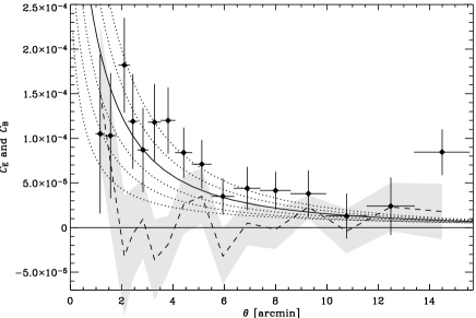
which contains only the $B$-mode signal. These can be calculated using data exclusively from scales larger than $\theta$. A correction will still need to be made for absence of data on scales larger than $16\arcmin$, but this is in a regime where the expected signal (and the necessary correction) is small. As can be seen from the above equation, a function of $\theta$ (not only a constant of integration) must be added to $C_{E}(\theta)$ and subtracted from $C_{B}(\theta)$ (c.f. Pen et al., 2002). We calculate this function by using theoretical predictions for the best-fit cosmological model (as determined in §3.2) to extrapolate our data to infinity. The size of this correction is approximately one third of the size of the measured $E$-mode signal. The correction is 2.4$\times 10^{-5}$ at $5\arcmin$ and 1.5$\times 10^{-5}$ at $10\arcmin$.

An $E$/$B$ decomposition of our data is shown in figure 9. On scales $1.7^{\prime}<\theta<15^{\prime}$, we find a $B$-mode signal consistent with zero, confirming the absence of systematics on these scales. Note that because of the extra uncertainty introduced by this additive function, we have not used the derived $E$-mode signal to fit cosmological parameters. We instead direcly fit the measurements of $C_{1}$ and $C_{2}$ on those scales deemed free of systematic errors only (see §3.2).

4.2 PSF correction

The WHT PSF over long exposures can be quite anisotropic, with a mean stellar ellipticity of $0.051\pm 0.28$, where the error quoted is the rms stellar ellipticity within one field, averaged over all fields. Application of KSB reduces this to $0.0056\pm 0.0012$. Figure 10 shows the full correlation functions

$$C_{i}^{\rm SS}~{}\equiv~{}\langle~{}e^{*}_{i}~{}e^{*}_{i}~{}\rangle~{},$$ (21)

where $i=\{1,2\}$. Application of the KSB method has successfully reduced these by four orders of magnitude. Note that these are correlations of ellipticity rather than shear, and therefore exhibit a different overall normalisation that is connected to the shear susceptibility factor. The elimination of stellar anisotropy is also a slightly different problem than the challenging correction of galaxy shapes, where the interpolation of the PSF is critical, and the size of the weight function $r_{g}$ may be different.

Figure 10: Correlation functions of stellar ellipticities before (dashed line) and after correction (solid points). The shaded region shows the size of 1$\sigma$ errors on the pre-correction correlation functions. Application of the KSB method has successfully reduced these by about four orders of magnitude.

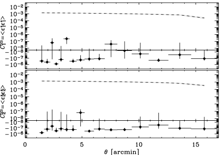
The correction of galaxy shapes for the PSF anisotropy can be tested using cross-correlation functions between corrected shears $\gamma_{i}$ from galaxies and stellar ellipticity $e^{*}_{i}$ before correction,

$$C_{i}^{\rm SG}~{}\equiv~{}\frac{\langle~{}\gamma_{i}~{}e^{*}_{i}~{}\rangle^{2}}{\langle~{}e^{*}_{i}~{}e^{*}_{i}~{}\rangle~{}},$$ (22)

where $i=\{1,2\}$. These cross-correlation functions are shown as dashed line in the top two panels of figure 3, and is consistent with zero on all scales. Note that PSF correction residuals would also have appeared as $B$-modes in figure 9, which are in fact consistent with zero.

Uncertainties still remain in the KSB method about the overall calibration of shear estimators after PSF correction (e.g. Bernstein & Jarvis, 2002; Van Waerbeke et al., 2002). Detailed image simulations by Bacon et al. (2001) or Erben et al. (2001) have been used to study these issues. Bacon et al. (2001) found that, with our survey and telescope parameters, our implementation of KSB requires a constant calibration factor of $(0.85\pm 0.04)^{-1}$ to be applied to all calculated shear estimators.

4.3 Shear as a function of CCD position

Problems with read noise or charge transfer efficiency on the CCD, or telescope flexure and vibration, could cause the measured shear to vary as a function of position on the chip, even when averaged over many separate fields. Figure 11 shows plots of shear as a function of $x$ and $y$. Figure 12 shows plots of shear as a function of $r$. Both are consistent with zero, as desired.

Figure 11: Galaxy shears as a function of position on the WHT CCD, averaged over all the fields used in our survey. That this is consistent with zero everywhere demonstrates an absence of systematics concerning CCD readout, telescope vibration and tracking.

Figure 12: The radial and “curl” components of galaxy shears as a function of distance from the field centre/optical axis, averaged over all the fields used in our survey. That this is conststent with zero on all scales demonstrates an absence of systematics concerning alt-az tracking, and the successful correction of astrometric distortions within the telescope, whose expected behaviour is purely radial (see §2).

Figure 13: Left panels: The shear susceptibility factor $P^{\gamma}$ for all galaxies, as a function of their size $r_{g}$, with different options for the signal-to-noise cut in the catalogue. The greyscale shows the number density of galaxies throughout the parameter space, calculated by the COMBO-17 pipeline. The WHT pipeline produces results almost identical to the top-left panel. In practice the fit is performed on galaxies for one image at a time, and is therefore more noisy; the fit to all galaxies here is shown merely to guide the eye. The fit in the top panel is reproduced as a dashed line in the bottom panel. When the COMBO-17 pipeline uses a signal to noise cut of $\nu>5$, the population ensemble’s average shear susceptibility is raised. Middle panels: A comparison of the shear estimators derived via the WHT and the COMBO-17 shear measurement pipelines. Only subsequently matched galaxies are included in this plot, and the WHT pipeline always uses a signal to noise cut to the catalogue of $\nu>15$, so all galaxies shown are brighter than that. Consistent results are obtained in the top panel, where the COMBO-17 pipeline also uses a cut of $\nu>15$. The unbiased, 1% dispersion of individual values is merely due to the different interpolation of the PSF across individual fields. When the COMBO-17 pipeline uses a signal to noise cut of $\nu>5$, the shear estimators of all galaxies are lowered, including these bright ones. Right panels: Constraints upon cosmological parameters $\Omega_{m}$ and $\sigma_{8}$, from a maximum-likelihood analysis of shears measured with the COMBO-17 pipeline, using different options for the signal-to-noise cut. The 68.3%, 95.4% and 99.7% confidence contours are shown.

The mean components of shear across the entire CCD are $\langle\gamma_{1}\rangle=(1.1\pm 7.1)\times 10^{-4}$ and $\langle\gamma_{2}\rangle=(15.6\pm 7.0)\times 10^{-4}$. The rms shear within the survey is $\sigma_{\gamma_{1}}=0.293$ and $\sigma_{\gamma_{2}}=0.292$, or $\sigma_{|\gamma|}=\langle|\gamma|^{2}\rangle^{1/2}=0.413$. (Note that our shear measurement pipeline includes a catalogue cut at $|\varepsilon|<0.5$). The main, and irreducible, component of this dispersion comes from the intrinsic ellipticities of source galaxies. From other work performed with high resolution and high S/N space-based data (Rhodes et al., 2004; Refregier Rhodes, & Groth, 2002) and simulated images (Massey et al., 2004), we estimate a fundamental lower limit for $\sigma_{|\gamma|}$ around $0.30$.

5 An independent analysis

Our measurement of $\sigma_{8}$ is at the relatively high end of the distribution of published cosmic shear results. Compared to equivalently deep surveys, it is most different from that published by the COMBO-17 survey by Brown et al. (2003), who obtain $\sigma_{8}(\Omega_{m}/0.3)^{0.49}=0.72^{+0.08}_{-0.09}$. We have therefore re-analysed our WHT data using several variations of the COMBO-17 pipeline to determine the extent to which this disagreement might arise from technical differences in the pipelines.

There are four main differences between the COMBO-17 and the WHT pipelines. In the COMBO-17 pipeline:

• the PSF was interpolated across every field via third-order polynomials in $x$ and $y$, so the correction may be different in idividual cases. Data was excluded on all scales for any fields with problematic PSF correction,

• a less stringent signal-to-noise cut was applied. All galaxies with $\nu>5$ were included, rasising the overall number density to 19.8. Every galaxy was still given the same weight when their shears were combined,

• galaxy pairs were not included if the galaxies lay on different CCDs. This will lower the signal-to-noise on large scales but may remove some bias if the chips are imperfectly aligned on the focal plane,

• no correction was made for astrometric distortions in the telescope. This will spuriously increase the signal on large scales, where galaxies are a long way from the telescope axis,

• independently-developed code was used to calculate theoretical models and to fit cosmological parameters to the data.

5.1 Shear measurement

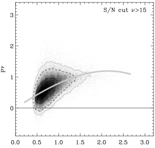
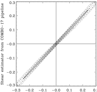
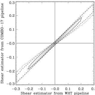
The first two changes are relevant in the creation of a shear catalogue. Differences in the PSF interpolation introduce a $\sim$1% rms dispersion between shear values measured by the WHT or COMBO-17 pipelines (see the top-middle panel in figure 13). This small difference can be explained by the uncertain nature of any interpolation between sparsely sampled data points. The lower-order fit in the WHT method typically produces smoother, and therefore perhaps more reasonable behaviour in regions of the images that are devoid of stars. However, neither method appears to bias the shear estimators or resulting constraints on cosmological parameters.

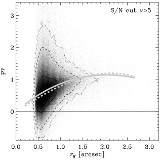
Of greater importance are the $\nu>15$ or $\nu>5$ catalogue cuts in signal-to-noise. Very faint galaxies were discarded in our original analysis of WHT images, and the simulated images of Bacon et al. (2001), because of residual correlation found between the galaxy and stellar ellipticities after correction. Such correlations were not observed in the COMBO-17 data, so the cut was lowered. A possible explanation is the absence of CCD fringing in the COMBO-17 data. Uncorrected fringing in WHT images would alter the shapes of those galaxies at a flux level comparable to the fringing via an additive process rather than a convolution or multiplication. This would not have been corrected, so the galaxies would have simply been discarded. Brighter galaxies that appear in both the WHT-pipeline and COMBO-17 pipeline have identical estimates of $P^{\gamma}$, since both are calculated by hfindpeaks. However, these values are noisy. Both pipelines regard galaxies as a population ensemble, for which it is possible to average over noise by fitting a global shear susceptibility factor.

Theoretically, the susceptibility factor of a galaxy shear is expected to vary as a function of its radial profile, size and ellipticity; but not as a function of its flux. We therefore fit $P^{\gamma}=P^{\gamma}(r_{g})$, as shown in the left-hand panels of figure 13. However, it seems that real faint galaxies do indeed have higher shear susceptibilities than similarly-sized bright galaxies. As shown in the middle panels of figure 13, this raises $P^{\gamma}(r_{g})$, and thus lowers shear esimators by a factor of $0.85^{+0.12}_{-0.5}$. The skewed distribution reflects the overall size distribtuion of galaxies, and arises because this process affects small galaxies more than large ones. The reason for this variation of $P^{\gamma}(\nu)$ is not yet clear: it may be that the morphology distribution of faint galaxies really does contain intrinsically higher shear susceptibilities. Both approaches would be valid in this case, since the fit really has found a suitable average value for the population ensemble of galaxies.

A more worrying alternative would be that the noise in faint galaxies biases $P^{\gamma}$ to higher values, partly because the main $P^{\rm sh}$ component of $P^{\gamma}$ (see Kaiser, Squires & Broadhurst, 1995) is defined to be strictly positive. In this case, it would instead be preferable to fit only the bright galaxies, then apply that susceptibility to faint galaxies of the same size. Either way, the results from the WHT pipeline would be less affected, as the $\nu>15$ cut has been calibrated upon simulated images containing a known signal by Bacon et al. (2001).

A full investigation into this technical issue is beyond the scope of this paper, and it will need further investigation in the future. Other comparative studies, e.g. the Shear TEsting Program (STEP, Heymans et al. in preparation), or the Edinburgh and Bonn pipelines (Heymans et al. in preparation), find that the detailed way in which $P^{\gamma}$ is, or is not, adequately fit may indeed explain a large part of the variation between results from different implementations of KSB. Here, we shall propagate the analysis of shear catalogues from the COMBO-17 pipeline with both $\nu>15$ and $\nu>5$ cuts.

5.2 Cosmological parameter constraints

We find similar instabilities in the production of shear-shear correlation functions with the COMBO-17 pipeline as we found in the WHT pipeline; results are sensitive to binning at the $\sim\pm$7% level. Measurements with the $\nu>5$ as shown as blue circles in figure 3, rescaled by a factor $(0.8/0.9)^{1.65}$ to allow comparison despite the increased source redshift distribtion. Excluding galaxy pairs of different CCDs has increased the size of error bars by up to 50% at large $\theta$, where the number of available galaxy pairs is significantly lower, but the central values move only within their $1\sigma$ error bars. Not correcting for the telescope’s known astrometric distortion has moved the bin at largest scales by a significant amount, but this is not used for parameter fitting anyway. Excluding data on all scales from fields with any residual star-galaxy correlation also has a minimal effect. Each of these differences change the derived constraint on $\sigma_{8}$ by less than 1%.

The main difference in the two analyses is that introduced by the different cuts in signal-to-noise. The inclusion of fainter galaxies increases the median magnitude of the $\nu>5$ population by $0.84\pm 0.4$ magnitudes, leading to a new median redshift of $z_{s}=0.90\pm 0.07$ (Cohen et al. (2000)). The expected cosmic shear signal thus increases (see equation 14) – an effect that is incorporated during the calculation of theoretical models for the fitting of cosmological parameters. Reassuringly, the shear signal measured from faint galaxies is also higher. The final constraints for the COMBO-17 pipeline, using a cut of $\nu>15$ indicate:

$$\sigma_{8}\left(\frac{\Omega_{m}}{0.3}\right)^{0.52}=1.01\pm 0.13~{},$$ (23)

including only statistical errors and, for a cut of $\nu>5$ with the higher assumed source redshift distribution

$$\sigma_{8}\left(\frac{\Omega_{m}}{0.3}\right)^{0.52}=0.98\pm 0.10~{}.$$ (24)

The consistency of these fits, and their agreement with the results from the WHT pipeline is reassuring. They tend to justify the adoption of a global shear susceptibility factor for an ensemble population of galaxies, and verify the validity of the methods for controlling many potential systematic effects in both pipelines.

Our survey probes a wide range of angular scales, and thus excludes small values of $\Omega_{m}<0.25$ (at 68%CL). The preference for large $\Omega_{m}$ comes from the fit to the transfer function by (Bardeen et al., 1986). If we adopt the fit by Eisenstein & Hu (1997), and assume the Hubble parameter $h=0.7$, we effectively apply a different prior on $\Omega_{m}$. In this case, our data excludes $\Omega_{m}>0.55$ (at 68%CL), similar to the result obtained by Van Waerbeke, Mellier & Hoekstra (2005). Using the Eisenstein & Hu (1997) transfer function also lowers our best-fit value for $\sigma_{8}$ around $\Omega_{m}=0.3$ by $\sim$2%.

6 Conclusions

We have measured the weak lensing shear-shear correlation functions in four square degrees of deep $R$-band imaging data from the William Herschel Telescope. Our measurements constrain the amplitude of the mass power spectrum, $\sigma_{8}(\Omega_{m}/0.3)^{0.52}=1.02\pm 0.15$, including all contributions to the total 68%CL error budget: statistical noise, sample variance, an additional estimated error due to binning instabilities from non-Gaussian outliers, covariance between different angular scales, systematic measurement and detection biases, source redshift uncertainty, and marginalisation with priors over other parameters. We have examined our data for contamination by systematic effects using a variety of tests including an $E$-$B$ decomposition. These demonstrate a well-understood and modest contribution to our uncertainties from systematic errors.

Using the pipeline developed for earlier WHT studies, we find our measurement of the normalization of the dark matter power spectrum lies at the relatively high end of the distribution of published values. However, it is still consistent with those from equivalently deep surveys by Refregier Rhodes, & Groth (2002) and (Rhodes et al., 2004). Our results are also consistent at the 1$\sigma$ level with CMB results from the Wilkinson Microwave Anisotropy Probe (WMAP) (Spergel et al., 2003).

The wide distribution of $\sigma_{8}$ constraints from recent cosmic shear surveys understandably casts some aspersion upon their precision. For example, it might be argued that the dispersion largely arises from unknown or poorly-understood systematic effects. For the first time we analyze our dataset with an independent pipeline – that developed for the COMBO-17 data (Brown et al. (2003)). This provides a valuable check on the extent to which dispersion in the published cosmological results, as well as our apparently high normalization, might arise from different techniques, both in constructing shear catalogues and in analysing the shear-shear correlation functions. Reassuringly, we find remarkable concordance between the two pipelines for the same dataset. However, the various differences we have explored, for example in the selection thresholds, seem to be insufficient to reconcile the spread in observed $\sigma_{8}$ values, suggesting that significant differences remain at some level in the actual data themselves.

Uncertainties in the redshift distribution of source galaxies in deep data clearly contribute. It is difficult to determine the precise redshift distribution of galaxies after excluding those smaller than a fixed apparent size. We have been conservative in this analysis and, as seen in equation (15), source redshift uncertainty is already a major component of our total error budget. The resolution of such issues will require extensive spectroscopic follow-up and more complete image simulations. Such advances are essential if the potential of the next generation of cosmic shear surveys is to be fully realised.

Finally, we note that most recent cosmic shear results remain discrepant at the $3\sigma$ level with measurements derived from the abundance of X-ray selected cluster samples based on an observational rather than theoretical mass-temperature relation (Borgani et al., 2001; Seljak, 2001; Reiprich & Böhringer, 2002; Viana, Nichol & Liddle, 2002). These suggest $\sigma_{8}\approx 0.75$. Amara & Refregier (2004) concluded that even extreme non-Gaussianity in the mass distribution would be insufficient to explain this discrepancy, because the two techniques probe similar mass scales. Further studies are therefore needed in both the cluster method, to understand the difference between the observed mass-temperature relation and that found in numerical simulations; and in the weak lensing method, to construct more reliable and better calibrated shear measurement methods. Such consistency checks will represent a crucial verification of the standard $\Lambda$CDM paradigm, so resolving this issue is of paramount importance.

References

- Amara & Refregier (2004) Amara A. & Refregier A., 2004, MNRAS submitted. astro-ph/0310345
- Bacon et al. (2003) Bacon D., Massey R., Refregier A. & Ellis R., 2003, MNRAS, 344, 673
- Bacon, Refregier & Ellis (2000) Bacon D., Refregier A. & Ellis R., 2000, MNRAS, 318, 625
- Bacon et al. (2001) Bacon D., Refregier A., Clowe D. & Ellis R., 2001, MNRAS, 325, 1065
- Bardeen et al. (1986) Bardeen J., Bond J., Kaiser N. & Szalay A., ApJ, 304, 15
- Bartelmann & Schneider (2000) Bartelmann M. & Schneider P., 2000, Phys. Rep., 340, 291
- Bernardeau (1999) Bernardeau F. 1999. Proc. Cargese Summer Sch., Cargese, France, ed. M Lachieze-Rey. astro-ph/9901117
- Bernstein & Jarvis (2002) Bernstein G. & Jarvis M., 2002, ApJ, 123, 583
- Borgani et al. (2001) Borgani S., Rosati P., Tozzi P., Stanford S., Eisenhardt P., Lidman C., Holden B., Della Ceca R., Norman C., Squires G., 2001, ApJ, 561, 13.
- Brown et al. (2003) Brown M., Taylor A., Bacon D., Gray M., Dye S., Meisenheimer K. & Wolf C. MNRAS, 341, 100
- Cohen et al. (2000) Cohen J., Hogg D., Blandford R., Cowie L., Hu E., Songaila A., Shopbell P. & Richberg K., 2000, ApJ, 538, 29
- Crittenden et al. (2000) Crittenden R., Natarajan P., Pen U.-L. & Theuns T., 2000, ApJ, 559, 552
- Dekel & Lahav (1999) Dekel, A. & Lahav, O., 1999, ApJ, 520, 24
- Eisenstein & Hu (1997) Eisenstein D. & Hu W., 1997, ApJ, 511, 5
- Erben et al. (2001) Erben T., van Waerbeke L., Bertin E., Mellier Y. & Schneider P., 2001, A&A, 366, 717
- Gray et al. (2002) Gray M., Taylor A., Meisenheimer K., Dye S., Wolf C. & Thommes E., 2002, ApJ, 568, 141
- Hamana et al. (2003) Hamana T. et al., 2003, ApJ in press, preprint astro-ph/0210450
- Hämmerle et al. (2002) Hämmerle et al., 2002, A&A, 385, 743
- Huterer & White (2003) Huterer & White, 2003, ApJ, 578, L95
- Hoekstra et al. (2002a) Hoekstra H., Yee H., Gladders M., Felipe Barrientos L., Hall P. & Infante, L., 2002a, ApJ, 572, 55
- Hoekstra et al. (2002b) Hoekstra H., van Waerbeke L., Gladders M., Mellier Y. & Yee H., 2002b, ApJ, 577, 604
- Hoekstra (2004) Hoekstra H., 2004, MNRAS, 347, 1337
- Jarvis et al. (2003) Jarvis M., Bernstein G., Fisher P., Smith D., Jain B. et al., 2003, AJ, 125, 1014
- Jarvis & Jain (2005) Jarvis M. & Jain B., 2005, ApJ submitted, preprint astro-ph/0412234
- Kaiser, Squires & Broadhurst (1995) Kaiser N., Squires G. & Broadhurst T., 1995, ApJ, 449, 460
- Massey et al. (2001) Massey R., Bacon D., Refregier A. & Ellis R., 2001, ASP conf. ser. Vol 283, p.193., eds. T. Shanks & N. Metcalfe.
- Massey et al. (2004) Massey R. et al., 2004, AJ in press, preprint astro-ph/0304418
- Massey et al. (2004) Massey R., Refregier A., Conselice C. & Bacon D., 2004, MNRAS, 348, 214
- Mellier (1999) Mellier Y., 1999, ARA&A, 37, 127
- Peacock & Dodds (1996) Peacock J. & Dodds S., 1996, MNRAS, 280, 19
- Percival et al. (2001) Percival W. et al., 2001, MNRAS, 327, 1297
- Pen et al. (2002) Pen U., Van Waerbeke L. & Mellier Y., 2002, ApJ, 567, 31
- Pierpaoli, Scott & White (2001) Pierpaoli E., Scott D. & White M., 2001, MNRAS, 325, 77
- Reiprich & Böhringer (2002) Reiprich T. & Böhringer H., 2002, ApJ, 567, 716
- Refregier (2003) Refregier A., 2003, ARA&A, 41, 645
- Refregier Rhodes, & Groth (2002) Refregier A., Rhodes, J. & Groth E., 2002, ApJL, 572, 131
- Rhodes, Refregier & Groth (2001) Rhodes J., Refregier A. & Groth E., 2001, ApJL, 552, 85
- Rhodes et al. (2004) Rhodes J., Refregier A., Collins N., Gardner J., Groth E. & Hill R., 2004, ApJ in press. astro-ph/0312283
- Seljak (2001) Seljak U., 2001, MNRAS, 337, 769
- Schneider et al. (2002) Schneider P., van Waerbeke, L. & Mellier Y., 2002, A&A, 389, 729
- Smith et al. (2003) Smith G., Edge A., Eke V., Nichol R., Smail I. & Kneib J.-P., 2003, AJ, 590, L79
- Smith et al. (2003) Smith R., Peacock J., Jenkins A., White S., Frenk C., Pearce F., Thomas P., Efstathiou G. & Couchmann H., 2003, MNRAS, 341, 1311
- Spergel et al. (2003) Spergel D. et al. 2003, ApJS, 148, 175
- Szalay et al. (2003) Szalay A. et al. 2003, ApJ, 591, 1
- Van Waerbeke et al. (2001) van Waerbeke L. et al., 2001, A&A, 374, 757
- Van Waerbeke et al. (2002) van Waerbeke L., Mellier Y., Pelló R., Pen U.-L., McCracken H. & Jain, B., 2002, A&A, 393, 369
- Van Waerbeke, Mellier & Hoekstra (2005) van Waerbeke L., Mellier Y. & Hoekstra H., 2005, A&A submitted, preprint astro-ph/0406468
- Viana, Nichol & Liddle (2002) Viana P., Nichol R. & Liddle A., 2002, ApJ, 569,75
- Weinberg et al. (2000) Weinberg D., Davé R., Katz N. & Hernquist L., 2003, ApJ submitted, preprint astro-ph/0212356
- Wittman (2002) Wittman D. 2002. Dark Matter and Gravitational Lensing, LNP Top. Vol., eds. F. Courbin, D. Minniti. Springer-Verlag. astro-ph/0208063