Linear Temperature-Mass relation and Local virial relation: Two hypotheses for self-gravitating systems

Abstract

We propose two hypotheses which characterize the quasi-equilibrium state that realizes after a cold collapse of self-gravitating system. The first hypothesis is the linear temperature-mass (TM) relation, which yields a characteristic non-Gaussian velocity distribution. The second is the local virial (LV) relation, which, combining the linear TM relation, determines a unique mass density profile as $\rho(r)={\rho}_{0}r^{-4}e^{-r_{0}/r}$. Although this density profile is unphysical in the central region, the region is just inner a few percent around the center of a bound region in cumulative mass, which is beyond the resolution of our numerical simulations. Hence posing two hypotheses is compatible to the numerical simulations for almost the whole region of the virialized bound state. Actually, except for this inner part, this density profile fits well to the data of cold collapse simulations. Two families of spherical and isotropic models, polytropes and King models, are examined from a view point of these two hypotheses. We found that the LV relation imposes a strong constraint on these models: only polytropes with index $n\sim 5$ such as Plummer’s model are compatible with the numerical results characterized by the two hypotheses among these models. King models with the concentration parameter $c\sim 2$ violate the LV relation while they are consistent with the $R^{1/4}$ law for the surface brightness. Hence the above characteristics can serve as a guideline to build up the models for the bound state after a cold collapse, besides the conventional criteria concerning the asymptotic behavior.

I Introduction

Collisionless self-gravitating systems (SGS) eventually settle down to a quasi-equilibrium state through the phase mixing and the violent relaxation processes under the potential oscillationLynden67 . This quasi-equilibrium state is a prototype of the astronomical objects such as galaxies and clusters of galaxies. These objects often show universal profiles in various aspects.

It would be true that the energy distribution function and the mass density distribution function are quite appropriate to characterize SGS, and actually many studies have been done from this viewpoint. For example, the density profile is found to be $\rho\propto r^{-4}$ in spherical and cold collapses, i.e., collapses with small initial virial ratio Henon64 ; Albada82 and $\rho\propto r^{-3}-r^{-4}$ in the cluster-pair merging processesMerrall03 .

On the other hand, the velocity distribution function has not fully been examined so far despite its importance ; anisotropy of velocity dispersion or lower moments of velocity distributions with respect to the deviations from Gaussian distributions have been mainly examined (e.g. Binney82 ; Gerhard93 ). However, the full velocity distribution function plays an important role in identifying the quasi-equilibrium state, which should be properly characterized by the whole phase-space probability functions. Merrall et al. numerically showed that the velocity distributions in the central regions of the bound particles become Gaussian, when the bound particles are well relaxed Merrall03 . However, since SGS are manifestly non-additive systems Nakamichi04 , the ordinary Gaussian distribution would not be expected for the whole bound particles. Moreover, such non-Gaussian velocity distributions would be firmly connected with the density profile characteristic to SGS Gerhard93 ; Kazantzidis04 .

Recently, we have simulated self-gravitating N-body systems by utilizing the leap-frog symplectic integrator on GRAPE-5, a special-purpose computer designed to accelerate N-body simulationsGRAPE . The simulations were performed mainly in the case with cold collapse initial conditions. It is certain that the processes may be too simplified to deduce the ultimate nature of actual SGSs, in which merging or tidal effects take place. However, one of our main goals is to establish the universal properties of SGS through the violent relaxation process, i.e. the relaxation through the oscillation of gravitational potential. This process is rather common in actual SGSs such as galaxies and dark matters. In this context, the cold collapse is considered to be a typical case which causes the violent relaxation. Hence it is meaningful to examine the cold collapse as a first step.

When the system experiences violent gravitational processes such as a cold collapse and a cluster-pair collision, we obtained a universal velocity distribution profile expressed as the democratic (=equally weighted) superposition of Gaussian distributions of various temperatures(DT distribution hereafter) in which the local temperature $T(r)$ is defined using the local velocity variance $\langle v^{2}\rangle$ as $T(r):=m\langle v^{2}\rangle(r)/3k_{B}$, where $m$ is the particle mass Osamu04 . Moreover, we have found that the locally defined temperature linearly falls down in the intermediate cluster region outside the central part, provided it is described against the cumulative mass $M_{r}$, i.e., $dT/dM_{r}=const.$ This fact is consistent with the appearance of DT distributions.

Furthermore to the linear TM relation, we have also obtained another peculiar fact that the LV relation between the locally defined potential energy and kinetic energy holds except for the weak fluctuations. More precisely, the local temperature $T(r)$ is proportional to the local potential $\Phi(r)$, with constant proportionality $6k_{B}T(r)=-m\Phi(r)$ for a wide class of cold collapse simulations. It was originally pointed out by Eddington that Plummer’s model satisfies this condition exactly Eddington16 . Moreover it was also pointed out that Plummer’s model can be extended to the anisotropic model of a stellar system satisfing the LV relation Evans05 . We found that the bound region, i.e., the region composed of the bound particles keeps this relation quite well at least during the time interval much longer than the initial crossing time. This is a prominent correlation in the phase space distribution function, and also constructs another backbone character of SGS after a cold collapse.

In sec.II and III, we will show that the above two hypotheses for SGS are supported by the results of a variety of cold collapse simulations. Then in sec.IV, combining the two hypotheses, i.e., the linear TM relation and the LV relation, we obtain a unique density profile $\rho(r)=\rho_{0}(r/r_{0})^{-4}e^{-r_{0}/r}$ which asymptotically behaves as $\rho\propto r^{-4}$. Justification of this density profile will also be discussed. In sec.V, we will ascertain that the above two hypotheses can arise even in the collisionless quasi-equilibrium state, where the region inside a half-mass radius is not yet under the effect of two-body relaxation. In sec.VI the above two hypotheses will be explored in two typical collisionless static models with spherical configuration and isotropic velocity dispersions; polytropes and King models. Sec.VII is devoted to the summaries and conclusions of this paper.

II Linear TM relation

Let us now further consider the linear TM relation. In our recent work Osamu04 , we have examined the velocity distribution function of collisionless SGS after a cold collapse in numerical N-body calculations. According to this work, immediately after a cold collapse, well-relaxed and almost spherical-symmetric bound state is formed. In order to examine the local property, we use the cumulative mass $M_{r}$ within the radius $r$, i.e., $M_{r}:=4\pi\int_{0}^{r}dr^{\prime}r^{\prime 2}\rho(r^{\prime})$ as a measure of the radial distance from the cluster center, which is defined as the position of the potential minimum. In our numerical simulation, we divide the whole system into several concentric shells with equal width in the coordinate $M_{r}$ and consider the averaged quantities within each shell as local variables.

In our simulation, particles in the outermost region, which includes $20\%$ of the total mass, escape almost freely just after the cold collapse and are irrelevant to the quasi-equilibrium state. Therefore we concentrate on the local temperature within the inner region initially including $80\%$ of the total mass. More precisely, we define the bound particles as the particles inside the $M_{r}$, at which the local temperature $T(M_{r})$ takes the minimum value. Hereafter, we pay our attention to the bound region composed of these bound particles. In the central part of this region, the two-body relaxation proceeds and the particles evaporate toward outside. Moreover, in this central region, the effect of cutoff $\epsilon$ proposed in numerical simulations cannot be ignored completely. Discarding this part from the bound region, we found, that the local velocity variance, i.e., the local temperature linearly decreases to zero in the coordinate $M_{r}$,

$$\langle v^{2}\rangle(r)=\frac{3k_{B}T}{m}=c(M_{tot}(t)-M_{r}),$$ (1)

where $c$ is a positive constant and $M_{tot}(t)$ is the total mass of the bound particles at $t$. $M_{tot}(t)$ is initially equal to $80\%$ of the total mass but is gradually diminished, as several particles evaporate from the bound state.

Here we examined the deviation of TM relation from the linear relation (1) for a variety of simulations of cold collapse. For the estimate of the deviation, we first take the time-average for the velocity dispersion at each shell to derive the time-averaged $\langle v^{2}\rangle$-mass relation. Then we linearly fit it as (1) to derive $\langle v^{2}\rangle_{fit}$ and subtract it from $\langle v^{2}\rangle$. In Fig.1, the deviation normalized by $\langle v^{2}\rangle$ at the half mass radius are depicted for several simulations with total particle’s number $N=5000$. The deviations are very small and are less than 10 percent at each $M_{r}$ for all of the simulations we examined. Hence, this result is quite robust against initial conditions with $N=5000$ provided the collapse is cold. Even for the case of cluster-pair collision, this linear relation is widely obtained. We also examined the $N$ dependence of the linear TM relation for the case with initially homogeneous spherical sphere (Fig.2). As $N$ increases, the particles collapse more and more coherently, which causes a shock region moving slowly outward after a collapse. Although such a shock region enhances the deviation from the linear TM relation, the region within a shock region satisfies the linearity quite well.

Figure 1: A mass dependence of velocity dispersion ($\langle v^{2}(M_{r}/M_{tot})\rangle$) obtained by a typical cold collapse simulation; spherical collapse (SC) and cluster-pair collisions (CC). In the case of SC, $5000$ particles are distributed with a power law density profile ($\rho\propto r^{-a}$) within a sphere of radius $R$ and the initial virial ratio ($\bar{b}_{t}$) is set to be small. In the case of CC, each cluster has the equal number of particles ($2500$) and all particles are homogeneously distributed within a sphere of radius $R$ and is set to be virialized initially. The initial separation of the pair is $6R$ along the $x$ axis. In all of the simulations, softening length $\epsilon=2^{-8}R$ is introduced to reduce the numerical error caused by close encounters. The inset figure shows that locally averaged velocity dispersion is plotted as a function of $M_{r}(t)/M_{tot}(t)$ for SC($\bar{b}_{t}=0,a=0$) as a typical example. Apparent linearity is remarkable. The broken line is the best fit line with $c=9.8G/R$ (Eq.(1)). The open circles represent the time averaged numerical data from $t=5t_{ff}$ and $t=100t_{ff}$, where $t_{ff}$ is the initial free fall time defined as $t_{ff}:=\sqrt{R^{3}/GM_{tot}(0)}$. The deviation from the best fit line ($<v^{2}>_{fit}$) normalized by the velocity dispersion at the half mass is shown for some numerical simulations with different initial conditions. The value of each deviation is under $10\%$.

Figure 2: A mass dependence of velocity dispersion ($\langle v^{2}(M_{r}/M_{tot})\rangle$) obtained by a typical cold collapse simulation SC ($\bar{b}_{t}=0,a=0$) with different particle number $N$. The case with $N=5\times 10^{3},10^{4},5\times 10^{4},10^{5}$ are depicted. The peak appears in the case with $N=5\times 10^{4},10^{5}$ around $M_{r}\sim 0.7M_{tot}$, which represents a shock region.

III Local virial relation

Besides the linear TM relation, there is another characteristic for SGS as we now argue. It is well known that the gravitationally bound system approaches a virialized state satisfying the condition

$$\overline{W}+2\overline{K}=0,$$ (2)

where $\overline{W}$ and $\overline{K}$ are, respectively, the averaged potential energy and kinetic energy of the whole bound system. This is a global relation that holds for the entire system, after the initial coherent motion fades out.

Here we define the locally averaged potential energy and kinetic energy inside the radius $r$, respectively as

$$\overline{W}_{r} := \frac{1}{2}\int_{0}^{r}\Phi(r^{\prime})\rho(r^{\prime})4\pi r^{\prime 2}dr^{\prime},$$ (3)

$$\overline{K}_{r} := \int_{0}^{r}\frac{\langle v^{2}\rangle(r^{\prime})}{2}\rho(r^{\prime})4\pi r^{\prime 2}dr^{\prime},$$ (4)

where $\star(r^{\prime})$ means the local object $\star$ evaluated at $r^{\prime}$.

Then we extend the virial relation (2) locally as

$$\overline{W}_{r}+2\overline{K}_{r}=0,$$ (5)

and examine how precisely this relation is locally attained inside a bound state.

Figure 3: The LV relation for some numerical simulations with N=$5000$. The local virial ratio $b$ is plotted as a function of $M_{r}/M_{tot}$. The initial condition of each simulation is the same as Fig.1. The virial ratios of each shell are time averaged from $t=5t_{ff}$ and $t=100t_{ff}$.

Figure 4: The LV relation for some numerical simulations with different particle number $N$. The local virial ratio $b$ is plotted as a function of $M_{r}/M_{tot}$.The case with $N=5\times 10^{3},10^{4},5\times 10^{4},10^{5}$ are depicted. The initial condition of each simulation is the same as Fig.2. The virial ratios of each shell are time averaged from $t=5t_{ff}$ and $t=100t_{ff}$. The peak appears in the case with $N=5\times 10^{4},10^{5}$ around $M_{r}\sim 0.7M_{tot}$, which represents a shock region.

More precisely, the above relation Eq.(5) is equivalent to the purely local relation

$$2\langle v^{2}\rangle(r)=-\Phi(r),$$ (6)

at each position $r$. Hence, we define the LV ratio

$$b(r):=-2\langle v^{2}\rangle(r)/\Phi(r),$$ (7)

and examine the value of $b(r)$ for each shell. For a wide class of collapses including cluster-pair collision examined in Osamu04 , the value $b(r)$ takes almost unity: it deviates from unity less than 10 percent upward in the intermediate region and a little more downward in the inner and outer region for all of the simulations with $N=5000$(Fig.3). Hence a wide class of cold collapse simulations with $N=5000$ yield the relation (6) quite well. We also examined the N-dependence of the LV relation for the cases in Fig.4. We got the result that the LV relation is affected by the shock as well as the linear TM relation in the case with $N\geq 5\times 10^{4}$,where the LV ratio $b$ takes the peak at the shock region. the value $b$ becomes smaller than unity around the shock region in order to compensate for the enhance at the shock region. However, $b$ oscillates around unity even in such cases, which supports the LV relation in the zeroth order. Hence,this LV relation should be an another characteristic of SGS, and this is our second hypothesis.

IV Density profile

We have explored the two hypotheses of SGS so far, i.e., the linear TM relation Eq.(1) and the LV relation Eq.(6) for the bound cluster. Combining these two relations, we now derive a mass density profile. We simply substitute Eq.(6) into Eq.(1) to obtain $2c(M_{tot}-M_{r})=-\Phi$. Differentiating this with $r$ and using Poisson’s equation, we obtain a differential equation for the mass density $\rho(r)$:

$$\frac{d}{dr}(r^{4}\rho)=\frac{G}{2c}r^{2}\rho,$$ (8)

which admits the unique solution

$$\rho(r)={\rho}_{0}\left(\frac{r_{0}}{r}\right)^{4}e^{-r_{0}/r},$$ (9)

where $r_{0}:=G/2c$ and $\rho_{0}$ is a constant. The cumulative mass $M_{r}$ for this density profile is easily derived as

$$M_{r}=M_{tot}e^{-r_{0}/r},$$ (10)

where $M_{tot}$ is the total mass and is described as

$$M_{tot}=4\pi r_{0}^{3}\rho_{0}.$$ (11)

The central part of this density is unphysical, since it increases with increasing radius $r$ inside $r_{\ast}:=r_{0}/4$. This fact warns that the two hypotheses we proposed are not always justified in the entire region. However, $M_{r}$ inside e $r_{\ast}$ is just

$$M_{r}(r_{\ast})=e^{-4}M_{tot}\sim 0.0183M_{tot},$$ (12)

from (10). Hence this unphysical region is at most 2 percent of the full bound region in cumulative mass.

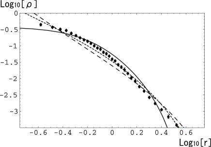
Even if we put a constant density at this inner unphysical region and continuously connect it to the outer analytical solution (9), this inner region is at most three percent of the full bound region in mass (See AppendixA), which is inner than the smallest value of $M_{r}$ for numerical data points in Fig.1 and Fig.3. Hence we can safely neglect this unphysical region. Actually the function (9) fits well to our numerical results (Fig.5). The asymptotic behavior $\rho(r)\propto r^{-4}$ is consistent with previous works Jaffe87 ; makino90 . In sec.VI, we will see how this central part is modified with several collisionless static solutions.

Figure 5: A log-log plot of a typical density profile after a cold collapse. The initial condition of this simulation is the same as SC $(\bar{b}_{t}=0,a=0)$ in Fig.1. The open circles represent the numerical data at $t=100t_{ff}$. The solid line is the density profile (Eq.(9)) with the best fit parameter ($\mbox{Log}_{10}(r_{0}/R)=-1.25$), which corresponds to $M_{r}|_{r=r_{0}}/M_{tot}\sim 0.43$.

V Collisionless or collisional? the properties of the system compatible with the two hypotheses

In the previous section, we numerically showed that the bound system after a cold collapse retains the two hypotheses during a long time interval on average. Here a natural question arises, i.e., do these two characteristics occur just after a cold collapse or are they gradually developed through the two-body relaxation? Now we check this issue by estimating the two-body relaxation time scale $t_{rel}$, which is described as

$$t_{rel}=0.065\frac{{\overline{\langle v^{2}\rangle}^{3/2}}}{{mG^{2}\overline{\langle\rho\rangle}\log\left({1/\epsilon}\right)}},$$ (13)

where $\overline{\langle v^{2}\rangle}$ and $\overline{\langle\rho\rangle}$ are the velocity variance and the density averaged inside the half mass radius, respectively Spitzer87 . Although $t_{rel}$ is a function of time $t$, the value settles down to a constant value $t^{\ast}_{rel}$ when the system stays in a quasi-equilibrium bound state. From the definition of $t_{rel}(t)$, the system inside a half mass radius naively attains two-body relaxation at $t>t^{\ast}_{rel}$. In Table.1, we show the value of $t^{\ast}_{rel}$ for several simulations.

For example, because of the high concentration of the bound particles just after a collapse, $t^{\ast}_{rel}$ becomes very short in the case with a cold collapse from a homogeneous sphere (run SC($N=5000$ and $50000,\overline{b_{t}}=0,a=0$)). In this case, we cannot regard the bound state after a collapse as a collisionless system, since $t^{\ast}_{rel}$ is so short that the two-body relaxation is rapidly achieved just after a cold collapse. On the other hand, $t^{\ast}_{rel}$ becomes longer by increasing the initial virial ratio or by changing the initial particle configuration to be inhomogeneous. Especially, in the case of a mild collapse with initial virial ratio $0.5$ (run SC($N=5000,\overline{b_{t}}=0.5,a=0$)), $t^{\ast}_{rel}$ becomes as long as $40t_{ff}$.

Table 1: The relaxation time for a bound state $t^{\ast}_{rel}$ is depicted. The initial condition of each simulation is a spherical collapse (SC). Each parameter $N$, $\overline{b_{t}}$, and $a$ denote the particle number, the initial virial ratio, and the initial density profile $\rho\sim r^{-a}$ respectively.

run	$t^{\ast}_{rel}$
SC($N=5000,\overline{b_{t}}=0,a=0$)	$3t_{ff}$
SC($N=50000,\overline{b_{t}}=0,a=0$)	$13t_{ff}$
SC($N=5000,\overline{b_{t}}=0.5,a=0$)	$41t_{ff}$
SC($N=5000,\overline{b_{t}}=0,a=2$)	$24t_{ff}$

Here with this mild collapsing case, we examined if our two hypotheses are achieved even before the two-body relaxation is developed in the bound state. In the case with the linear TM relation, the slope keeps almost constant even at the time in which the two-body relaxation has not been attained (Fig.6) except for the slight shift of the slope in the outer part at $M_{r}\sim 0.7M_{tot}$. This constant slope is conserved even after the half of the bound state are under the effect of two-body relaxation ($t\geq 41t_{ff}$). Hence the character of the linear TM relation appears during the period that the system is almost collisionless and is conserved even after the two-body relaxation is attained in more than half of the full bound region.

Figure 6: A mass dependence of velocity dispersion ($<v^{2}(M_{r})>$) for the case of a spherical collapse (run SC($N=5000,\overline{b_{t}}=0.5,a=0$)), for which $t^{\ast}_{rel}$ is almost $41t_{ff}$. The velocity dispersion of each shell at the different time ($t=5t_{ff}$, $10t_{ff}$, $50t_{ff}$, and $100t_{ff}$) are superposed.

The LV relation $b(M_{r})=1$ is also attained even in the early stage, except for larger fluctuations in the outer part $M_{r}>0.7M_{tot}$ (Fig.7), although this deviation has nothing to do with the two-body relaxation. Since the half of the bound state is not relaxed at $t=10t_{ff}$ in Table.1, we can claim that the LV relation is attained quite well even in the collisionless region.

Figure 7: The local virial relation for run SC($N=5000,\overline{b_{t}}=0.5,a=0$) for which $t^{\ast}_{rel}$ is almost $41t_{ff}$. The ratio $b(M_{r}/M_{tot})$ is plotted as a function of $M_{r}$. The virial ratios of each shell at the different time ($t=5t_{ff}$, $10t_{ff}$, $50t_{ff}$, and $100t_{ff}$) are superposed.

In summary, both the linear TM and the LV relation appear at the stage in which the system can be regarded as collisionless, although in the outer part the slope of TM is slightly shifted and $b(M_{r})$ fluctuates a little larger. The fluctuation occurs at almost the same region as the one where the slope slightly shifts in TM relation. We ascertained that the velocity dispersion is anisotropic at almost the same region in these simulations. Hence, we suspect that both the shift of the slope and the large fluctuation in the outer part are closely related to the anisotropy of the velocity dispersion in this region. In the next section, on the basis of these results we will examine two typical collisionless static models of SGS.

VI Comparison with Spherical and isotropic static models

We have extracted the essence of cold collapses of SGS in the form of two hypotheses, i.e., the linear TM relation Eq.(1) and the LV relation Eq.(6). How are they justified?

A collisionless SGS can be described by the Vlasov equation for the phase space distribution function $f(\vec{r},\vec{v})$ in the mean field limit. Especially any function of the integral of motion can be a stationary solution of the Vlasov equation. Here we treat several collisionless static and spherical solutions of SGS and examine which class of solutions meet the two hypotheses we proposed.

In a cold collapse, the velocity dispersion of a bound system becomes radially anisotropic especially in the outer regions Albada82 . In the preceding section, however, we showed that the two hypotheses are achieved quite well even in the inner isotropic and collisionless region for a mild collapsing case. Hence, as zero-th order description, we regard the bound state as an isotropic system and compare it with the spherical and static model with an isotropic velocity dispersion described as $f(E)$, in terms of the particle energy per unit mass $E(r,v):=\Phi(r)+v^{2}/2$. Here we pay our attention to two sorts of solutions, polytropes and King models as the examples of those models with a flat boundary condition at the center. We compare them with the typical numerical data which meet both of our two hypotheses, that is, SC ($\bar{b}_{t}=0,a=0$) with $N=10^{4}$.

First, we examined polytropes. Polytropes are the distribution functions with the form $f(r,v)=\tilde{E}(r,v)^{n-3/2}$, where $\epsilon$ is the relative energy defined as $\tilde{E}:=-E+\Phi_{\ast}$, $\Phi_{\ast}$ is chosen so as to guarantee $f>0$ for $\tilde{E}>0$ and $n$ is the polytropic index Binney87 . Polytropes with $n>5$ necessitates a boundary to make the total mass finite since it diverges at infinity. Here, since we are interested in the case with no boundary, we focus our attention to the case with $n\leq 5$.

For polytropes with $n>1/2$, it is easy to find that the local temperature $T(r)$ is connected to the local potential $\Phi(r)$ as,

$$\langle v^{2}\rangle(r)=\frac{3k_{B}T}{m}=\frac{3}{1+n}(\Phi_{\ast}-\Phi(r)),$$ (14)

which is equivalent to

$$\frac{2\overline{K}_{r}}{\overline{W}_{r}}=\frac{6}{{n+1}}\left({\frac{{M_{r}}}{2\overline{W}_{r}}\Phi_{\ast}-1}\right).$$ (15)

(See Appendix B for the derivation.) Since $\Phi_{\ast}=0$ for $n=5$, the LV relation Eq.(5) or (6) is attained for $n=5$, which means that the LV ratio (7) becomes unity for $n=5$. This special solution with $n=5$ can be analytically expressed as (31) and is known as Plummer’s model Binney87 .

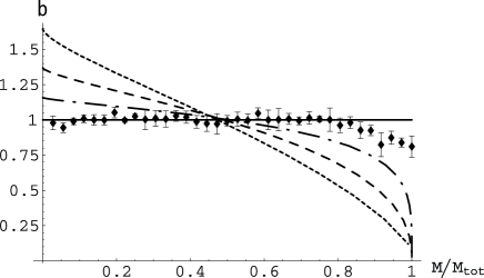
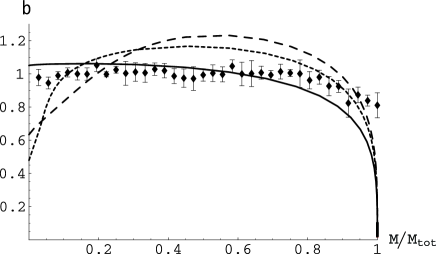
In Fig.8, we depicted the LV ratio $b$ as a function of $M_{r}$ for $n\leq 5$. The data plots of numerical situation are located almost everywhere on the constant line of $n=5$ Plummer’s model except for the outer region. As the value of $n$ decreases, the slope of function $b(M_{r})$ becomes steeper and deviates more from the LV relation (6).

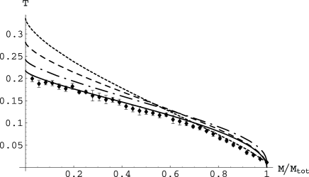
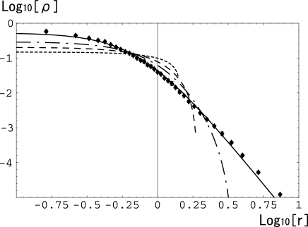
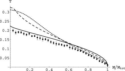
TM relation of Plummer’s model is obtained as (35) and the slope $dT/dM_{r}$ diverges as $M_{r}\rightarrow 0$. This discrepancy is plausible, since (9) is unphysical in the inner region. However the deviation from the linear TM relation is conspicuous only in the central part of the bound state,i.e., $M_{r}/M_{tot}<0.05$. This is consistent with the result that the unphysical region of (9) is at most inner five percent of the total mass. The slope of Plummer’s model becomes almost constant and the data plots are located almost everywhere in the middle region from $0.2M_{tot}<M_{r}<0.8M_{tot}$. In fact, the coincidence of the Plummer’s model to to the numerical data is remarkable, when we normalize both of the physical variables with the unit of $G=r_{h}=M_{tot}$, where $r_{h}$ is a half-mass radius of the bound system. (Fig.9 and Fig.10).

However, the polytropes with $n\sim 5$ fail in keeping the TM relation in the outer region since $T(M_{r})$ falls off steeply there (Fig.9). Recalling that the constant slope of TM relation up to the outer region is a key gradient for the DT distribution Osamu04 , the polytropes with $n\sim 5$ fail in reproducing the velocity distribution characteristic after a cold collapse. From (24) and (31), the mass density of Plummer’s solution behaves as $\propto r^{-5}$ in the outer region. This is also inconsistent with the numerical results and with the behavior of (9).

Secondly, we examined King models. King models have often been applied to fit the photometries of elliptical galaxies (e.g. Kormendy77 ; Bertin88 ). They are conventionally analyzed with the concentration parameter $c:=\log_{10}(r_{t}/r_{c})$, where $r_{t}$ and $r_{c}$ are the tidal radius and the core radius, respectively Binney87 . It is shown that the King model with $c\sim 2.25$ fits the observational $R^{1/4}$ law quite well Kormendy77 . Here we examined the LV relation and the TM relation for King models in the range $0.5<c<3.5$. For the family of such a parameter range, $b(M_{r})$ becomes smaller in the central part for larger value of $c$, which means that the potential energy is locally more dominated than the kinetic energy in the central part. By contrast, for $c\sim 0.5$, the virial ratio becomes flat close to the center and takes the similar form to those of polytropes with $n\sim 5$(Fig.11). As for the TM relation for King models, $T(M_{r})$ of the numerical result fits well to the case with $c\sim 0.5$ in the inner part $M<0.6M_{tot}$ but shifts to the case with $c\sim 2.7$ in the outer part (Fig.12). The density profiles of King models with $c>2.0$ also fit well to the numerical data in the outer part, where it behaves as $\rho\sim r^{-3}-r^{-4}$. This is consistent with the fact that the case with $c\sim 2.25$ fits to the observational $R^{1/4}$ law quite well. In contrast, the density profile for the case with $c\sim 0.5$ deviates from the numerical results remarkably.

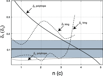
Finally, we estimate the deviations from LV relation and linear TM relation for polytropes and King models more quantitatively. Here we define the deviations from LV relation as $\delta_{v}:=\sqrt{\left\langle\langle(b-1)^{2}\right\rangle\rangle}$ where $\left\langle\langle\ast\right\rangle\rangle$ denote the average of the functions of $M_{r}$ defined as

$$\left\langle\langle\ast\right\rangle\rangle:=\frac{1}{{M_{tot}}}\int_{0}^{M_{tot}}{\;\ast\;dM_{r}}.$$ (16)

For the definition of the deviation from linear TM relation, we first linearly extrapolate the function $T_{e}(M_{r})$ as the form of $T_{e}(M_{r})=AM_{r}+B$. Then we define the deviation as

$$\delta_{t}:={\frac{\sqrt{\left\langle\langle(T-T_{e})^{2}\right\rangle\rangle}}{T_{1/2}}},$$ (17)

where $T_{1/2}$ is the local temperature at the half mass radius. In the parameter range we examined, we plotted both $\delta_{v}$ and $\delta_{t}$ for polytropes and King models (Fig.14). We also calculated the $\delta_{v}$s derived from the numerical simulations of cold collapse. They are obtained by averaging $(b(M_{r}/M_{tot})-1)^{2}$ at each $M_{r}$ in the same way as the integral (16). We got the result that the $\delta_{v}$ derived from the simulations in Fig.1 and Fig.3 takes the value $0.106\pm 0.053$, which is depicted as the gray zone in Fig.14. The parameter range whose $\delta_{v}$ exceeds this gray zone is considered to be incompatible with the numerical simulations in Fig.3.

It is obvious that the $\delta_{v}$ almost vanishes for the polytropes $n\sim 5$, since $n=5$ Plummer’s model exactly satisfies the LV relation, but for $n$ becomes small, $\delta_{v}$ becomes larger and exceeds the gray zone for $n\lesssim 3$ in Fig.14. Hence polytropes with $n\lesssim 3$ cannot follow the LV relation as well as the results of numerical simulations. On the other hand, the $\delta_{t}$s for polytropes are almost constant for any parameter range $0.5<n<5$ and the value is almost $0.05$. As for King models, the $\delta_{v}$ is larger than $0.1$ for all of the parameter range and has a peak around $c=2$. Especially, the $\delta_{v}$ of $1.6\gtrsim c\gtrsim 2.9$ is larger than $0.2$, which obviously exceeds the gray zone in Fig.14. This is in contrast to the fact that the surface brightness of King models fits well to $R^{1/4}$ law in this parameter range. On the other hand, the $\delta_{t}$s of King models are less than $0.1$ except for the high concentration case $c\gtrsim 3$. The strong deviation for $c\gtrsim 3$ is obvious, since the central temperature becomes much higher than those in the outer side for this parameter range.

In summary, we can see the remarkable difference between the polytrope sequence and the King sequence as the collisionless static system. In the case with King, the higher value of parameter $3.0>c>2.0$ is favorable to the density profile or linear TM relation but is not for the LV relation. The lower parameter range $0.5<c<1.0$ is favorable both to the linear TM relation and to the LV relation but is not for the density profile. Hence there is no parameter range in King model which is favorable to all of the characteristics of the bound state after a cold collapse. On the other hand, as for the polytrope, the parameter value $n\sim 5$ is favorable to all of those characteristics in the bound state after a collapse. Note that we can see the difference when we pay attention not only to the density profile but also to the velocity information such as the LV relation or linear TM relation.

Concerning the detail of the behaviour of physical quantities for $n\sim 5$ polytropes with the centrally flat boundary condition such as Plummer’s model, they fit quite well to the numerical results in the inner region, $M_{r}<0.6M_{tot}$. In the outer region, however, both the density profile and the TM relation deviate from the numerical data. We will comment on these failures of the Plummer’s model or $n\sim 5$ polytropes in the outer part from a viewpoint of the anisotropy of a velocity dispersion in the concluding remarks.

Figure 8: LV relation for polytropes with the unit of $G=r_{h}=M_{tot}=1$. The solid curve refers to the LV ratio $b(M_{r}/M_{tot})$ as a function of cumulative mass $M_{r}/M_{tot}$ for Plummer’s model. The other curves refer to $b(M_{r}/M_{tot})$ for polytropes with $n=3.0$ (dot-dashed), $n=1.5$ (dashed), $n=0.51$ (dotted). The plots represent the numerical data of SC ($\bar{b}_{t}=0,a=0$) with $N=10^{4}$.

Figure 9: Temperature versus cumulative Mass ($M_{r}$) for polytropes with the unit of $G=r_{h}=M_{tot}=1$. The solid curve refers to the local temperature $k_{B}T/m$ for Plummer’s model (35). The other curves refer to $k_{B}T/m$ for polytropes with $n=3.0$ (dot-dashed), $n=1.5$ (dashed), $n=0.51$ (dotted). The plots represent the numerical data of SC ($\bar{b}_{t}=0,a=0$) with $N=10^{4}$.

Figure 10: The density for polytropes (33) with the unit of $G=r_{h}=M_{tot}=1$. The solid curve refers to the density for Plummer’s model. The other curves refer to the density for polytropes with $n=3.0$ (dot-dashed), $n=1.5$ (dashed), $n=0.51$ (dotted). The plots represent the numerical data of SC ($\bar{b}_{t}=0,a=0$) with $N=10^{4}$.

Figure 11: The same as Fig.8 but for King models with the unit of $G=r_{h}=M_{tot}=1$. The solid curve refers to $b(M_{r}/M_{tot})$ for King model with $c=0.67$. The other curves refer to $b(M_{r}/M_{tot})$ for King models with $c=2.12$ (dashed), $c=2.72$ (dotted). The plots represent the numerical data of SC ($\bar{b}_{t}=0,a=0$) with $N=10^{4}$.

Figure 12: The same as Fig.9 but for King models with the unit of $G=r_{h}=M_{tot}=1$ . The solid curve refers to $k_{B}T/m$ for King model with $c=0.67$. The other curves refer to $k_{B}T/m$ for King models with $c=2.12$ (dashed), $c=2.72$ (dotted). The plots represent the numerical data of SC ($\bar{b}_{t}=0,a=0$) with $N=10^{4}$.

Figure 13: The same as Fig.10 but for King models with the unit of $G=r_{h}=M_{tot}=1$. The solid curve refers to the density for King model with $c=0.67$. The other curves refer to the density for King models with $c=2.12$ (dashed), $c=2.72$ (dotted). The plots represent the numerical data of SC ($\bar{b}_{t}=0,a=0$) with $N=10^{4}$.

Figure 14: Deviation $\delta_{v}$ and $\delta_{t}$ versus model parameters for polytropes and King models. Residuals with respect to polytrope index $n$ for polytropes and concentration parameter $c$ for King models are plotted. Each curve refers to $\delta_{v}$ for polytropes (solid), $\delta_{v}$ for King (dashed), $\delta_{t}$ for polytropes (dotted), $\delta_{t}$ for King (dot-dashed). The gray zone refers to the range of $\delta_{v}=0.106\pm 0.053$ derived from the numerical simulations of cold collapse in Fig.1 and Fig.3. Thick horizontal line denotes $\overline{\delta_{v}}=0.106$.

VII Concluding remarks

In this paper, we have proposed (a) the linear TM relation and (b) the LV relation as the hypotheses of self-gravitating structures after a cold collapse. Based on these two hypothetical proposals, we have uniquely determined the mass density profile (9) in the quasi-equilibrium state.

Our density profile behaves as $\rho\sim r^{-4}$ in the outer region and fits well both to the data of cold collapse simulations. Although this density profile is unphysical in the inner region, where it decreases with the decreasing radius, we showed that such an unphysical region is just a few percent around the central region of the bound state. Hence, we can safely neglect this region at least for the resolution of our numerical results.

In the central region, we also have to notice the relaxation process in such a central region. In fact, we examined how two-body relaxation is developed in a bound state after a cold collapse. We estimated the time scale of the two-body relaxation with $t^{\ast}_{rel}$, which is defined as the time when the region within a half-mass radius achieves a two-body relaxation on average. Both the linear TM relation and the LV relation appear even when the two-body relaxation is not attained. Hence, we can say that our two hypotheses are not affected through the two-body relaxation but are characteristic even in collisionless system in our estimation with $t^{\ast}_{rel}$.

From a viewpoint of these two hypotheses, we compared our results with two isotropic static models,i.e., polytropes and King models. The polytrope with $n=5$ is special among those models, since it exactly satisfies the LV relation. Plummer’s model, the polytrope with $n=5$ with a flat boundary condition at the center also satisfies the constant TM relation quite well in the intermediate region $0.2M_{tot}<M_{r}<0.8M_{tot}$. Moreover, its density fits well to the numerical data quite well in this intermediate region. On the other hand, both its TM relation and density profile in the outer region are slightly shifted from those in cold collapse simulations: the temperature falls off more steeply and the density behaves as $r^{-5}$ in the outer region. As for King models, in contrast, there is no parameter range in which both the TM relation and density profile fit well to the numerical data even in the intermediate region.

We also examined the deviations from the two hypotheses quantitatively for these two models. Only the polytropes with $n\sim 5$ are acceptable in that their deviations from both of the hypotheses are compatible with the numerical results of cold collapse. The LV relation imposes a strong constraint for these models. Especially for King models, the deviation from LV relation takes the maximum value around the parameter $c\sim 2$, in which the surface brightness fits well to $R^{1/4}$ law. This suggests that considering only the asymptotic behavior of the bound state is not enough to describe the collisionless static models to express observational or numerical results.

Combining the results for the above two models, we can speculate that Plummer’s model follows both of the hypotheses we proposed (a) LV relation and (b) linear TM relation. However, this model is lack of the following properties of the bound states in the actual simulations of cold collapse: (i) deviation from a hydrostatic equilibrium state and (ii) anisotropy of velocity dispersion in the outer region.

As for (i), the hydrostatic equilibrium condition is not attained especially when the violent degree of the initial collapse is strong, since the bound state slowly expands outward and is not balanced with a gravitational force after a cold collapse. Hence, to express these conditions we may have to consider not the static solution but the stationary solution admitting the coherent motion of matters.

As for (ii), we derived that for a mild collapsing case, the LV relation fluctuates more largely in the outer region and the slope of the TM relation at this region becomes a little steeper at least in the collisionless stage. We suspect that these results are related to the anisotropy of this system. Hence for more precise description of the system possessing two hypotheses, it seems necessary to treat the model with the anisotropy of the velocity dispersion. So far several collisionless static models with the anisotropic velocity dispersions or with the non-spherical symmetry have been proposed Henon73 ; Evans05 ; Bertin84 ; Stiavelli85 ; Dejonghe87 ; Gerhard91 ; Bertin03 . Incompleteness of the violent relaxation or the existence of conservative quantities during the phase mixing seem to be a candidate as the model to induce such anisotropy Lynden67 ; Stiavelli85 . The hypotheses we proposed are expected to be used as a guideline to build up the models following the characters of the bound states after a cold collapse by combining with these anisotropic models.

It also seems important how widely our two hypotheses are applicable in more general mixing processes including a merging process which yields a cuspy density profile in the central region Navarro96 . If we want to know the detail of such a tiny central region, such as the existence of the cuspy density profile, we have to treat such a central region more carefully. We speculate that in such a region, at least one of the two hypotheses we proposed will be broken. These points are now under investigation.

Appendix A Mass fraction of the centrally flat region against the outer analytical solution (9)

The analytical solution (9) has an inner unphysical region at $r<r_{\ast}$. Since the density goes to zero toward the center in this region, the cumulative mass in this region becomes very small. Here we will check how much the value is modified when we put the constant mass density in this region and connect it to the analytical solution at $r=r_{\ast}$. From the continuity at $r=r_{\ast}$, the density becomes

$$\rho=\left\{{\begin{array}[]{*{20}c}{\rho_{0}\left({{4\mathord{\left/{\vphantom{4e}}\right.\kern-1.2pt}e}}\right)^{4}\hfill}&{\left({r<r_{*}}\right)\hfill}\\ {\rho_{0}\left({{{r_{0}}\mathord{\left/{\vphantom{{r_{0}}r}}\right.\kern-1.2pt}r}}\right)^{4}e^{-{{r_{0}}\mathord{\left/{\vphantom{{r_{0}}r}}\right.\kern-1.2pt}r}}\hfill}&{\left({r\geq r_{*}}\right)\hfill}\\ \end{array}}\right..$$ (18)

The cumulative mass at $r=r_{\ast}$ is

$$M_{in}=4\pi\rho_{0}r_{0}^{3}\left({\frac{4}{{3e^{2}}}}\right).$$ (19)

The cumulative mass outside $r_{\ast}$ is

$$M_{out}=4\pi\int_{{{r_{0}}\mathord{\left/{\vphantom{{r_{0}}4}}\right.\kern-1.2pt}4}}^{\infty}{\rho_{0}\left({\frac{{r_{{}_{0}}}}{r}}\right)^{4}e^{-{{r_{0}}\mathord{\left/{\vphantom{{r_{0}}r}}\right.\kern-1.2pt}r}}}r^{2}dr=4\pi\rho_{0}r_{0}^{3}\left({1-e^{-4}}\right).$$ (20)

Hence the mass fraction of the inner region becomes

$$\frac{{M_{in}}}{{M_{tot}}}=\frac{{M_{in}}}{{M_{in}+M_{out}}}=\frac{4}{{3e^{4}+1}}\approx 0.0243.$$ (21)

Appendix B Derivation of the LV relation for polytropes

Following Binney87 , we use the notation using the relative energy $\epsilon$ and relative potential $\phi$ defined as

$$\tilde{E} := -E+\Phi_{\ast},$$

$$\phi := -\Phi+\Phi_{\ast},$$ (22)

respectively. For polytropes, using these notations, the distribution function is described as

$$f(\tilde{E})=\left\{{\begin{array}[]{*{20}l}\kappa_{1}\tilde{E}^{n-3/2},&\;(\tilde{E}\geq 0);\\ 0,&\;(\tilde{E}<0),\\ \end{array}}\right.$$ (23)

For (23), density $\rho$ and temperature $T$ are simply expressed as

$$\rho=c_{n}\phi^{n},$$ (24)

$$<v^{2}>={\frac{3k_{B}T}{m}}={\frac{3}{n+1}}\phi,$$ (25)

where $c_{n}:=(2\pi)^{3/2}{\frac{(n-3/2)!}{n!}}\kappa_{1}$.

From (3) and (22), we get

$$\overline{W}_{r}={\frac{M_{r}\Phi_{\ast}}{2}}-2\pi\int_{0}^{R}\phi\rho(r)r^{2}dr.$$ (26)

From (4),(26), and (25), we get

$$\overline{K}_{r}+{\frac{3}{n+1}}\overline{W}_{r}={\frac{3}{2(n+1)}}M_{r}\Phi_{\ast}.$$ (27)

Especially for $n=5$, from the condition $\Phi_{\ast}=0$, the LV relation $2\overline{K}_{r}/|\overline{W}_{r}|=1$ is obtained.

Appendix C Derivation of TM relation for Plummer’s model

Following Binney87 , we define the dimensionless variables

$$\psi:=\phi/\phi_{0}\;\;\;\;s:=r/b,$$ (28)

where $\phi_{0}$ is the value of the relative potential at the center and $b:=\{4\pi Gc_{n}\phi_{0}^{n-1}\}^{-1/2}$. Then, $\psi$ is followed by Lane-Emden equation,

$${\frac{1}{s^{2}}}{\frac{d}{ds}}\left(s^{2}{\frac{d\psi}{ds}}\right)=\left\{{\begin{array}[]{*{20}l}-\psi^{n},&\;(\psi\geq 0);\\ 0,&\;(\psi\leq 0),\\ \end{array}}\right.$$ (29)

with the boundary condition

$$\lim_{s\rightarrow\infty}\psi(s)=\psi_{\ast},$$ (30)

where $\psi_{\ast}:=\Phi_{\ast}/\phi_{0}$. Especially for $n=5$, the solution of (29) with the flat boundary condition at the center becomes

$$\psi={\frac{1}{\sqrt{1+s^{2}/3}}},$$ (31)

and meets the boundary condition

$$\lim_{s\rightarrow\infty}\psi(s)=\psi_{\ast}=0.$$ (32)

The density is described as

$$\rho=\psi^{n}=\frac{1}{(1+s^{2}/3)^{n/2}}.$$ (33)

In spherically symmetric case, the cumulative mass $M_{r}$ is expressed as $M_{r}={\frac{r^{2}}{G}}{\frac{d\Phi}{dr}}$, whose dimensionless form becomes

$$M_{r}=-s^{2}{\frac{d\psi}{ds}},$$ (34)

and the total mass $M_{tot}$ is equal to $\sqrt{3}$. Substituting (31) into dimensionless form of (25) and (34) and eliminating $s$, we can easily derive the TM relation of Plummer’s model as

$${\frac{k_{B}T}{m}}={\frac{1}{6}}\sqrt{1-\left({\frac{M_{r}}{M_{tot}}}\right)^{2/3}}.$$ (35)

References

- (1) Lynden-Bell D.,1967, MNRAS, 136, 101
- (2) Hénon M.,1964,Ann.Astrophys. 27,83
- (3) Van Albada T.S.,1982, MNRAS, 201, 939
- (4) Merrall T.E.C. and Henriksen R.N., 2003 , ApJ,595, 43
- (5) Dejonghe H., 1987 , MNRAS, 224, 13
- (6) Gerhard O. E., 1993 , MNRAS, 265, 213
- (7) Binney J.J. and Mamon G.A., 1982 , MNRAS,200, 361
- (8) Nakamichi A. and Morikawa M., 2004, Physica A, 341, 215
- (9) Kazantzidis S., Magorrian J. and Moore B., 2004, ApJ, 601, 37
- (10) Kawai A., Fukushige T., Makino J. and Taiji M., 2000, PASJ 52, 659
- (11) Iguchi O., Sota Y., Tatekawa T., Nakamichi A. and Morikawa M., 2005, Phys. Rev. E, 71, 016102
- (12) Eddington A.S.,1916, MNRAS,76,572.
- (13) Evans N. W. and An J., 2005, MNRAS, 360 492.
- (14) Jaffe W.,1987, Structure and Dynamics of Elliptical Galaxies, I.A.U.Symp. 127, 511
- (15) Makino J., Akiyama K., and Sugimoto D.,1990, PASJ 42, 205
- (16) Spitzer L. Jr., Dynamical Evolution of Globular Clusters (Princeton: Princeton Univ. Press)
- (17) Binney J. J. and Tremaine S., Glactic Dynamics(Princeton University Press, Princeton, 1987).
- (18) BertinG., Saglia R. .P. and Stiavelli M., 1988, ApJ, 330, 78
- (19) Kormendy J.,1977, ApJ 218, 333
- (20) Hénon M.,1973,A&A 24,229
- (21) Bertin G. and Stiavelli M., 1984, A&A, 137, 26
- (22) Stiavelli M. and Bertin G., 1985, MNRAS, 217, 735
- (23) Gerhard O. E., 1991 , MNRAS, 250, 812
- (24) Bertin G. and Trenti M., 2003, ApJ, 584, 729
- (25) Navarro J. F., Frenck C. S. and White S. D. M., 1996, ApJ. 462, 563