Skewness as a test for Quartessence
Abstract
Quartessence is one of the alternatives to -CDM that has lately attracted considerable interest. According to this unifying dark matter/energy scenario, the Universe evolved from an early non-relativistic matter-dominated phase to a more recent accelerated expansion phase, driven by a single fluid component. Recently, it has been shown that some problems of the quartessence model, such as the existence of instabilities and oscillations in the matter power spectrum, can be avoided if a specific type of intrinsic entropy perturbation is considered. In the present article we explore the role of skewness in constraining this non-adiabatic scenario. We show that non-adiabatic quartessence and quintessence have different signatures for the skewness of the density distribution on large scales and suggest that this quantity might prove helpful to break possible degeneracies between them.
I Introduction
According to the current standard cosmological model, the dynamics of the universe would be dominated by two unknown components: dark-matter (DM), responsible for structure formation, and dark-energy (DE), that causes the accelerated expansion. Although there are several candidates for both DM and DE, there is still no evidence of either of them in laboratory physics. From the point of view of simplicity, it would be interesting to explore the possibility that a single component plays the role of both DE and DM, reducing from two to one the unknown constituents of the universe. A model that provides a single description of DE and DM through “unifying-dark-matter” or simply quartessence makler03 has attracted a lot of interest recently. A prototype of this model is given by the quartessence Chaplygin model (QCM) kamenshchik01 .
Both the background and linear fluctuations were extensively studied for QCM, and were compared to observational data. The generalized Chaplygin gas (as quartessence) appears to be compatible with all available data regarding the expansion history (see e.g. ref. makler03b and refs. therein). For adiabatic perturbations, a linear analysis was done for the CMB amendola03 and LSS beca03 . In this case, only QCM models close to the “CDM limit” are allowed. Recently, it was shown that problems (pointed out in sandvik02 ), such as the existence of instabilities and oscillations in the matter power spectrum of QCM, can be avoided if a specific type of intrinsic entropy perturbation is considered. Such non-adiabatic model is consistent with the 2dF power spectrum for any value of the model parameters in the permitted interval, as long as the effective shape parameter assumes certain values reis03b . An “averaging problem” was also pointed out as a shortcoming of quartessence avelino03 . However, it is straightforward to show that the above mentioned non-adiabatic quartessence does not suffer this kind of problem obs .
Thus, up to the present time, we can say that adiabatic quartessence is disfavored by the data, but it is not possible to distinguish non-adiabatic quartessence from concordance models like CDM and quintessence using the previously considered observables. However, as we shall see, measurable differences in the predictions of these models appear clearly in the nonlinear regime, in particular in the skewness of the matter distribution in large scales. In our investigation we specifically consider three different quartessence models. All of them have the CDM model as a limiting case for the background solution. The analysis of these three cases indicates that our result should be applicable to more generic quartessence models.
While most studies of the nonlinear regime deal with the clumping of pressureless fluid (DM), in the case of quartessence it is imperative that one includes the effects of pressure. Accordingly, we apply, and somewhat extend to include relativistic pressure, a method for the computation of density cumulants developed in refs. bernardeau92 ; bernardeau94 ; fosalba98 .
II Gravitational growth for quartessence in the spherical collapse approximation
In our approach we consider the following newtonian-like equations lima ; reis03
| (1) |
| (2) |
| (3) |
Equations (1), (2) and (3) are, respectively, the Poisson, Euler and energy conservation equations, where relativistic effects of pressure (inertia and active gravitational mass) have been included. In these equations , , and stand for, the energy density, pressure, velocity field, and gravitational potential of the cosmic fluid, and we take . In the linear regime, for (see bellow), system (1-3) gives exactly the same equations as the relativistic perturbation theory in a particular gauge reis03 . Also the (nonlinear) energy conservation and the Raychadhuri equations derived from this system are formally identical to the general relativistic ones ellis in this case, which provides a motivation for the above system.
It is useful to split the dynamical variables into their background and inhomogeneus parts, i.e. we write: , , , and . Here is the Hubble parameter, stands for the scale factor, and the overbar “” denotes background (average) quantities. Introducing comoving coordinates , neglecting shear and vorticity, and taking into account the background equations (assuming critical density), we obtain, after some algebra, the following differential equation for the density contrast ,
| (4) |
In the above equation the prime symbol denotes differentiation with respect to , , and hu . In the linear approximation, in the special case in which perturbations are adiabatic we have . However, as discussed in sandvik02 , in this case, the right hand side of (4) gives rise to oscillations and instabilities in the mass power spectrum that render the model unacceptable. This problem can be circumvented if non-adiabatic perturbations such that , are considered reis03b . In the following we assume this is the case such that Eq. (4) simplifies to,
| (5) |
To study the weakly nonlinear regime of structure formation and compute the higher order moments of the density distribution, it is useful to expand as bernardeau92 ; bernardeau94 ; fosalba98 ,
| (6) |
where is a small perturbation. Using the above expansion we obtain for the linear () and second order () factors the following differential equations,
| (7) |
and
| (8) |
Analogously, higher order modes can be obtained recursively by using the solutions of the differential equations for the lower order terms. Of special interest is the second-order equation. If we start with Gaussian initial conditions, it is associated with the emergence of non-Gaussian features in the matter density field. Further, can be related to the skewness of the cosmic field peebles ; fry . In this case, the unsmoothed skewness is given by .

We now consider the following quartessence models:
| (9) | |||||
| (10) | |||||
| (11) |
When , all the models above have CDM as a limiting case for the background. At first and higher order in perturbation theory, however, these quartessence models with , have distinct behavior as compared to that of dark-matter in CDM.
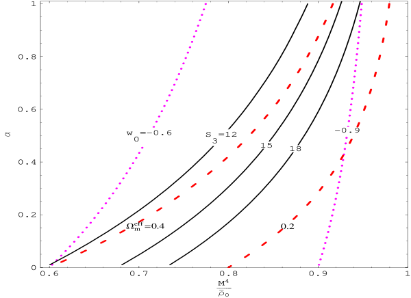
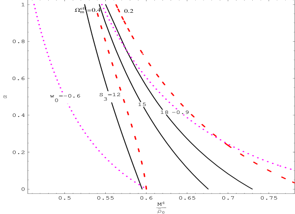
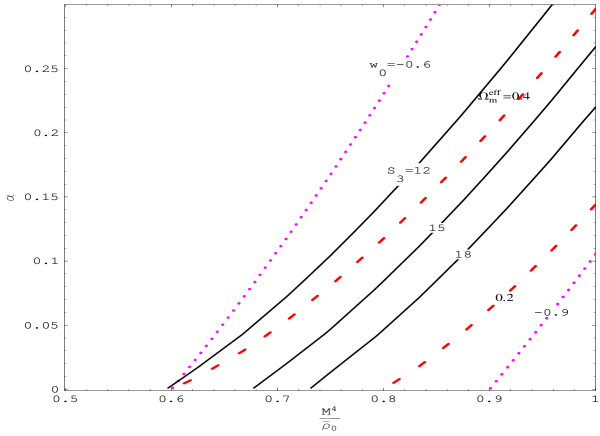
In Figs. , and we show contours of constant skewness values at present time for the above models. In our numerical computation, we consider that at , the growing modes and assume the Einstein-de Sitter behavior: , , and such that at that time. We also include in the figures two curves with constant effective matter density parameter ( and ). Here, , where is the present value of the background energy density. We should expect the region between these two curves to be, roughly, the one allowed by current observational data. For instance, in makler03b it was shown that, for QCM, constraints from cluster x-ray data (that are the most restrictive ones), essentially correspond to these curves. The same holds for the other quartessence models. From the figures it is clear that, for all the considered models, the skewness in these regions assumes values between . This strongly contrasts with what is expected in CDM and quintessence, where one obtains , weakly sensitive to the cosmological parameters bernardeau94 ; gaztanaga01 ; benabed01 ; multamaki03 ; multamaki03b .
At first sight this difference could be interpreted as an indication that quartessence models are inconsistent with large-scale skewness measurements skewobs . However, care should be taken when analyzing this issue. Whereas in the discussion above baryons were neglected, measurements of skewness from large-scale galaxy distribution, are based on counting luminous objects, not the dark component. Eqs. (1)-(5) can be easily generalized to include baryons makler04 . The main outcome is that the quartessence skewness is not substantially affected by the presence of a small amount () of baryons, but on the other hand, the baryonic skewness () is nearly constant with redshift, i.e. . Therefore, again baryons behave differently from the dark component as in the adiabatic quartessence power-spectrum case beca03 . We remark that this holds even for .
Further investigation is necessary to clarify to what extent do skewness measurements from galaxy distribution constrain quartessence models. Although more challenging to observe, a potentially powerful probe is the lensing (convergence) skewness bernardeau02 , that is sensitive to both baryons and quartessence. According to skewlens current lensing observations are still too noisy to allow strong constraints on cosmological parameters. On the other hand, as discussed above, quartessence predictions for the skewness are quite different from CDM models and its variants. Thus, we expect that present and upcoming data might discriminate among these two classes of models.
In the present work, we have not quantitatively compared quartessence predictions with observations. Our goal here is more modest; we essentially use Figs. , and to stress out the important fact that non-adiabatic quartessence and concordance models like CDM and quintessence could be observationally distinguished by skewness measurements. We leave this investigation for a future work makler04 . Finally, we remark that our results do not apply straightforwardly to quartessence models with a scalar field with, for instance, a non-canonical kinetic term scherrer , but these models have yet to be tested against background and power spectrum data.


Acknowledgements.
The authors would like to thank the Brazilian research agencies CAPES, CNPq and FAPERJ for financial support.References
- (1) M. Makler, S.Q. Oliveira, and I. Waga, Phys. Lett. B 555, 1 (2003).
- (2) A. Kamenshchik, U. Moschella, and V. Pasquier, Phys. Lett. B 511, 265 (2001); M. Makler, Gravitational Dynamics of Structure Formation in the Universe, PhD Thesis, Brazilian Center for Research in Physics (2001); N. Bilić, G.B. Tupper, and R.D. Viollier, Phys. Lett. B 535, 17 (2002); M.C. Bento, O. Bertolami, and A.A. Sen, Phys. Rev. D 66, 043507 (2002).
- (3) M. Makler, S.Q. Oliveira, and I. Waga, Phys. Rev. D 68, 123521 (2003).
- (4) L. Amendola, F. Finelli, C. Burigana, and D. Carturan, JCAP 07, 005 (2003). See also D. Carturan, F. Finelli, Phys.Rev. D 68, 103501 (2003) and R. Bean and O. Dore, Phys.Rev. D 68, 023515 (2003) for the case of the Chaplygin fluid as only dark energy.
- (5) L.M.G. Beça, P.P. Avelino, J.P.M. de Carvalho, and C.J.A.P. Martins, Phys. Rev. D 67, 101301(R) (2003).
- (6) H. Sandvik, M. Tegmark, M. Zaldarriaga, and I. Waga, astro-ph/0212114 (v2), to appear Phys. Rev. D (2004).
- (7) R.R.R. Reis, I. Waga, M.O. Calvão, and S.E. Jorás, Phys. Rev. D 68, 061302(R) (2003).
- (8) P.P. Avelino, L.M.G. Beça, J.P.M. de Carvalho, C.J.A.P. Martins, and E.J. Copeland, Phys. Rev. D 69, 041301(R) (2004).
- (9) Since , for non-adiabatic quartessence models we always have .
- (10) F. Bernardeau, Astrophys. J. 392, 1 (1992).
- (11) F. Bernardeau, Astrophys. J. 433, 1 (1994).
- (12) P. Fosalba and E. Gaztañaga, Mon. Not. R. Astron. Soc. 301, 503 (1998).
- (13) J.A.S. Lima, V. Zanchin, and R. Brandemberger, Mon. Not. R. Astron. Soc. 291, L1 (1997).
- (14) R.R.R. Reis, Phys. Rev. D 67, 087301 (2003), Erratum-ibid. D 68, 089901 (2003).
- (15) G.F.R. Ellis, Relativistic Cosmology. In R. K. Sachs, editor, General Relativity and Cosmology, proceedings of the XLVII Enrico Fermi Summer School, Academic Press, 1971.
- (16) W. Hu, Astrophys.J. 506, 485 (1998).
- (17) P.J.E. Peebles, The Large Structure of the Universe, Princeton University Press, Princeton, (1980).
- (18) J. Fry, Astrophys.J. 279, 499 (1984).
- (19) E. Gaztañaga and J.A. Lobo, Astrophys. J. 548, 47 (2001).
- (20) K. Benabed and F. Bernardeau, Phys. Rev. D 64, 083501 (2001).
- (21) T. Multamäki, E. Gaztañaga, and M. Manera, Mon. Not. R. Astron. Soc. 344, 761 (2003).
- (22) T. Multamäki, M. Manera, and E. Gaztañaga, Phys. Rev. D 69, 023004 (2004).
- (23) M. Makler et al., in preparation (2004).
- (24) E. Gaztañaga and J.A. Frieman, Astrophys. J. 437, L13 (1994); F. Hoyle, I. Szapudi, and C.M. Baugh, Mon. Not. R. Astron. Soc. 317, L51 (2000); I. Szapudi, M. Postman, T.R. Lauer, and W. Oegerle, Astrophys. J. 548, 114 (2001); I. Szapudi et. al., Astrophys. J. 570, 75 (2002); for review see F. Bernardeau, S. Colombi, E. Gaztañaga, and R. Scoccimarro, Phys. Rep. 367, 1 (2002).
- (25) F. Bernardeau, L. van Waerbeke , and Y. Mellier, Astron. Astrophys. 322, 1 (1997).
- (26) F. Bernardeau, Y. Mellier, and L. van Waerbeke, Astron. Astrophys. 389, L28 (2002); U.-L. Pen et al., Astrophys. J. 592, 664 (2003).
- (27) R. J. Scherrer, astro-ph/0402316 (v2).